Hot gas flows on global and nuclear galactic scales

Abstract

Since its discovery as an X-ray source with the $Einstein$ Observatory, the hot X-ray emitting interstellar medium of early-type galaxies has been studied intensively, taking advantage of observations of improving quality performed by the subsequent X-ray satellites $ROSAT$, $ASCA$, $Chandra$ and $XMM-Newton$, and comparing the observational results with extensive modeling by means of numerical simulations. The hot medium originates from the ejecta produced by the normal stellar evolution, and during the galaxy lifetime it can be accumulated or expelled from the galaxy potential well. The main features of the hot gas evolution are outlined here, focussing on the mass and energy input rates, the relationship between the hot gas flow and the main properties characterizing its host galaxy, the flow behavior on the nuclear and global galactic scales, and the sensitivity of the flow to major galaxy properties as the shape of the mass distribution and the mean rotation velocity of the stars.

1 Introduction

X-ray observations performed during the late 1970’s first revealed that early-type galaxies (ETGs) emit soft thermal X-rays and then host an interstellar medium (ISM), of a mass up to $\sim 10^{10}\,M_{\odot}$, that had not been discovered previously at other frequencies because of its high temperature ($T\sim 10^{7}$ K; see Fabbiano, this volume). Such a medium was the long sought phase fed by stellar mass losses and predicted by the stellar evolution studies (e.g., (FG, ; Mat89, )); in fact, both isolated ETGs and those in groups or clusters emit soft thermal X-rays Fab89 , which provides simple evidence that the hot ISM is mostly indigenous rather than accreted intergalactic medium. Besides solving a puzzle, this discovery opened the study of an important component of ETGs: it is a major ingredient of galactic evolution, see for example its role in feeding a central supermassive black hole and maintaining an activity cycle and starformation (e.g., (FC88, ; For05, ; Kor, ), and Ciotti & Ostriker, this volume), or that in polluting the space surrounding ETGs with metals, via galactic outflows (R93 , and Pipino, this volume), or finally in responding to environmental effects, as interaction with neighbors, stripping, sloshing, and conduction (e.g., (Acr, ; Sun07, ; K08, ), and Sarazin, this volume).

The most striking X-ray observational feature of ETGs is the wide variation in their luminosity ($L_{\rm X}$) values, of ${\mathrel{\mathchoice{\lower 2.9pt\vbox{\halign{$\m@th\displaystyle\hfil#\hfil$\cr>\crcr\sim\crcr}}}{\lower 2.9pt\vbox{\halign{$\m@th\textstyle\hfil#\hfil$\cr>\crcr\sim\crcr}}}{\lower 2.9pt\vbox{\halign{$\m@th\scriptstyle\hfil#\hfil$\cr>\crcr\sim\crcr}}}{\lower 2.9pt\vbox{\halign{$\m@th\scriptscriptstyle\hfil#\hfil$\cr>\crcr\sim\crcr}}}}}2$ orders of magnitude at any fixed galactic optical luminosity $L_{B}$, when $L_{B}>3\times 10^{10}L_{B,\odot}$ (Fab89, ; OS, ; Mem, ; Kim10, ). This feature cannot be explained by distance uncertainties, since a variation of the same size is present even in the distance-independent diagram of $L_{\rm X}/L_{\rm B}$ versus the central stellar velocity dispersion $\sigma_{c}$ (e.g., Esk, ). A number of reasons have been proposed as responsible for this large variation, of environmental nature (see Sarazin, this volume) or linked to the possibility for the gas content to evolve substantially during the ETG lifetime. In this latter context, many studies investigated with numerical simulations the dynamical evolution of the hot ISM in ETGs (SW, ; LM, ; Da90, ; Da91, ; C91, ; PC98, ; T09, ). In more recent times, the effect of feedback from a central supermassive black hole (MBH) has revealed as another potential contributor to the variation of the hot ISM luminosity (see Statler, and Ciotti & Ostriker, this volume).

Below I briefly review our current knowledge about the feeding and the energetics of the hot gas flows, concentrating on their dynamical state as a function of galactic mass and other major galaxy properties. Section 2 gives an updated summary of the fundamental elements entering the problem, the mass and energy inputs to the flow; Sect. 3 presents the general case for the evolution of the flow, pointing out the different behavior on the global and nuclear galactic scales, and making also use of a representative ETG; the effect of a central MBH, acting as a gravitating point mass, and the expectations for accretion feedback, are presented in Sect. 4; finally, Sect. 5 discusses the observed sensitivity of the flow to major galaxy properties as the flattening of the mass distribution, the mean rotational velocity of the stars, and the shape of the stellar profile.

2 Feeding and Energetics of the Hot Gas Flows

In this Section the fundamental processes and quantities at the basis of the origin and evolution of hot gas flows are introduced: their feeding via stellar mass losses (Sect. 2.1), their heating via type Ia supernovae explosions (Sect. 2.2), and their energy budget (Sect. 2.3).

2.1 The Stellar Mass Loss Rate

In ETGs the gas is lost by evolved stars mainly during the red giant, asymptotic giant branch, and planetary nebula phases. These losses originate ejecta that initially have the velocity of the parent star, then interact with the mass lost from other stars or with the hot ISM, and mix with it. The details of the interaction are controlled by several parameters, like the velocity of the mass loss relative to the hot phase, or the density of the ambient ISM Mat90 . Parriott & Bregman (PB and BP ), modeling the interaction with two-dimensional hydrodynamical simulations, found that most of the continuous mass loss from giant stars is heated to approximately the temperature of the hot ISM within few parsecs of the star; in the case of mass ejected by planetary nebulae, about half of the ejecta separates and becomes hot, and the other half creates a narrow wake that remains mostly cool, unless turbulent mixing allows for its heating on larger scales. Far infrared observations allow us to measure directly the stellar mass loss rate for the whole galaxy ($\dot{M}_{*}$); this was for example derived for nine local ETGs from $ISO$ data At . When rescaled by the luminosities of the respective galaxies, the values of $\dot{M}_{*}$ were found to vary by a factor of $\sim 10$, which was attributed to different ages and metallicities. The average of the observed rates was $\dot{M}_{*}=7.8\times 10^{-12}\,\,L_{B}(L_{B,\odot})$ M_⊙yr^-1, and was found to be in reasonable agreement with previous theoretical predictions At .

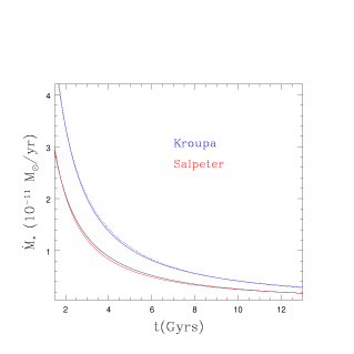
Figure 1: Evolution of the stellar mass loss rate $\dot{M}_{*}(t)$ according to the models in Mar05 , for a Salpeter IMF (solid line with best fit of Eq. 1 in red) and for a Kroupa IMF (dotted line with best fit of Eq. 1 in blue). Solar abundance is assumed, and a total stellar mass of 1 $M_{\odot}$ at an age of 12 Gyrs.

According to single burst stellar population synthesis models, most of the stellar mass is lost at early times, before an age of $\sim 2$ Gyr. For example, the mass lost by stars at an age of 2 Gyr is 25% of the total initial mass, for the Salpeter initial mass function (IMF), and 36% for the Kroupa IMF; at an age of 12 Gyr, the additional loss is of $\sim 4$% and 6% of the initial mass, for the same two IMFs respectively Mar05 . Figure 1 shows the trend of $\dot{M}_{*}(t)$ with time, estimated from the models in Mar05 for solar metal abundance. At an age of ${\mathrel{\mathchoice{\lower 2.9pt\vbox{\halign{$\m@th\displaystyle\hfil#\hfil$\cr>\crcr\sim\crcr}}}{\lower 2.9pt\vbox{\halign{$\m@th\textstyle\hfil#\hfil$\cr>\crcr\sim\crcr}}}{\lower 2.9pt\vbox{\halign{$\m@th\scriptstyle\hfil#\hfil$\cr>\crcr\sim\crcr}}}{\lower 2.9pt\vbox{\halign{$\m@th\scriptscriptstyle\hfil#\hfil$\cr>\crcr\sim\crcr}}}}}2$ Gyr, this trend can be approximated as:

$$\dot{M}_{*}(t)=10^{-12}\,A\,\times M_{*}(M_{\odot})\,\,t_{12}^{-1.3}\quad\quad\quad({\rm M_{\odot}yr^{-1}}),$$ (1)

where $M_{*}$ is the galactic stellar mass at an age of 12 Gyr, $t_{12}$ is the age in units of 12 Gyrs, and $A=2.0$ or 3.3 for a Salpeter or Kroupa IMF (see Fig. 1).

The relation above agrees well with previous theoretical estimates Mat89 ; C91 . Taking the stellar mass-to-light ratio in the B-band at an age of 12 Gyr ($M_{*}/L_{B}=9.17$ and 5.81, respectively for the Salpeter and Kroupa IMFs, Mar05 ), Eq. 1 gives $\dot{M}_{*}$(12 Gyr)= B $\times 10^{-11}\,L_{B}(L_{B,\odot})$ M_⊙yr^-1, with B=1.8 or B=1.9 for the Salpeter or Kroupa IMF. The latter relation gives a rate that is roughly double as large as the average of the observational estimates quoted above (At ), that however has a large variation around it, partly explained by differences in the ages and metallicities of the observed ETGs.

2.2 The Type Ia Supernovae Mass and Energy Input

The total mass loss rate of a stellar population $\dot{M}$ is given by the sum $\dot{M}(t)=\dot{M}_{*}(t)+\dot{M}_{\rm SN}(t)$, where one adds to $\dot{M}_{*}(t)$ (discussed in the previous Sect. 2.1) the rate $\dot{M}_{\rm SN}(t)$ of mass lost by type Ia supernovae (SNIa) events, the only ones observed in an old stellar population (e.g., Capp, ). The mass input due to SNIa’s is $\dot{M}_{\rm SN}(t)=1.4$ M${}_{\odot}\,R_{\rm SN}(t)$ M_⊙ yr^-1, where $R_{\rm SN}(t)$ (in yr^-1) describes the evolution of the explosion rate with time, since each SNIa ejects 1.4 M_⊙. In a detailed scenario for the SNIa precursors and their subsequent explosion past a burst of star formation (Gre05, ; Gre10, ), $R_{\rm SN}(t)$ experiences a raising epoch during the first 0.5-1 Gyr, at the end of which it reaches a peak, and then decreases slowly with a timescale of the order of 10 Gyr, and accounts for the present day observed rate. A parameterization of the rate after the peak, in number of events per year, is

$$R_{\rm SN}(t)=0.16(H_{0}/70)^{2}\times 10^{-12}\,\,L_{B}(L_{B,\odot})\,\,\,t_{12}^{-s}\quad\quad({\rm yr}^{-1}),$$ (2)

where $H_{0}$ is the Hubble constant in units of km s^-1 Mpc^-1, $L_{B}$ is the present epoch galaxy luminosity, and $s$ describes the past evolution; when $t_{12}=1$, Eq. 2 gives the rate for local ETGs in Capp , that has an uncertainty of $\pm 30$%. Recently, new measurements of the observed rates of supernovae in the local Universe, determined from the Lick Observatory Supernova Search (LOSS; Li ), gave a SNIa’s rate in ETGs consistent with that in Capp . For the rate in Eq. 2, and for $H_{0}=70$ km s^-1 Mpc^-1, one obtains $\dot{M}_{\rm SN}$(12 Gyr) =2.2$\times 10^{-13}L_{B}(L_{B,\odot})$ M_⊙ yr^-1, that is almost $\sim 100$ times smaller than the ”normal” stellar mass loss rate $\dot{M}_{*}$ (12 Gyr)$\approx 2\times 10^{-11}\,L_{B}(L_{B,\odot})$ M_⊙ yr^-1 derived above (Sect. 2.1).

SNIa’s provide also heating (Sect. 2.3 below) at a rate $L_{\rm SN}(t)$ that is the product of the kinetic energy injected by one event ($E_{\rm SN}\approx 10^{51}$ erg) times the rate $R_{\rm SN}(t)$. This assumes that the total of $E_{\rm SN}$ is turned into heat of the hot ISM, an assumption that is clearly an overestimate, but not totally unreasonable for the hot diluted gas (Mat89 ). Then

$$L_{\rm SN}(t)=E_{\rm SN}\times R_{\rm SN}(t)=5.1(H_{0}/70)^{2}\times 10^{30}\,L_{B}(L_{B,\odot})\,\,t_{12}^{-s}\quad\quad({\rm erg\,\,s}^{-1}),$$ (3)

and is plotted in Fig. 2 for $t_{12}=1$ and $H_{0}=70$ km s^-1 Mpc^-1. The SNIa’s specific heating, given by the total SNIa’s heating per total injected mass (approximated hereafter with $\dot{M}_{*}$) is

$${L_{\rm SN}\over{\dot{M}_{*}}}=1.6(H_{0}/70)^{2}\times 10^{50}\,{L_{B}(L_{B,\odot})\over A\,M_{*}(M_{\odot})}\,t_{12}^{1.3-s}\,\,\,\,\,({\rm erg\,\,M_{\odot}^{-1}})$$ (4)

where $\dot{M}_{*}$ given in Eq. 1 has been used. At an age $t_{12}=1$, for $H_{0}=70$ km s^-1 Mpc^-1, and using $\dot{M}_{*}$(12 Gyr) $\approx 2\times 10^{-11}\,L_{B}(L_{B,\odot})$ M_⊙ yr^-1 (valid for both IMFs, see below Eq. 1), one gets $L_{\rm SN}/{\dot{M}_{*}}\approx 8\times 10^{48}\,\,{\rm erg\,\,M_{\odot}^{-1}}$, that is a significant heating (with respect to, e.g., the specific binding energy of the gas, see Sect. 2.3 and Fig. 2).

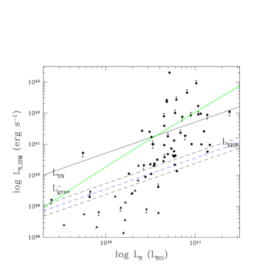
Figure 2: The X-ray luminosity of the hot ISM $L_{X,ISM}$ from $Chandra$ observations, versus the galactic $L_{B}$ (from corrected apparent magnitudes from Hyperleda, and distances from T01 ; DS1 , for $H_{0}=70$ km s^-1 Mpc^-1). $L_{X,ISM}$ is from DS1 (circles), D06 (triangles), NM (squares); downward (upward) arrows indicate upper (lower) limits. The dashed lines show the mean total luminosity from X-ray binaries derived from $Chandra$ data (in blue), and its $\pm 1\sigma$ uncertainty, from Kim10 . All X-ray luminosities have been recalculated for the 0.3–5 keV band, assuming the spectral shape in the original references. The solid line is $L_{SN}$ (Eq. 3); the green line is $L_{grav}^{-}$ (Eq. 7), calculated for $\dot{M}_{*}(12$ Gyrs) of the Kroupa IMF (Sect. 2.1), and representative galactic mass models (see also Sect. 3) with: a stellar de Vaucouleurs profile, $\sigma_{c}$ from the Faber-Jackson relation, an effective radius $R_{e}$ from the Fundamental Plane relation (Ber ), a NFW dark mass profile with a dark-to-luminous mass ratio of 5 in total (kom ), and of 0.6 within $R_{e}$ ((Cap06, ; Wei09, ; Shen, )), a ratio of the scale radii of the dark and stellar mass distributions of $r_{h}/R_{e}=1.5$.

During the galaxy lifetime, $L_{\rm SN}/{\dot{M}_{*}}\propto t^{1.3-s}$, and then can increase or decrease with time increasing, with consequences on the secular gas flow behavior ((LM, ; Da90, ; C91, ); Sect. 3). Early hydrodynamical simulations of hot gas flows enlighted the importance of the cosmological evolution of the SNIa’s rate to avoid excessive, and unobserved, mass accumulation at the galactic centers: if $L_{SN}$ decreases faster than $\dot{M}_{*}$ ($s>1.3$), then at early times it can be large enough to drive the gas lost by stars in a supersonic wind, that later can become subsonic and evolve into an inflow (C91 ; Sect. 2.3 below). Subsequently, mainly following $Chandra$ and $XMM-Newton$ observations, it was realized that another major source of ISM heating can be provided by the central MBH. The MBH heating is not sufficient by itself to avoid long-lasting and massive inflows at early times, but when coupled with the SNIa’s heating, it can help the galaxy degassing and prevent large mass accumulation at the galactic centers, independently of the relative rates of $\dot{M}_{*}(t)$ and $R_{\rm SN}(t)$ (see Ciotti & Ostriker, this volume). Recent estimates of the slope $s$ agree with a value around $s\sim 1$ ((Man05, ; Gre05, ; Gre10, ; Maz10, ; Sha10, )).

2.3 Energetics of the Gas Flows

The material lost by stars is ejected at a velocity of few tens of km s^-1 and at a temperature of ${\mathrel{\mathchoice{\lower 2.9pt\vbox{\halign{$\m@th\displaystyle\hfil#\hfil$\cr<\crcr\sim\crcr}}}{\lower 2.9pt\vbox{\halign{$\m@th\textstyle\hfil#\hfil$\cr<\crcr\sim\crcr}}}{\lower 2.9pt\vbox{\halign{$\m@th\scriptstyle\hfil#\hfil$\cr<\crcr\sim\crcr}}}{\lower 2.9pt\vbox{\halign{$\m@th\scriptscriptstyle\hfil#\hfil$\cr<\crcr\sim\crcr}}}}}10^{4}$ K (PB ); it is then heated to X-ray emitting temperatures by the thermalization of the stellar velocity dispersion (as it collides with mass lost from other stars or with the ambient hot gas, and is shocked) and of the kinetic energy of SNIa’s events (Sect. 2.2). The first process heats the ISM at a rate

$$L_{\sigma}={1\over 2}{\dot{M}_{*}(t)\over M_{*}}\int^{\infty}_{0}4\pi r^{2}\rho_{*}(r)\sigma^{2}(r)dr,$$ (5)

where $\rho_{*}(r)$ is the stellar density profile, and $\sigma(r)$ is the trace of the local stellar velocity dispersion tensor. The latter can be obtained by solving the Jeans equations for an adopted galaxy mass model (e.g., bt87 ), and for an assumed stellar orbital anisotropy. So doing, one derives that the stellar heating $L_{\sigma}$ is a few times lower than that provided by SNIa’s, $L_{SN}$, for reasonable stellar and dark matter distributions (C91 ; see also Sect. 3.3).

In case of gas flowing to the galactic center (inflow), as the gas falls into the potential well, power is generated that can heat the gas; for a steady inflow of $\dot{M}_{*}$ through the galactic potential down to the galactic center, this power is given by

$$L_{grav}^{+}={\dot{M}_{*}(t)\over M_{*}}\int^{\infty}_{0}4\pi r^{2}\rho_{*}(r)[\phi(r)-\phi(0)]dr$$ (6)

where $\phi(r)$ is the total potential [and the equation above applies to mass distributions with a finite value of $\phi(0)$]. In outflows, the work done against the gravitational field to extract steadily and bring to infinity the gas shed per unit time $\dot{M}_{*}(t)$ is

$$L_{grav}^{-}=-{\dot{M}_{*}(t)\over M_{*}}\int^{\infty}_{0}4\pi r^{2}\rho_{*}(r)\phi(r)dr.$$ (7)

$L_{\rm grav}^{-}$ is the minimum power required to steadily remove the stellar mass loss, because of energy losses due to cooling, but these are expected to be low in the low density of an outflow. Figure 2 shows an example of $L_{grav}^{-}$ as a function of $L_{B}$ for representative two-component galaxy mass models.

Even though stationary conditions are unlikely to be verified, the quantities above are useful to evaluate in first approximation the energy budget of the flow, and then predict its dynamical state and the gas content of an ETG. In a more compact notation, the integral in Eq. 7 can be expressed as

$$L_{grav}^{-}=\dot{M}_{*}(t)\sigma_{c}^{2}\Gamma^{-}(\cal{R},\beta)$$ (8)

where $\sigma_{c}$ is the central stellar velocity dispersion, and the dimensionless function $\Gamma^{-}$ depends on the depth and shape of the potential well, via the variables $\cal{R}$=$M_{h}/M_{*}$ ($M_{h}$ being the total dark halo mass), and $\beta=r_{h}/r_{*}$ ($r_{h}$ and $r_{*}$ being the scale radii of the dark and stellar mass distributions; see (C91, ; CP, ; PC98, ) for examples of $\Gamma^{-}$ for various stellar density profiles). $\Gamma^{-}$ increases for increasing ${\cal R}$ and decreasing $\beta$ (e.g., P11 ). For reasonable galaxy structures, $\Gamma^{-}$ does not largely vary with $\cal R$ and $\beta$, as for example empirically demonstrated by the existence of scaling laws as the Fundamental Plane of ETGs (RC93 ). Equation 8 then shows how the larger $\sigma_{c}$, the harder for the gas to leave the galaxy; for example, per unit gas mass, one has $L_{grav}^{-}/\dot{M}_{*}\propto\sigma_{c}^{2}$. $L_{grav}^{-}$ is expected to steeply increase with $L_{B}$, since on average the larger is $\sigma_{c}$, the brighter is the optical luminosity of the ETG (from the Faber-Jackson relation $L_{B}\propto\sigma_{c}^{4}$), and since also $\dot{M}_{*}$ is proportional to $L_{B}$ (Sect. 2.1). For a fixed galaxy structure [i.e., a fixed $\Gamma^{-}(\cal{R},\beta$)], and using the Faber-Jackson relation, one has $L_{grav}^{-}\propto L_{B}^{1.5}$, a trend close to the green line in Fig. 2 (that has a slope of $\sim 1.8$, though, since it derives from the full $L_{B}-\sigma_{c}$ relation for ETGs, that has a shallower slope at the lower $L_{B}$, Dav ). Since the available heating to extract the gas ($L_{SN}$) increases with $L_{B}$ as well, it is useful to evaluate the run of the ratio between the power required to extract the gas ($L_{grav}^{-}$) and that given by SNIa’s:

$${L_{grav}^{-}(t)\over L_{\rm SN}(t)}\propto t_{12}^{s-1.3}\sigma_{c}^{2}\Gamma^{-}(\cal{R},\beta).$$ (9)

In a first approximation, (most of) the galaxy will host an outflow if this ratio has always been lower than unity, and an inflow soon after it becomes larger than unity (C91 ). The time evolution of the ratio is determined by the value of $s-1.3$; recent progress indicates $s{\mathrel{\mathchoice{\lower 2.9pt\vbox{\halign{$\m@th\displaystyle\hfil#\hfil$\cr>\crcr\sim\crcr}}}{\lower 2.9pt\vbox{\halign{$\m@th\textstyle\hfil#\hfil$\cr>\crcr\sim\crcr}}}{\lower 2.9pt\vbox{\halign{$\m@th\scriptstyle\hfil#\hfil$\cr>\crcr\sim\crcr}}}{\lower 2.9pt\vbox{\halign{$\m@th\scriptscriptstyle\hfil#\hfil$\cr>\crcr\sim\crcr}}}}}1$ (end of Sect. 2.2), which produces a ratio in Eq. 9 decreasing with time. This means that with time increasing the gas has a tendency to become hotter and, if outflowing regions are present, the degassing becomes faster (see also Sect. 3.3). Equation 9 also indicates the underlying cause of the average $L_{X,ISM}-L_{B}$ correlation (Fig. 2), that is the increase of $L_{grav}^{-}/L_{\rm SN}$ with $\sigma_{c}^{2}$, and then with $L_{B}$ (provided that the function $\Gamma^{-}$ does not vary widely with $L_{B}$, as expected for reasonable galaxy mass models).

The relative size of $L_{grav}^{-}$ and $L_{\rm SN}$ can be estimated from Fig. 2. $L_{grav}^{-}<L_{SN}$ for $L_{B}{\mathrel{\mathchoice{\lower 2.9pt\vbox{\halign{$\m@th\displaystyle\hfil#\hfil$\cr<\crcr\sim\crcr}}}{\lower 2.9pt\vbox{\halign{$\m@th\textstyle\hfil#\hfil$\cr<\crcr\sim\crcr}}}{\lower 2.9pt\vbox{\halign{$\m@th\scriptstyle\hfil#\hfil$\cr<\crcr\sim\crcr}}}{\lower 2.9pt\vbox{\halign{$\m@th\scriptscriptstyle\hfil#\hfil$\cr<\crcr\sim\crcr}}}}}3\times 10^{10}L_{B,\odot}$, therefore in these ETGs we can expect outflows to be important, and then low $L_{X}$ values. This ”prediction” has been confirmed to be true recently, thanks to $Chandra$ observations of low $L_{B}$ galaxies, probing for the first time gas emission levels even below those of the X-ray binaries emission ((D06, ; P07, ; T08, ; Kim10, )). For $L_{B}>3\times 10^{10}L_{B,\odot}$, instead, $L_{grav}^{-}>L_{\rm SN}$ and the SNIa’s heating is insufficient to prevent (at least some) inflow. At high $L_{B}$, however, a very large variation of $L_{X}$ is observed, from values typical of winds to values even larger than predicted by models for global inflows in isolated ETGs (see Sect. 3 below). This has a few possible explanations: on one hand, there is the high sensitivity of the gas behavior to variations in the parameters entering Eq. 9 (the dark and stellar mass, their distribution, the orbital structure, and possibly also $L_{SN}$, can all vary at fixed $L_{B}$), as discussed in Sects. 3 and 5 below (see also (C91, ; PC98, )). On the other hand, the simple arguments above do not consider important factors that can influence the hot gas content, as injection of energy from the nucleus (see Ciotti & Ostriker, this volume; PCO ), and/or environmental effects (Sarazin, this volume; (P99a, ; BBreg, ; BM98, ; Hel, ; Sun07, ; Jel, ; Sun09, )). The considerations in this Section can account for the average trend of $L_{X,ISM}$ with $L_{B}$, but significant effects can be superimposed by these factors.

3 Decoupled Flows and variation in $L_{X,ISM}$

See the full chapter (chapter 2 in Hot Interstellar Matter in Elliptical Galaxies, Springer, 2012; http://www.springer.com/astronomy/book/978-1-4614-0579-5)

3.1 Gas Temperature and Galaxy Structure

In the simulations described above (Sect. 3), the average emission weighted gas temperature $T_{gas}$ ranges between 0.3 and 0.8 keV, for a large set of galaxy models with different $L_{B}$, dark matter fraction and distribution, and SNIa’s rate. This range of $T_{gas}$ compares well with that of the gas temperatures recently determined using $Chandra$ data (e.g., DS2 ; NM ; Kim10 ). Both in the observational results and in the models $T_{gas}$ shows a trend to increase with $\sigma_{c}$. For example, the statistical analysis of the gas temperature for a sample of luminous ETGs observed with $ROSAT$ indicates a correlation of type $\sigma_{c}\propto T_{gas}^{0.56\pm 0.09}$, although with a large degree of scatter about this fit (OPC ). Both the size of the $T_{gas}$ values and their trend with $\sigma_{c}$ behave as expected, since the gas temperature cannot be much different from the virial temperature $T_{vir}$ of the galaxy potential well. In fact $T_{vir}$ is defined as

$$T_{vir}={1\over 3k}{\mu m_{p}\over M_{*}}\int 4\pi r^{2}\rho_{*}(r)\sigma^{2}(r)\,dr$$ (10)

where $k$ is the Boltzmann constant, $\mu m_{p}$ is the mean particle mass, $m_{p}$ is the proton mass, and $\sigma(r)$ is the three-dimensional velocity dispersion (as in Eq. 5). As already done for $L_{grav}^{+}$ and $L_{grav}^{-}$ in Sect. 2.3, and in analogy with Eq. 8, $T_{vir}$ can be expressed as $T_{vir}=\mu m_{p}\,\sigma_{c}^{2}\Omega({\cal R},\beta)/k$, with $\Omega<1$. $T_{vir}$ is then proportional to $\sigma_{c}^{2}$, which explains the trend of $T_{gas}$ with $\sigma_{c}$ present in the models, and is close to the trend shown by the observations (OPC ). A simplified version of the virial temperature in Eq. 10 is often used, i.e., $T_{\sigma}=\mu m_{p}\sigma_{c}^{2}/k$; this somewhat overestimates the true $T_{vir}$, since $\Omega<1$. One can notice that $T_{vir}$ is also the temperature linked to the gas heating provided by the thermalization of the stellar random motions (Eq. 5). Therefore the values of $T_{vir}$ are expected to represent a lower boundary to the values of $T_{gas}$, due to the importance of additional heating mechanisms (as that provided by SNIa’s).

(abridged)

3.2 Reasons for Decoupling

See the full chapter (chapter 2 in Hot Interstellar Matter in Elliptical Galaxies, Springer, 2012; http://www.springer.com/astronomy/book/978-1-4614-0579-5)

3.3 The Gas Flow in a Testcase ETG

This Section presents the evolution and the properties of the flow for a testcase ETG, whose optical properties place it where the $L_{X,ISM}$ variation is of $\sim 2$ orders of magnitude (Fig. 2): $L_{B}=5\times 10^{10}L_{B,\odot}$ and $\sigma_{c}=260$ km s^-1, from the Faber-Jackson relation; the stellar mass profile follows a Sérsic law with index $n=5$, as appropriate for the chosen $L_{B}$ (e.g., Kor ); the effective radius $R_{e}=6.5$ kpc, from the Fundamental Plane relation (Ber ). The dark halo has a NFW profile with $\cal{R}$=4 and a scale radius larger than that of the stars ($\beta=r_{h}/R_{e}=1.5$).

(abridged)

Figure 3: Radial trend of the main hydrodynamical quantities of the gas flow in the testcase ETG described in Sect. 3.3: velocity (negative inward), top; temperature, middle; number density ($\rho/m_{p}$), bottom. The galaxy age is 5 (solid), 8.5 (dotted) and 13 (dashed) Gyr.

The gas velocity, temperature and density profiles at representative epochs are shown in Fig. 3; […] the 0.3–8 keV surface brightness profile at the present epoch is shown in Fig. 4. As typical of steep mass models, a central inflowing region is present from the beginning; due to the secular increase of the specific heating of the gas (Eq. 4, Sect. 3.2), with time increasing the infall velocity decreases in modulus, the stagnation radius migrates inward (Fig. 3). By the present epoch a quasi-stationary configuration establishes, by which the gas leaves the galaxy at a rate almost equal to the rate $\dot{M}_{*}$ at which gas is injected by stars, and the small difference goes into the central sink.

The final gas temperature profile […] decreasing outward is common among ETGs observed with $Chandra$ (e.g., (Matsu, ; Fuk, ; DS2, )); other profiles often occurring are flat or outwardly increasing ones (DS2 , see also Statler, this volume). To obtain the latter two shapes, other ingredients are required with respect to those included here, as AGN feedback depositing heating outside the central galaxy core, through a jet or rising bubbles (e.g., (Fin, ; For05, ; DS3, ; OB, )), or as an external medium ((SW87, ; BT, ; BM98, ; DS3, )).

(abridged)

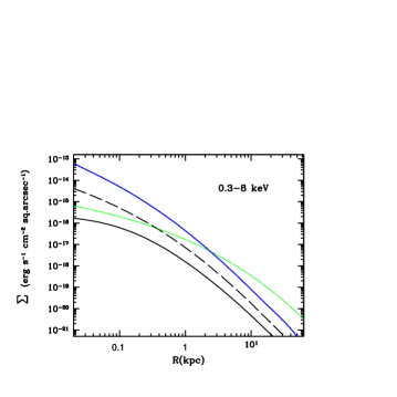
Figure 4: The surface brightness profile for the model in Fig. 3 (blue line), and for two other models whose hydrodynamical quantities are shown in the next Fig. 5, with the same line type, all at an age of 13 Gyr. The green line follows the optical profile of the testcase ETG, and is normalized to the emission of unresolved X-ray binaries, as 20% of their total collective luminosity (the unresolved fraction is $<25$% for a sample of local ETGs observed with $Chandra$, excluding the very hot gas rich ones; Kim10 ).

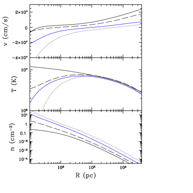
Figure 5: Radial trend of the main hydrodynamical quantities at a galaxy age of 13 Gyr, for the testcase ETG in Fig. 3 (blue lines), and for three galaxy models with the same $L_{B}$ and $\sigma_{c}$ except for the following differences: a SNIa’s rate increased by 20% (dashed line); $n=6$, $M_{*}/L_{B}=6.1$ (solid line); $n=4$, $M_{*}/L_{B}=8.5$ (dotted line). The corresponding gas luminosities are respectively $L_{X,ISM}=1.1\times 10^{39}$, $4\times 10^{38}$, $3.0\times 10^{40}$ erg s^-1. The brightness profiles of the models shown with a dashed and solid line are plotted in Fig. 4 (see Sect. 3.3).

Variations in the Testcase ETG and in $L_{X,ISM}$

See the full chapter (chapter 2 in Hot Interstellar Matter in Elliptical Galaxies, Springer, 2012; http://www.springer.com/astronomy/book/978-1-4614-0579-5)

4 The Nuclear Scale

Accretion to the center is commonly present, though from a small region, for the models in Fig. 5; therefore, this Section explores what modifications to the flow are expected from the addition of a central MBH. […] It is now clear that MBH feedback is unavoidable on cosmological timescales; however, for timescales much shorter than the cosmological one, and closer to the present epoch, it is not fully understood yet how it works in detail. It is then interesting to consider a few basics aspects of the flow behavior for models with a central MBH but neglecting feedback, as: how the flow is affected by the MBH gravity, the similarity of the accretion flow with a Bondi flow, how much accretion energy is expected, and how the picture outlined in the previous Sections is modified.

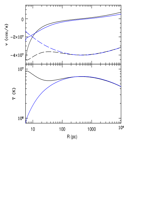
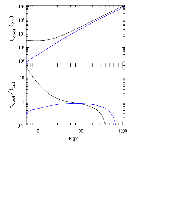
Figure 6: Left: the velocity and temperature profiles for the testcase ETG of Sect. 3.3 (in blue), and for the same galaxy model with a central MBH of mass $3.6\times 10^{8}M_{\odot}$ added (in black), at an age of 13 Gyr; the dashed lines show $-v_{s}$ for $\gamma=5/3$, for the two models respectively. Right: the cooling time and its ratio with the infall time, for the models on the left. See Sect. 4 for more details.

4.1 Gravitational Heating from the MBH and Comparison with the Bondi Accretion

The addition to the mass model of the testcase ETG (Sect. 3.3) of a central gravitating mass $M_{BH}=3.6\times 10^{8}M_{\odot}$, as predicted by the Magorrian relation, that remains constant with time, produces a flow that is not influenced by the MBH in the outer region; within the central $\sim 100$ pc, instead, the infall velocity and the temperature become larger (Fig. 6), the density lower, and the mass inflow rate to the center $\dot{M}_{in}$ smaller (from 0.12 to 0.06 $M_{\odot}$yr^-1 at a radius of 5 pc). The most relevant difference caused by the addition of the MBH is the higher gas temperature at the center; this is due to the heating of the gas produced by the sharp increase of the stellar velocity dispersion within the sphere of influence of the MBH (of radius of the order of $GM_{BH}/\sigma_{c}^{2}=20$ pc, where $\sigma_{c}$ is the velocity dispersion without the MBH; Fig. 7), and by the compression of the gas caused by the gravity of the MBH. The MBH heating succeeds in ”filling” the central ”hole” in temperature of the model without MBH, and it may even be able to create a small central peak in the gas temperature (Fig. 6). The difference in central temperature takes more time to establish for models with larger central gas density (as that with $n=4$ in Fig. 5), and it may even not take place within the present epoch. In models where the flow, without the MBH, keeps hot down to small radii (as that of the black solid lines in Fig. 5), the change in temperature is far less dramatic (an increase by 25% of the central temperature), and $\dot{M}_{in}$ remains substantially unchanged at very small values ($\dot{M}_{in}\sim 10^{-4}-10^{-3}\,M_{\odot}$yr^-1).

Another important property of the flow is the value of its velocity with respect to the sound velocity $v_{s}$, calculated for example for the adiabatic case ($\gamma=5/3$; $v_{s}=\sqrt{\gamma kT/\mu m_{p}}$), and also shown in Fig. 6. Without a MBH, in cases of ”cold” accretion as for the testcase ETG, the flow becomes supersonic close to the galactic center; with a MBH, accretion is hot and keeps subsonic, while the flow tends to reach the sound velocity at the innermost gridpoint (that, for this series of runs, has been put to 1 pc). In fact, in absence of momentum feedback, it is unavoidable for the flow to tend to the free fall velocity close to the MBH, where the potential energy per particle becomes larger than the thermal energy (and this is reproduced by the inner boundary condition of a vanishing thermodynamical pressure gradient). The MBH heating also causes the cooling time $t_{cool}$ to become much larger than the inflow time $t_{inf}$ within the central $\sim 100$ pc (Fig. 6). Both properties (the inflow velocity that tends to $v_{s}$, and $t_{cool}>>t_{inf}$) characterize also the Bondi (1952) solution for spherically symmetric accretion on a central point mass, from a nonrotating polytropic gas with given density and temperature at infinity, in the adiabatic case ($\gamma=5/3$). This fact provides some support to a commonly used procedure to estimate the MBH mass accretion rate of ETGs (e.g., L01 ; So ), that is the use of the analytic Bondi (1952) formula, replacing infinity with a fiducial accretion radius $r_{acc}=2GM_{BH}/v_{s}^{2}$ (Fra ), and calculating $v_{s}$ as close as possible to the MBH. This is not a trivial aspect since there are additional ingredients in the galactic flow that are not included in the Bondi (1952) analysis, but are accounted for by the simulations, as: 1) the presence of mass and energy sources, as the stellar mass losses and the SNIa’s heating; 2) the possibility of cooling; 3) the fact that $r_{acc}$ is not a true infinity point, since the gas experiences a pressure gradient there; 4) the contribution of the galactic potential added to that of the MBH. The simulations however have some limits too: for example, the discrete nature of the stellar distribution becomes important where the accretion time on the MBH ($t_{inf}\sim 10^{4}-10^{5}$ yrs from 10 pc, in the simulations) is comparable to (or lower than) the time required for the stellar mass losses to mix with the bulk flow (Mat90 ; PB ), or to the time elapsing between one SNIa event and the next (see also T10 ). Another limit is that some form of accretion feedback is also expected, as briefly outlined in the next Section.

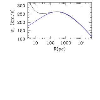
Figure 7: The projected stellar velocity dispersion profile for the galaxy model of the testcase ETG (Sect. 3.3, dotted line), and for the same model with a central MBH of mass $3\times 10^{8}M_{\odot}$ discussed in Sect. 4 (solid line). Both models have an aperture velocity dispersion of 260 km s^-1 within $R_{e}/8$.

4.2 The Importance of the Energy Output from Accretion

The mass inflow rates of the models in Fig. 5, with a central MBH added, range from $\dot{M}_{in}=4\times 10^{-4}$ (model with solid line) to $4\times 10^{-1}$ $M_{\odot}$yr^-1 (model with dotted line), at an inner gridpoint of 5 pc, at the present epoch. If totally accreted, the largest of these $\dot{M}_{in}$ releases an accretion power $L_{acc}\sim 0.1\dot{M}_{in}c^{2}=2\times 10^{45}$ erg s^-1 (Fra ), a large value that can have a significant impact on the surrounding hot ISM, depending on the fraction that can interact with the ISM and be transferred to it. $L_{acc}$ is mostly in radiative form at high mass accretion rates; more precisely, the radiative efficiency of the accreting material can be written in a general way as $\epsilon=0.2\times 100\dot{m}/(1+100\dot{m})$, where $\dot{m}=\dot{M}_{in}/\dot{M}_{Edd}$ is the Eddington-scaled accretion rate, and $\dot{M}_{Edd}=L_{Edd}/0.1c^{2}=2.2\times 10^{-8}M_{BH}(M_{\odot})\,\,\,M_{\odot}$yr^-1 (CO10 ). When $\dot{m}{\mathrel{\mathchoice{\lower 2.9pt\vbox{\halign{$\m@th\displaystyle\hfil#\hfil$\cr>\crcr\sim\crcr}}}{\lower 2.9pt\vbox{\halign{$\m@th\textstyle\hfil#\hfil$\cr>\crcr\sim\crcr}}}{\lower 2.9pt\vbox{\halign{$\m@th\scriptstyle\hfil#\hfil$\cr>\crcr\sim\crcr}}}{\lower 2.9pt\vbox{\halign{$\m@th\scriptscriptstyle\hfil#\hfil$\cr>\crcr\sim\crcr}}}}}0.01$, then $\epsilon\sim 0.1-0.2$, and $L_{acc}$ is mostly in radiative form; when $\dot{m}\ll 0.01$, then $\epsilon\sim 20\dot{m}$, as for radiatively inefficient accretion flows (Nar ), and the radiative output becomes negligible. In the low-$\epsilon$ regime, the output of accretion may be dominated by a kinetic form (BB ; Koe ; All ; Mer ). For example, from the energy input by accretion feedback to the hot coronae of a few nearby ETGs, with $\dot{M}_{in}$ calculated using the Bondi rate as described in Sect. 4 and $\dot{m}\ll 0.01$, it was found that $\sim 1/5$ of $L_{acc}$ is converted into jet power (All ). The lowest $\dot{m}$ among the models in Fig. 5 is $\sim 10^{-4}$, and then accretion is highly radiatively inefficient, but the largest is $\dot{m}=0.04$, […].

For a representative model [obtained with the high resolution simulations with radiative and mechanical feedback of Ciotti et al. (2010), similar to the testcase ETG (Sect. 2.3.3)], the duty cycle (the fraction of the time the AGN is in the ”on” state) is of the order of $10^{-2}$, for the past 5-7 Gyrs; outside the nuclear bursts, the flow behavior is similar to that described in Sect. 3 (CO10 ), with a major difference: the lower central gas density, due to the MBH heating (PCO ). […] The brightness profiles are then much less centrally peaked than those in Sect. 2.3.3. […]

In addition to this important (positive) effect on the surface brightness profile of the hot gas, how does AGN feedback modify the scenario outlined in the previous Sections? ETGs where $L_{SN}>L_{grav}^{-}$, and then already outflow-dominated, will not be affected by further sources of heating. For the other ETGs, the answer depends on how much energy from accretion is transferred to the hot ISM: if this energy is $>>L_{SN}$ then the scenario above will be modified, while if it is $<<L_{SN}$ it will be preserved. In general, it can be noted that the gas modeling based on realistic stellar and dark mass profiles, stellar mass loss and supernova rates and their secular evolution, without accretion feedback can already reproduce reasonably well the fundamental gas properties (e.g., trend of $L_{X,ISM}$ with $L_{B}$, wide variation in $L_{X,ISM}$, average gas temperature), therefore such modeling must catch the bulk of the origin and evolution of the hot gas in ETGs. Moreover, even in the context of feedback modulated gas flow evolution, the hot gas content at the present epoch, seem still sensitive to the structural galaxy parameters, in the same sense as described in Sects. 2.3 and 3 (Ciotti & Ostriker, this volume; PCO ). Finally, the modeling without feedback – if any – shows the need for gas accretion from outside or confinement (Sect. 3); the nuclear energy input should then mostly readjust the internal gas structure, without causing major degassing at later epochs. The measure in which activity affects the gas content is yet to be established observationally; so far, exploiting $Chandra$ resolution, it has just been shown that the nuclear X-ray luminosities of ETGs correlate only weakly with their gas luminosity (P10 ).

5 Gas Flows and Galactic Shape, Rotation, Stellar Profile

In Sect. 3 it was shown how the gas content of an ETG is sensitive to changes regarding the stellar and dark mass components that are in fact allowed for by observations (see, e.g., the scatter around the fundamental scaling laws of ETGs), and by modeling (see, e.g., how model ETGs lying on the Fundamental Plane can be built with different $\cal{R}$ and $\beta$, RC93 and Sect. 3.3). This holds even at fixed $L_{B}$, so to account for a significant part of the large observed $L_{X,ISM}$ variation. Below we consider the effects on the hot gas content produced by additional variations in the galactic structure that are observed and have not been considered above, such as the galactic shape, the amount of rotation in the stellar motions, and the central stellar profile.

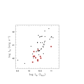
Figure 8: The total X-ray emission (from $ROSAT$ PSPC observations, OS ) versus the galactic blue luminosity $L_{B}$ (from total B-magnitudes in the Hyperleda catalog and distances in OS ) for a sample of ETGs with measured optical flattening and stellar rotation (P97 ). Galaxies with high flattening ($b/a<0.6$) are marked with a red circle (see Sect. 5.1 for more details).

5.1 Galactic Shape and Rotation

Soon after the first large sample of ETGs with known X-ray emission was built from $Einstein$ observations, it was found that the hot gas retention capability is related to the intrinsic galactic shape: on average, at any fixed $L_{\rm B}$, rounder systems show larger total X-ray emission $L_{\rm X}$ and $L_{\rm X}/L_{\rm B}$ than flatter elliptical and S0 systems Esk . The relationship defined by $L_{\rm X}/L_{\rm B}$ is stronger than that defined by $L_{\rm X}$. Moreover, galaxies with axial ratio $b/a$ close to unity span the full range of $L_{\rm X}$, while flat systems all have $L_{\rm X}{\mathrel{\mathchoice{\lower 2.9pt\vbox{\halign{$\m@th\displaystyle\hfil#\hfil$\cr<\crcr\sim\crcr}}}{\lower 2.9pt\vbox{\halign{$\m@th\textstyle\hfil#\hfil$\cr<\crcr\sim\crcr}}}{\lower 2.9pt\vbox{\halign{$\m@th\scriptstyle\hfil#\hfil$\cr<\crcr\sim\crcr}}}{\lower 2.9pt\vbox{\halign{$\m@th\scriptscriptstyle\hfil#\hfil$\cr<\crcr\sim\crcr}}}}}10^{41}$ erg s^-1 (see, e.g., Fig. 8). A similar result holds for the ”diskiness” or ”boxiness” property of ETGs, that measures the deviation of the isophotal shape from a pure elliptical one (Ben ; KB ). This property is described by the $a_{4}/a$ parameter, in a way that disky ($a_{4}>0$) ETGs show isophotes distorted in the sense of a disk, and boxy ($a_{4}<0$) ETGs have isophotal distortions in the sense of a box. Disky systems are also generally flattened by rotation, while boxy ones have various degrees of velocity anisotropy (see also Pas ). Boxy ETGs cover the whole observed range of $L_{\rm X}$, while disky ETGs are less X-ray luminous on average (Ben ; Esk ); this result is not produced only by disky galaxies having a lower average galactic luminosity, with respect to boxy ETGs, since it holds even in the range of $L_{B}$ where the two types overlap (P99b ). The relationship between $L_{\rm X}$ and $a_{4}/a$ was reconsidered, confirming the above trends, for the $ROSAT$ PSPC sample (EO ).

Figure 9: The total X-ray emission versus the galactic luminosity $L_{B}$ (both determined as in Fig. 8); galaxies with $v_{\rm rot}/\sigma_{\rm c}>0.5$ are marked with a red symbol (see Sect. 5.1 for more details).

There seems then to be a dependence of the hot gas content on the galactic shape, measured by either $\epsilon=1-b/a$ or $a_{4}/a$. Since flatter and disky systems also possess, on average, higher rotation levels (bt87 ), the influence on the hot gas of both the shape of the potential well and of the stellar rotation was called into question. The gas in ETGs that are in part rotationally supported may have a lower “effective” binding energy per unit luminosity compared to the gas in non-rotating ones (a lower effective $L_{grav}^{-}/L_{\rm B}$ ratio, in the notation of Sect. 2.3; see also Sect. 5.1 below), and then rotating ETGs may be more prone to host outflowing regions. For this reason, the effects on $L_{\rm X}$ of the ellipticity $\epsilon$ of the stellar distribution and of stellar rotation were studied for a sample of 52 ETGs with known $L_{\rm X}$, maximum rotational velocity of the stars $v_{\rm rot}$, and central stellar velocity dispersion $\sigma_{\rm c}$ (P97 ). […]p The gas content can be high only for values of $v_{\rm rot}/\sigma_{\rm c}{\mathrel{\mathchoice{\lower 2.9pt\vbox{\halign{$\m@th\displaystyle\hfil#\hfil$\cr<\crcr\sim\crcr}}}{\lower 2.9pt\vbox{\halign{$\m@th\textstyle\hfil#\hfil$\cr<\crcr\sim\crcr}}}{\lower 2.9pt\vbox{\halign{$\m@th\scriptstyle\hfil#\hfil$\cr<\crcr\sim\crcr}}}{\lower 2.9pt\vbox{\halign{$\m@th\scriptscriptstyle\hfil#\hfil$\cr<\crcr\sim\crcr}}}}}0.4$, while modest or low gas contents, as log[$L_{\rm X}$(erg s${}^{-1})/L_{\rm B}(L_{B,\odot})]{\mathrel{\mathchoice{\lower 2.9pt\vbox{\halign{$\m@th\displaystyle\hfil#\hfil$\cr<\crcr\sim\crcr}}}{\lower 2.9pt\vbox{\halign{$\m@th\textstyle\hfil#\hfil$\cr<\crcr\sim\crcr}}}{\lower 2.9pt\vbox{\halign{$\m@th\scriptstyle\hfil#\hfil$\cr<\crcr\sim\crcr}}}{\lower 2.9pt\vbox{\halign{$\m@th\scriptscriptstyle\hfil#\hfil$\cr<\crcr\sim\crcr}}}}}30.2$, are independent of the degree of rotational support. Recently, for the ETGs of the $SAURON$ sample, the relationship between soft X-ray emission and rotational properties was investigated again (Sar ), confirming that slowly rotating galaxies can exhibit much larger luminosities than fast-rotating ones. As for the axial ratio and the isophotal parameter $a_{4}$, the trend of $L_{\rm X}/L_{\rm B}$ with $v_{\rm rot}/\sigma_{\rm c}$ is not produced by the correlation between $L_{\rm X}$ and $L_{\rm B}$: ETGs with high $v_{\rm rot}/\sigma_{\rm c}$ cover substantially the same large range in $L_{\rm B}$ as the whole sample (Fig. 9 ).

In conclusion, rotation seems to have an effect similar to that of shape, and $L_{X}$ and $L_{X}/L_{B}$ show a similar trend with respect to axial ratio, diskiness, and rotation: their variation is large for round, boxy and slowly-rotating systems, while it keeps below a threshold for flatter, disky and high-rotation systems. From observations it remains then undecided which one between axial ratio, diskiness, and rotation is responsible for the trend; more insights is given by the theoretical and numerical analysis discussed below.

A Theoretical and Numerical Investigation

The impact of stellar rotation and galactic shape on the hot gas content was also addressed with theoretical and numerical studies (CP96 ; BM96 ; DC ). In principle, the lower gas content of flatter systems could be due to the mass distribution itself, or to a higher rotational level that decreases the effective potential. An analytic investigation showed that flatter systems are less able to retain hot gaseous halos than rounder ones of the same $L_{\rm B}$, due to the effect of the shape more than that of a larger rotational level (CP96 ). The investigation reconsidered the global estimate of the energy budget of the gas introduced in Sect. 2.3, generalizing it for flows in flat and rotating galaxy models. The classical scalar virial theorem for a stellar distribution interacting with a dark matter potential can be written as $2T+\Pi=|W|$, where $\Pi$ and $T$ are the kinetic energies associated respectively with the stellar random and ordered motions, and $|W|$ is the potential energy of the stellar component plus the virial interaction energy of the stars with the dark halo. For a fixed total mass and mass distribution (i.e., a fixed $|W|$), the amount of rotational streaming energy $T$ can formally vary from zero to a maximum that depends on the galaxy structure (CP96 ); in the notation of Sect. 2.3, the power $L_{rot}$ related to rotational streaming is $L_{rot}=\dot{M}_{*}\,T/M_{*}$, while that related to random motions is $L_{\sigma}=0.5\dot{M}_{*}\,\Pi/M_{*}$. How does $L_{rot}$ enter the energy budget of the gas, for example in Eq. 9, for a fixed $|W|=2\,M_{*}\,(L_{rot}+L_{\sigma})\,/\,\dot{M}_{*}$ ? In an extreme case, the whole effect of the ordered motion is to produce a change in the effective potential experienced by the gas, if for example the galactic corona is rotating with the same rotation velocity as the stars; in this case $L_{rot}$ is to be subtracted from $L_{grav}^{-}$. In the opposite extreme case, all the kinetic energy of the gas, from random and from ordered motions, is eventually thermalized; then $L_{rot}$ is to be added to $L_{SN}$ and $L_{\sigma}$, in the denominator of Eq. 9. The real behavior, lying between the two extreme cases, can be parameterized re-writing Eq. 9 as

$${L_{grav}^{-}-\alpha L_{rot}\over L_{SN}+L_{\sigma}+(1-\alpha)L_{rot}}$$ (11)

with $0\leq\alpha\leq 1$. If $\alpha=0$, the thermalization of $L_{rot}$ is complete, and since the kinetic energy of stellar motions ($L_{\sigma}+L_{rot}$) will be lower than $L_{SN}$, then Eq. 11 coincides with Eq. 9. If instead $\alpha=1$, there is no thermalization of $L_{rot}$, the decrease of $L_{grav}^{-}$ is maximum, and the effect of rotation is maximum. However, it is found that the role of rotation remains minor, because it can change Eq. 11 by only a few per cent: the variation of Eq. 11, between the null and the maximum $L_{rot}$ allowed by realistic galaxy models, is small, even for $\alpha=1$ ($<10$%; CP96 ). Instead, variations of more significant amount that can make the gas significantly less bound (a decrease in $L_{grav}^{-}$ of $\sim 20$%) can be produced by a change in the galaxy structure, as a reasonable flattening of a round system at fixed $L_{\rm B}$. Therefore, S0s and non-spherical ellipticals are less able to retain hot gaseous haloes than are rounder systems of the same $L_{\rm B}$, and more likely to host outflowing regions.

The results of the purely energetical approach above were tested with numerical studies of gas flows. Two-dimensional simulations for oblate ETGs, with different amounts of ordered and disordered kinetic energies, were carried out for gas in the inflow state (BM96 ). In this investigation $L_{\rm X}$ is reduced in rotating models, because the gas cools on a disk before entering the galactic core region, and then $L_{grav}^{+}$ (Eq. 6) is reduced; since rotation increases on average with flatness, rotation would be the underlying cause of the X-ray underluminosity of flat objects. However, the massive, rotationally supported, and extended cold disk that forms in the equatorial plane, due to mass and angular momentum conservation, and comparable in size to the effective radius, is not observed; also, the resulting X-ray images should be considerably flattened towards the equatorial plane out to an optical effective radius or beyond, a phenomenon that is small or absent (Han ). Other authors (DC ) performed two-dimensional numerical simulations of gas flows for flat systems, but allowing for the gas to be outflowing. The flows then developed a partial wind in flat ETGs that, if spherical, would be in inflow. In this way, the models accumulate negligible amounts of cold gas on a central disk. Rotation could also decrease the X-ray emission (of a factor of two or less), because it favoured the wind. In this scenario, then, flat models, rotating or not, can be significantly less X-ray luminous than spherical ones of the same $L_{\rm B}$, because they are in partial wind when the spherical ones are in inflow; rotation has an additional but less important effect.

5.2 The Central Stellar Profile

[…] Interestingly, the radio luminosity $L_{R}$ shows the same behavior as the total soft X-ray emission with respect to the inner stellar light profile: cusp ETGs are confined below a threshold in $L_{R}$, while core ones span a large range of $L_{R}$ (Ben ; CB ; P10 ). Core systems can then reach the highest $L_{R}$ and possess a conspicuous radio activity cycle, while in cusp galaxies the radio emission keeps smaller, likely because of a rapid jet failure due to the lack of a dense confining medium, or a smaller duty cycle (P10 and references therein).

- (1) Acreman, D.M., Stevens, I. R., Ponman, T. J., Sakelliou, I., MNRAS, 341, 1333 (2003)
- (2) Allen, S.W., et al., MNRAS 372, 21 (2006)
- (3) Athey, A., Bregman, J., Bregman, J., Temi, P., Sauvage, M., ApJ, 571, 272 (2002)
- (4) Bender, R., Surma P., Doebereiner S., Moellenhoff C., Madejsky R., A&A, 217, 35 (1989)
- (5) Bernardi, M., Sheth, R. K., Annis, J. B., et al., AJ, 125, 1866 (2003)
- (6) Bertin, G., Toniazzo, T., ApJ , 451, 111 (1995)
- (7) Binney, J., Tremaine, S., Galactic Dynamics, PUP (1987)
- (8) Blandford, R. D., Begelman, M. C., MNRAS, 303, L1 (1999)
- (9) Bondi, H., MNRAS, 112, 195 (1952)
- (10) Boroson, B., Kim, D.W., Fabbiano, G., ApJ, 729, 12 (2011)
- (11) Brassington, N. J., Ponman, T.J., Read, A.M., MNRAS, 377, 1439 (2007)
- (12) Bregman, J.N., Parriott, J.R., ApJ , 699, 923 (2009)
- (13) Brighenti, F., Mathews W. G., ApJ, 470, 747 (1996)
- (14) Brighenti, F., Mathews, W.G., ApJ , 495, 239 (1998)
- (15) Brown, B. A., Bregman J. N., ApJ, 539, 592 (2000)
- (16) Capetti, A., Balmaverde, B., A&A, 440, 73 (2005)
- (17) Cappellari, M., Bacon, R., Bureau, M., et al., MNRAS, 366, 1126 (2006)
- (18) Cappellaro, E., Evans, R., Turatto, M., A&A, 351, 459 (1999)
- (19) Churazov, E., Sazonov, S., Sunyaev, R., Forman, W., Jones, C., Böhringer, H., MNRAS, 363, L91 (2005)
- (20) Ciotti, L., D’Ercole, A., Pellegrini, S., Renzini, A., ApJ , 376, 380 (1991)
- (21) Ciotti, L., Pellegrini, S., MNRAS, 255, 561 (1992)
- (22) Ciotti, L., Pellegrini, S., MNRAS, 279, 240 (1996)
- (23) Ciotti, L., Ostriker, J.P., ApJ , 665, 1038 (2007)
- (24) Ciotti, L., Pellegrini, S., MNRAS, 387, 902 (2008)
- (25) Ciotti, L., Ostriker, J.P., Proga, D., ApJ , 717, 708 (2010)
- (26) Côté, P., et al., ApJS, 165, 57 (2006)
- (27) Croton, D.J., Springel, V., White, S.D.M., et al., MNRAS, 365, 11 (2006)
- (28) David, L. P., Forman, W., Jones, C., ApJ, 359, 29 (1990)
- (29) David, L. P., Forman, W., Jones, C., ApJ, 369, 121 (1991)
- (30) David, L.P., Jones, C., Forman, W., Vargas, I.M., Nulsen, P., ApJ, 653, 207 (2006)
- (31) Davies, R.L., Efstathiou, G., Fall, S.M., Illingworth, G., Schechter, P.L., ApJ, 266, 41 (1983)
- (32) D’Ercole, A., Ciotti, L., ApJ, 494, 535 (1998)
- (33) D’Ercole, A., Ciotti, L., Recchi, S., ApJ, 533, 799 (2000)
- (34) Diehl, S., & Statler, T. S., ApJ, 668, 150 (2007)
- (35) Diehl, S., & Statler, T. S., ApJ, 680, 897 (2008)
- (36) Diehl, S., & Statler, T. S., ApJ, 687, 986 (2008)
- (37) Ebisuzaki, T., Makino, J., Tsuru, T.G., et al., ApJ, 562, L19 (2001)
- (38) Ellis, S.C., O’Sullivan, E., MNRAS, 367, 627 (2006)
- (39) Eskridge, P. B., Fabbiano G., Kim D., ApJ, 442, 523 (1995)
- (40) Fabbiano, G., ARA&A, 27, 87 (1989)
- (41) Fabbiano, G., Schweizer, F., ApJ, 447, 572 (1995)
- (42) Faber, S. M., Gallagher, J. S., ApJ, 204, 365 (1976)
- (43) Faber, S. M., Tremaine, S., Ajhar, E.A., et al., AJ, 114, 1771 (1997)
- (44) Fabian, A.C., Canizares, C.R., Nature, 333, 829 (1988)
- (45) Ferrarese, L., Ford, H., Space Sci. Rev., 116, 523 (2005)
- (46) Finoguenov, A., Jones, C., ApJ, 547, L107 (2001)
- (47) Forman, W., Nulsen, P., Heinz, S., et al. ApJ, 635, 894 (2005)
- (48) Frank, J., King, A., & Raine, D., Accretion Power in Astrophysics, Cambridge: CUP (2002)
- (49) Fukazawa, Y., et al., ApJ, 636, 698 (2006)
- (50) Graham, A. W., ApJ, 613, L33 (2004)
- (51) Greggio, L., A&A, 441, 1055 (2005)
- (52) Greggio, L., MNRAS, 406, 22 (2010)
- (53) Gualandris, A., Merritt, D., ApJ, 678, 780 (2008)
- (54) Hanlan, P.C., Bregman, J.N., ApJ, 530, 213 (2000)
- (55) Helsdon, S.F., et al., MNRAS, 325, 693 (2001)
- (56) Ho, L.C., ARA&A, 46, 475 (2008)
- (57) Humphrey, P.J., Buote, D.A., ApJ, 639, 136 (2006)
- (58) Jeltema, T.E., Binder, B., Mulchaey, J.S., ApJ, 679, 1162 (2008)
- (59) Kauffmann, G., Heckman, T. M., MNRAS, 397, 135 (2009)
- (60) Kim, D.W., Fabbiano, G., ApJ, 586, 826 (2003)
- (61) Kim, D.W., Kim, E., Fabbiano, G., Trinchieri, G., ApJ, 688, 931 (2008)
- (62) Körding, E.G., Fender, R.P., Migliari, S., MNRAS, 369, 1451 (2006)
- (63) Komatsu, E., Dunkley, J., Nolta, M. R., et al., ApJS, 180, 330 (2009)
- (64) Kormendy, J., Bender, R., ApJ, 464, L119 (1996)
- (65) Kormendy, J., Fisher, D.B., Cornell, M.E., Bender, R., ApJS, 182, 216 (2009)
- (66) Laine, S., van der Marel, R.P., Lauer, T.R., et al., AJ, 125, 478 (2003)
- (67) Lauer, T. R., et al. AJ, 129, 2138 (1995)
- (68) Lauer, T. R., et al. ApJ, 664, 226 (2007)
- (69) Li, W., et al. MNRAS, 412, 1473 (2011)
- (70) Loewenstein, M., Mathews, W.G., ApJ 319, 614 (1987)
- (71) Loewenstein, M., et al., ApJ, 555, L21 (2001)
- (72) MacDonald, J., Bailey, M. E., MNRAS, 197, 995 (1981)
- (73) Mannucci, F., et al., A&A, 433, 807 (2005)
- (74) Maoz, D., et al., ApJ, 412, 1508 (2011)
- (75) Maraston, C., MNRAS, 362, 799 (2005)
- (76) Mathews, W.G., AJ 97, 42 (1989)
- (77) Mathews, W.G., ApJ 354, 468 (1990)
- (78) Matsushita, K., ApJ, 547, 693 (2001)
- (79) Memola, E., et al., A&A, 497, 359 (2009)
- (80) Merloni, A., Heinz, S., MNRAS, 381, 589 (2007)
- (81) Milosavljevic, M., Merritt, D., Rest, A., van den Bosch, F.C., MNRAS, 331, L51 (2000)
- (82) Nagino, R., Matsushita, K., A&A, 501, 157 (2009)
- (83) Napolitano, N. R., Romanowsky, A. J., Capaccioli, M., et al., MNRAS, 411, 2035 (2011)
- (84) Narayan, R., Yi, I., ApJ, 452, 710 (1995)
- (85) Navarro, J. F., Frenk, C. S., White, S. D. M., ApJ , 490, 493 (1997)
- (86) Omma, H., Binney, J., Bryan, G., & Slyz, A., MNRAS, 348, 1105 (2004)
- (87) O’Sullivan, E., Forbes D. A., Ponman T. J., MNRAS, 328, 461 (2001)
- (88) O’Sullivan, E., Ponman, T.J., Collins, R.S., MNRAS 340, 1375 (2003)
- (89) Parriott, J.R., Bregman, J.N., ApJ , 681, 1215 (2008)
- (90) Pasquali, A., van den Bosch, F. C., Rix, H.-W., ApJ, 664, 738 (2007)
- (91) Pellegrini, S., Held E. V., Ciotti L., MNRAS, 288, 1 (1997)
- (92) Pellegrini, S., Ciotti, L., A&A, 333, 433 (1998)
- (93) Pellegrini, S., A&A, 343, 23 (1999)
- (94) Pellegrini, S., A&A, 351, 487 (1999)
- (95) Pellegrini, S., MNRAS, 364, 169 (2005)
- (96) Pellegrini, S., ApJ , 624, 155 (2005)
- (97) Pellegrini, S., et al., ApJ , 667, 731 (2007)
- (98) Pellegrini, S., Ciotti, L., Ostriker, J. P., ApJ, 744, 21 (2012)
- (99) Pellegrini, S., ApJ , 717, 640 (2010)
- (100) Pellegrini, S., ApJ , 738, 57 (2011)
- (101) Peterson, J. R., Fabian, A. C., PhR, 427, 1 (2006)
- (102) Pizzolato, F., Soker, N., MNRAS, 408, 961 (2010)
- (103) Quataert, E., Narayan, R., ApJ, 528, 236 (2000)
- (104) Read, A.M., Ponman, T.J., MNRAS, 297, 143 (1998)
- (105) Renzini, A., Ciotti, L., ApJ, 416, L49 (1993)
- (106) Renzini, A., Ciotti, L., D’Ercole, A., Pellegrini, S., ApJ, 419, 52 (1993)
- (107) Saglia, R. P., Bertin, G., Stiavelli, M., ApJ, 384, 433 (1992)
- (108) Sarazin, C.L., White, R.E.III, ApJ , 320, 32 (1987)
- (109) Sarazin, C.L., White, R.E.III, ApJ , 331, 102 (1988)
- (110) Sarazin, C.L., Ashe, G.A., ApJ , 345, 22 (1989)
- (111) Sarzi, M., Shields, J.C., Schawinski, K., et al., MNRAS, 402, 2187 (2010)
- (112) Sharon, K., Gal-Yam, A., Maoz, D., et al., ApJ, 718, 876 (2010)
- (113) Shen, J., Gebhardt, K., ApJ , 711, 484 (2010)
- (114) Soria, R., et al., ApJ, 640, 126 (2006)
- (115) Sun, M., et al., ApJ , 657, 197 (2007)
- (116) Sun, M., Voit, G. M., Donahue, M., Jones, C., Forman, W., Vikhlinin, A., ApJ , 693, 1142 (2009)
- (117) Tabor, G., Binney, J., MNRAS, 263, 323 (1993)
- (118) Tang, S., Wang, Q. D., Lu, Y., Mo, H. J., MNRAS, 392, 77 (2009)
- (119) Tang, S., Wang, Q.D., MNRAS, 408, 1011 (2010)
- (120) Tonry, J., Dressler, A., Blakeslee, J.P., et al., ApJ, 546, 681 (2001)
- (121) Trinchieri, G., Pellegrini, S., Fabbiano, G., et al., ApJ 688, 1000 (2008)
- (122) Trujillo, I., et al., 127, 1917 (2004)
- (123) Weijmans, A.M., Cappellari, M., Bacon, R., et al., MNRAS, 398, 561 (2009)