Satisfiability thresholds beyond $k-$XORSAT

Abstract

We consider random systems of equations $x_{1}+\dots+x_{k}=a,$ $0\leq a\leq 2$ which are interpreted as equations modulo $3.$ We show for $k\geq 15$ that the satisfiability threshold of such systems occurs where the $2-$core has density $1.$ We show a similar result for random uniquely extendible constraints over $4$ elements. Our results extend previous results of Dubois/Mandler for equations $\mod 2$ and $k=3$ and Connamacher/Molloy for uniquely extendible constraints over a domain of $4$ elements with $k=3$ arguments.

Our proof technique is based on variance calculations, using a technique introduced Dubois/Mandler. However, several additional observations (of independent interest) are necessary.

1 Introcuction

1.1 Contribution

Often constraints are equations of the type $f(x_{1},\dots,x_{k})=a$ where $a$ is an element of the domain considered and $f$ is a $k-$ary function on this domain, for example addition of $k$ elements. Given a formula, which is a conjunction of $m$ constraints over $n$ variables we want to find a solution. It is natural to assume that $f$ has the property: Given $k-1$ arguments we can always set the last argument such, that the constraint becomes true. In this case we can restrict attention to the $2-$core. It is obtained by iteratively deleting all variables which occur at most once. Thus it is the maximal subformula in which each variable occurs at least twice.

We consider the random instance $F(n,p):$ Each equation over $n$ variables is picked independently with probability $p;$ the domain size $d$ and the number of slots per equation $k$ is fixed. We consider the case $p=c/n^{k-1}$ and the number of constraints is linear in $n$ whp. (with high probability, that is probability $1\,-\,o(1),n$ large. ) The density of a formula is equal to the number of equations divided by the number of variables. The following is well known:

Fact 1 ([2])

1. Conditional on the number of variables $n^{\prime}$ and equations $m^{\prime}$ of the $2-$core the $2-$core is a uniform random member of all formulas where each variable occurs at least twice.
2. There exist $n^{\prime}=n^{\prime}(c)$ and $m^{\prime}=m^{\prime}(c)$ such that the number of variables of the $2-$core is $n^{\prime}(1+o(1))$ and the number of equations $m^{\prime}(1+o(1))$ whp.
3. There exists a $T$ such that whp. for $c\leq T-\varepsilon$ the $2-$core has density $\leq 1-\varepsilon$ and for $c\geq T+\varepsilon$ the $2-$core has density $\geq 1+\varepsilon.$ $T$ is determined as the solution of an analytical equation.

The expected number of solutions of the $2-$core is $d^{n-m},n$ the number of variables, $m$ the number of equations. When the $2-$core has density $\geq 1+\varepsilon$ whp. no solution exists. This holds in particular when the density of $F(n,p)$ itself is $\geq 1+\varepsilon.$ The formulas considered here always have density $<1.$ In seminal work Dubois and Mandler [8] consider equations $\mod 2:$ $x_{1}\,+\,\dots\,+\,x_{k}=a,$ $0\leq a\leq 1,k=3.$ They show satisfiability whp. when the $2$-core has density $\leq 1-\varepsilon.$ For larger $k\geq 15$ a full proof for this result is given in [5], Appendix C . Thus $T/n^{k-1}$ is the threshold for unsatisfiability in this case.

It is a natural conjecture that the same threshold applies to equations as discussed initially (and to some other types.) However, it seems difficult to prove the conjecture in some generality. One of the difficulties seems to be that we have $2$ parameters $k$ and $d.$ We make some progress towards this conjecture. We show it for equations $\mod 3.$ (The result is for $k>15,$ but we think it mainly technical to get it for all $k\geq 3.$)

Theorem 2

Let $F(n,p)$ be the random set of equations $\mod 3:$ $x_{1}+\dots+x_{k}\,=\,a,\,0\leq a\leq 2,$ $x_{1}+\dots+x_{k}$ an ordered $k-tuple$ of variables. If $p<(T-\varepsilon)/n^{k-1}$ $F(n,p)$ is satisfiable whp. for $k>15.$

The main task is to show that a $2-$core of density $\leq 1-\varepsilon$ has a solution with probability $>\varepsilon>0$ . Our proof starts as Dubois/Mandler: Let $X$ be the number of satisfying assignments of the $2-$core. Its expectation is $\geq d^{\varepsilon n},d=3.$ We show that $E[X^{2}]\leq O(E[X])^{2}.$ This implies (by Cauchy-Schwartz (or Paley-Zygmund) inequality) that the probability to have a solution is $\geq\varepsilon>0.$ By Fact 1 $F(n,p)$ has a solution with the same probability. We apply Friedgut-Bourgain’s Theorem to $F(n,p)$ to show that unsatisfiability has a sharp threshold. By this the probability becomes $1-o(1).$ In [9] Friedgut-Bourgain is applied to the $\mod 2-$case. It seems that our proof for the $\mod 3-$case is somewhat simpler (and applies to the $\mod 2-$case and other cases.)

To determine $E[X^{2}]$ Dubois/Mandler apply Laplace Method (one ingredient: bounding a sum through its maximum term.) The main difficulty is to bound a real function of several arguments from above. They show that their function has only one local maximum. We proceed by the same method, but substantial changes are necessary for $k>3.$

First, we observe (cf. [5], Appendix C) that the function in question is $\leq$ the infimum with respect to certain other parameters. This is based on generating functions: If $f(x)=\sum c_{k}x^{k}$ then $c^{k}\leq f(a)/a^{k},\,a>0,c_{i}\geq 0$ (a method rarely used in the area, a notable exception is [16].) Thus to bound the maximum from above we need to find suitable parameters and show that the value with respect to these parameters is less than the required upper bound . (This leads to involved, but elementary calculus. )

To make this approach work we need appropriate generating functions: $X=X_{a_{1}}+\dots X_{a_{3^{n}}},$ where $X_{a_{i}}$ is the indicator random variable of the event that assignment $a_{i}$ makes the formula true. Then $X^{2}=\sum_{a}\sum_{b}\,X_{a}X_{b}.$ To get $E[X^{2}]$ we need to determine Prob$[X_{a}X_{b}=1].$ To this end we observe that the equation $x_{1}+\dots+x_{k}=c$ which is true under $a$ is true exactly under those assignments $b$ such that $0k_{0}+1k_{1}+2k_{2}=0\mod 3,$ and $k_{i}$ is the number of slots of $x_{1}+\dots+x_{k}$ filled with a variable $x$ with $b(x)=a(x)+i.$ Thus there are $\sum_{k_{1}=k_{2}\mod 3}{k\choose k-k_{1}-k_{2},k_{1},k_{2}}$ different ways in which an equation can become true under $a,b.$ The following generating function allows us to deal with these possibilities analytically. With $\bf w_{1}\,=\,\exp(2\pi\i/3)$ the primitive third root of unity and $\bf w_{2}\,=w_{1}^{2}$ we define $r(x_{0},x_{1},x_{2})=\frac{1}{3}\left[(x_{0}\,+\,x_{1}\,+\,x_{2})^{k}\,+\,(x_{0}\,+\,{\bf w_{1}}x_{1}+{\bf w_{2}}x_{2})^{k}\,+\,(x_{0}\,+\,{\bf w_{2}}x_{1}\,+\,{\bf w_{1}}x_{2})^{k}\right]$
then Coeff$[x_{1}^{k_{1}}x_{2}^{k_{2}},r(1,\,x_{1},\,x_{2})]={k\choose k-k_{1}-k_{2},k_{1},k_{2}}$ if $k_{1}=k_{2}\mod 3$ and $0$ otherwise (easy from properties $\bf w_{j}.)$ In the $\mod 2-$case we use $1/2\left[(1+x)^{k}\,\,+\,\,(1-x)^{k}\right]$ instead [5], Appendix C.

With the motivation to get an exact threshold of unsatisfiability for a type of constraint whose worst-case complexity is NP-complete, Connamacher/Molloy [6] see also the very recent [17] introduce uniquely extendible constraints. A $k-$ary uniquely extendible constraint is a function from $D^{k}$ to true, false with the property: Given values from $D$ for any $k-1$ argument slots there is exactly one value for the remaining slot which makes the constraint true. (The $k>8$ in the following result can be eliminated at the price of some additional technical effort.)

Theorem 3

Let $F(n,p)$ be the random formula of uniquely extendible constraints: Each constraint is a random $k-$tuple of variables and a $k-$ary uniquely extendible constraint over $D$ and we pick with probability $p.$ For $|D|=4$ and $p<(T-\varepsilon)/n^{k-1}$ $F(n,p)$ is satisfiable whp. for $k>8.$

The threshold $T/n^{k-1}$ is proved for $k=3$ and $|D|=4$, cf. [17] remark following Theorem 8. Our proof uses the technique as in the $\mod 3-$case, however the details are different. One of the contributions making is the generating polynomial
$p(x)=\frac{1}{d}\left[(1+x)^{k}+(d-1)(1-\frac{x}{d-1})^{k}\right],$ as $r(x_{0},x_{1},x_{2})$ above, not used before.

1.2 Motivation

Many computational problems can be naturally formulated as conjunctions of constraints. And we are interested to find a solution of this conjunction. Algorithmic properties of these conjunctions are considered in theoretical research (with remarkable results e. g. in the realm of approximation[3]) and applied research, e. g. [18]. An additional aspect is the investigation of conjunctions of randomly picked constraints; [7] is a fundamental study here. Propositional formulas in $k$-conjunctive normalform provide an example which has lead to a rich literature e. g. [1]. One of the characteristic properties of this research is that its findings can often be related to experimental work by running algorithms on randomly generated instances.

One of the aspects of random formulas is a threshold phenomenon: If the number of constraints of a conjunction picked is less than a threshold value the conjunction is typically satisfiable, if it is more we get unsatisfiability whp. Moreover instances picked close to the threshold seem to be algorithmically hard, thus being candidate test cases for algorithms. The threshold phenomenon and the possibility to investigate it by experiments causes physics to become interested in the area e. g. [11]. On the other hand, physical approaches lead to new algorithms and classical theoretical computer science research, e. g. [12].

One of the major topics is to determine the value of the threshold in natural cases. A full solution even in the natural $k-$CNF SAT case has not been obtained, but many partial results, [1] for $k=3.$ Note that $k-$CNF does not have the unique extendability property as possessed by the constraints considered here. And it seems to be a major open problem to get the precise threshold for constraints without unique extendibility and not similar to $2-$CNF. A mere existence result is the Friedgut-Bourgain theorem [13]. Based on this theorem thresholds for formulas of constraints over domains with more than $2$ elements are considered in [7]. Ordering constraints are considered in [14], only partial results towards a threshold can be proven. In order to get definite threshold results further techniques are required. Therefore it is a useful effort to further develop the techniques with which thresholds can be proven. This is the general contribution of this paper.

A notable early exception, in that the precise threshold can be proven is the $\mod 2-$case considered above. Historically [8] is the first paper which uses variance calculation based on Laplace method in this area. Subsequently, for $k-$CNF SAT this method has lead to substantial progress in [15]. The contribution here is that $\mod 2-$proof can be refined and extended to cover other cases based on observations of independent interest. Note that random sparse linear systems over finite fields are used to construct error correcting codes, e. g. [19] or [20], motivating the $\mod 3-$case. A very recent study of the $\mod 2-$ case is [21]. More literature can be found in [10], but precise threshold results have not been obtained.

1.3 Contents

I. Equations modulo $3$
1. Notation and basics
2. Outline of the proof of Theorem 5
3. Proof of Theorem 9
3.1 Proof of Lemma 17
3.2 Proof of Lemma 18
3.3 Proof of Lemma 19
3.4 Proof of Lemma 20
4. Proof of Theorem 15
5. Remaining proofs
5.1 Local limit consideration
5.2 The sharp threshold
II. Uniquely extendible constraints
1. Outline
2. Proof of Theorem 28 for $d=4,\,s\geq 7,\,\lambda\leq 1-1/d$
3. Proof of Theorem 28 for $d=4,\,\lambda\geq 1-1/d,s\geq 5.$

I. Equations modulo $3$

1 Notation and basics

We use the abbreviation

$$M(m,n)\,:=\,\sum_{v_{1},\dots v_{n}\,\geq 2}\,{m\choose v_{1},\dots v_{n}}\mbox{ and }N_{0}\,:=\,M(km,n).\mbox{ Then }N_{0}\cdot 3^{m}$$ (1)

is the number of all formulas with $k$ variables per equation and $m$ equations. We consider the uniform distribution on the set of formulas. Note that the formulas we consider are $2-$cores. (Here the same equation to occur several times. This happens with probability $o(1)$ as $m$ is linear in $n$ and can be ignored. ) Let $X$ be the number of solutions of a formula. We have $X=\sum_{a}\,X_{a}$ where $a$ stands for an assignment of the variables with $0,1,2$ and $X_{a}(F)=1$ if $F$ is true under $a$ and $0$ otherwise. The expectation of $X$ is $3^{n-m}$ because given an assignment each equation is true independently with probability $1/3.$ We assume that $m=\gamma n,\gamma$ bounded above by a constant $<1.$ As $k$ is also constant, the asymptotics is only with respect to $n.$ We need to show the following theorem

Theorem 4

$\mbox{E}[X^{2}]\leq C\cdot 3^{2(n-m)}$

We have E$[X^{2}]\,=\,\sum_{(a,b)}\,\mbox{E}[X_{a}\cdot X_{b}]$ where $(a,b)$ refers to all ordered pairs of assignments.

Let $\overline{W}=(W_{0},W_{1},W_{2})$ be a partition of the set of variables into $3$ sets.We always use the notation $w_{i}=\sharp W_{i},\,\,\bar{w}\,=\,(w_{0},w_{1},w_{2}).$ For two assignments we write $b\,=\,D(a,\overline{W})$ iff $W_{i}=\{x\,|\,b(x)=a(x)+i\mod 3\}.$ We have that $a(x_{1}+\dots+x_{k})=b(x_{1}+\dots+x_{k})$ (Here $\,a(x_{1}+\dots+x_{k})$ is the value of $x_{1}+\dots+x_{k}$ under $a$ (analogously for $b$).) iff $\sum_{i=0,1,2}\,i\cdot\sharp\{j\,|\,x_{j}\in W_{i}\}\,=\,0\mod 3.$ This is equivalent to $\sharp\{j\,|\,x_{j}\in W_{1}\}\,=\,\sharp\{j\,|\,x_{j}\in W_{2}\}\mod 3.$ Given $\bar{l}=(l_{0},l_{1},l_{2})$ with $\sum l_{i}\,=\,km$ we let ${\cal K}(\bar{l})$ be the set of all $3\times m-$matrices $(k_{i,j})_{0\leq i\leq 2,1\leq j\leq m}$ with $k_{1,j}=k_{2,j}\mod 3$ and each column sums to $k$, that is $\sum_{i}k_{i,j}\,=k$ for each $j.$ Moreover, $\sum_{j}k_{i,j}\,=\,l_{i}$ for $i=0,1,2$ ( the $i^{\prime}$th row sums to $l_{i}.)$

We denote

$$K(\bar{l}):=\sum_{(k_{i,j})\in{\cal K}(\bar{l})}\,\prod_{j=1}^{m}{k\choose k_{0,j}\,,k_{1,j}\,,k_{2,j}}.\,\,\mbox{ Then }\,\,\hat{N}(\bar{w},\bar{l})\,:=\,K(\bar{l})\cdot\prod_{i=0}^{2}M(l_{i},w_{i})$$ (2)

is the number of formulas $F$ true under two assignments $a,b$ with $b\,=\,D(a,\overline{W})$ (with $w_{i}=\sharp W_{i})$ and the variables from $W_{i}$ occupy exactly $l_{i}$ slots of $F.$ The factor $K(\bar{l})$ of $\hat{N}(\bar{w},\bar{l})$ counts how the $l_{i}$ slots available for $W_{i}$ are distributed over the left-hand-sides of the equations. The second factor counts how to place the variables into their slots. Note that the right-hand-side of an equation cannot be chosen, it is determined by the value of the left-hand-side under $a,b.$

We abbreviate ${n\choose\bar{w}}\,=\,{n\choose w_{0},w_{1},w_{2}}.$ Given an assignment $a,$ $\bar{w},$ and $\bar{l},$ the number of assignment formula pairs $(b,F)$ with : There exist $\overline{W}$ with $\sharp W_{i}=w_{i},$ such that $b\in D(a,\overline{W}),$ $F$ is true under $a$ and $b$, and the variables from $W_{i}$ occupy exactly $l_{i}$ slots of $F$ is

$$N(\bar{w},\,\bar{l})\,:={n\choose\bar{w}}\cdot\hat{N}(\bar{w},\,\bar{l}).\,\,\mbox{ This implies }\,\,\mbox{E}[X^{2}]\,=\,3^{n}\cdot\sum_{\bar{w},\bar{l}}\,N(\bar{w},\,\bar{l})\cdot\frac{1}{3^{m}\cdot N_{0}}.$$ (3)

Theorem 4 follows directly from the next theorem:

Theorem 5

$\sum_{\bar{w},\bar{l}}N(\bar{w},\bar{l})/N_{0}\,\leq\,C\cdot 3^{(1-\gamma)n}.$

One more piece of notation: $\omega_{i}=w_{i}/n$ usually is the fraction of variables belonging to $W_{i}.$ And $\lambda_{i}\,=l_{i}\,/(km)=l_{i}/(k\gamma n)$ is the fraction of slots filled with a variable from $W_{i}.$ We use $\bar{\omega}=(\omega_{0},\omega_{1},\omega_{2}),$ and $\bar{\lambda}=(\lambda_{0},\lambda_{1},\lambda_{2}).$ Sometimes $\omega_{i},\lambda_{i}$ stand for arbitrary reals, this should be clear form the context.

2 Outline of the proof of Theorem 5

First, bounds for $M(m,n)$ and $K(\bar{l}).$ We consider $q(x):=\exp(x)-x-1=\sum_{j\geq 2}\frac{x^{j}}{j!}$ for $x\geq 0.$ Then for $a>0$ and all $m,n$

$$M(m,n)\,=\,\mbox{Coeff}[x^{m},q(x)^{n}]\cdot m!\,<\,q(a)^{n}\cdot\frac{1}{a^{m}}\cdot m!\,\leq\,q(a)^{n}\left(\frac{m}{a\cdot e}\right)^{m}\cdot O(\sqrt{m})$$ (4)

using Stirling in the form $m!<(m/e)^{m}\cdot O(\sqrt{m}).$

To get rid of the $\sqrt{m}-$factor we let $Q(x):=xq^{\prime}(x)/q(x)$ with $q^{\prime}(x)$ the derivative of $q(x),\,q^{\prime}(x)=\exp(x)-1$ for $x>0.$ Then $Q^{\prime}(x)>0$ for $x>0,$ $Q(x)>x,$ and $Q(x)\longrightarrow 2$ for $x\longrightarrow 0.$ Thus, for $y>2$ the inverse function $Q^{-1}(y)>0$ is defined and differentiable. Lemma 6 is proved in Section 5.

Lemma 6

Let $Cn\geq m\geq(2+\varepsilon)n,\,\,C,\varepsilon>0$ constants. Then

$$M(m,n)\,=\,\Theta(1)\cdot\left(\frac{m}{ae}\right)^{m}\cdot q(a)^{n}\mbox{ with }a\mbox{ defined by }Q(a)=\frac{m}{n}$$

Throughout we use $s=s(k,\gamma)$ uniquely defined by $Q(s)=k\gamma=k\gamma n/n=km/n.$ Note that for $k\geq 3$ we can assume that $k\gamma>2$ and $s$ always exists. We have $Q(s)\geq s.$ We often write $Q$ instead of $Q(s).$ Recall $N_{0}=M(km,n)$ and we get a tight bound on the number of formulas (cf. (1).)

Corollary 7

$N_{0}\,=\,\Theta(1)\left(k\gamma n/(se)\right)^{k\gamma n}\cdot q(s)^{n}.$

We treat the sum $K(\bar{l})$ similarly to $M(m,n).$ Instead of $q(x)$ we use the function,

$$r(\bar{x}):=\sum_{k_{1}=k_{2}\mod 3}{k\choose k_{0},k_{1},k_{2}}x_{0}^{k_{0}}x_{1}^{k_{1}}x_{2}^{k_{2}},\,\,\bar{x}=(x_{0},x_{1},x_{2}).\,\mbox{ Then}\,\,$$

$${K(\bar{l})}\,=\,\sum_{(k_{i,j})\in{\cal K}(\bar{l})}\,\prod_{j=1}^{m}{k\choose k_{0,j}\,,k_{1,j}\,,k_{2,j}}\,\,=\,\mbox{Coeff}[\bar{x}^{\bar{l}},\,r(\bar{x})^{m}\,]\,<\,\frac{r(\bar{c})^{m}}{\bar{c}^{\bar{l}}}$$ (5)

with the notation $\bar{x}^{\bar{l}}=\prod_{i}x_{i}^{l_{i}}$ and $\bar{c}=(c_{0},c_{1},c_{2})>0,$ meaning $c_{i}>0$ for all $i.$

For calculations it is useful to have a different representation of $r(\bar{x}).$ Let $\i$ be the imaginary unit, and ${\bf w_{1}}\,:=-1/2+(\sqrt{3}/2)\i$ is the primitive third root of unity, ${\bf w_{2}}:=-1/2-(\sqrt{3}/2)\i\,=\,{\bf w_{1}}^{2}.$ We have

$$r(\bar{x})=\frac{1}{3}\left[(x_{0}\,+\,x_{1}\,+\,x_{2})^{k}\,+\,(x_{0}\,+\,{\bf w_{1}}x_{1}+{\bf w_{2}}x_{2})^{k}\,+\,(x_{0}\,+\,{\bf w_{2}}x_{1}\,+\,{\bf w_{1}}x_{2})^{k}\right]$$ (6)

The preceding equation is well known and easy to prove from basic properties of roots of unity. Note that in derivatives $\frac{d}{dx_{i}}r(\bar{x})$ the roots of unity are treated as constants.

For $x_{i},y_{i}>0$ we define (convention $\alpha^{\alpha}=1$ for $\alpha=\omega_{i}$ or $\alpha=\lambda_{i}$ and $\alpha=0)$

$$\Psi(\bar{\omega}\,,\,\bar{\lambda}\,,\,\bar{x}\,,\,\bar{y}\,)\,=\,\prod_{i=0,1,2}\left(\frac{q(x_{i})}{\omega_{i}q(s)}\right)^{\omega_{i}}\cdot\left[\prod_{i=0,1,2}\left(\frac{\lambda_{i}s}{x_{i}y_{i}}\right)^{\lambda_{i}}\right]^{k\gamma}r(y_{0},y_{1},y_{2})^{\gamma}$$

With $\omega_{i}=\lambda_{i}=1/3,a_{i}=s(k,\gamma)=s,$ and $c_{i}=1,$ we have $\Psi(\overline{\omega},\overline{\lambda},\bar{a},\bar{c})=3\cdot(1/3)^{k\gamma}\cdot((1/3)3^{k})^{\gamma}=3^{1-\gamma}$ (use (6).)

Lemma 8

$N(\bar{w},\bar{l})/N_{0}\,\,<\,\,\Psi(\bar{\omega}\,,\,\bar{\lambda}\,,\,\bar{a}\,,\,\bar{c}\,)^{n}\cdot O(n)^{3/2}$ for any $\bar{a},\bar{c},a_{i},c_{i}>0.$

Proof

${n\choose\bar{w}}\leq\prod_{i}(1/\omega_{i})^{\omega_{i}n}$ for all $\bar{w},$ ([24], page 228 ) $\prod_{i=0,1,2}M(l_{i},w_{i})/N_{0}\,\leq\,\\ \prod_{i}\left((l_{i}/(a_{i}e))^{l_{i}}q(a_{i})^{w_{i}}O(\sqrt{l_{i}})\right)\cdot(es/(k\gamma n))^{k\gamma n}\cdot 1/q(s)^{n}\cdot O(1)$ with (4 ) and Corollary 7. Observe that $l_{i}=\lambda_{i}k\gamma n,\sum_{i}\lambda_{i}=1,\sum\omega_{i}=1.$ Concerning $K(\bar{l})$ apply (5).

For reals $a,b$ we let ${\cal U}_{\varepsilon}(a,b)=\{(c,d)|\,\,|c-a|,|d-b|<\varepsilon\}$ be the open square neighborhood of $(a,b).$ The notation $\bar{\lambda},\bar{\omega}\in{\cal U}_{\varepsilon}(a,b)$ is used to mean $(\lambda_{1},\lambda_{2}),(\omega_{1},\omega_{2})\in{\cal U}_{\varepsilon}(a,b).$ Theorem 9 is proved in Section 3.

Theorem 9

For any $\bar{\lambda}>0$ there exist $\bar{a},\bar{c}\,>\,0$ such that:
(1) $\Psi(\bar{\omega}\,,\,\bar{\lambda}\,,\,\bar{a}\,,\,\bar{c}\,)\,\leq\,3^{1-\gamma}.$
(2) For any $\varepsilon>0,$ if $\bar{\lambda}\notin{\cal U}_{\varepsilon}(1/3,1/3)$ then $\Psi(\bar{\omega}\,,\bar{\lambda}\,,\bar{a}\,,\bar{c})\,\leq\,3^{1-\gamma}-\delta$ for a $\delta>0.$

Corollary 10

Let $U={\cal U}_{\varepsilon}(1/3,1/3)$ then $\sum_{\bar{\lambda}\notin U,\lambda_{i}>0,\bar{\omega}}N(\bar{w},\bar{l})/N_{0}\,<\,C\cdot 3^{(1-\gamma)n}.$

Proof

The sum has only $O(n^{4})$ terms. With Lemma 8 and Theorem 9 (2) we see that each term is bounded above by $(3^{1-\gamma}-\delta)^{n}O(n)^{3/2}.$

To treat $(\lambda_{1},\lambda_{2})$ close to $(1/3,1/3)$ we need a lemma analogous to Lemma 6 for $K(\bar{l}).$ Let the function $R(x_{1},x_{2})\,=\,(R_{1}(x_{1},x_{2}),\,R_{2}(x_{1},x_{2}))$ be defined by $R_{i}(x_{1},x_{2})=\\ =x_{i}r_{x_{i}}(1,x_{1},x_{2})/r(1,x_{1},x_{2})$ for $i=1,2,$ $r_{x_{i}}(1,x_{1},x_{2})$ is the partial derivative of $r(1,x_{1},x_{2})$ wrt. $x_{i}.$ The Jacobi Determinant of $R(x_{1},x_{2})$ is $>0$ at $x_{1}=x_{2}=1$ (proof Subsection 5.1.) Thus there is a neighborhood of $(1,1)$ in which $R(x_{1},x_{2})$ is invertible and the inverse function is differentiable. We have that $R(1,1)=(k/3,k/3).$ Thus for a suitable $\varepsilon$ and $(\lambda_{1},\lambda_{2})\in{\cal U}_{\varepsilon}(1/3,1/3)$ we can define $(c_{1},c_{2})$ by $R(c_{1},c_{2})=(k\lambda_{1},k\lambda_{2}).$ Moreover, $c_{i}=c_{i}(\lambda_{1},\lambda_{2})$ is differentiable. Lemma 11 is proved in Subsection 5.1.

Lemma 11

There is an $\varepsilon>0$ such that for $(\lambda_{1},\lambda_{2})\in{\cal U}_{\varepsilon}(1/3,1/3)$

$$K(\bar{l})\,=\,O\left(\frac{1}{n}\right)\cdot\frac{r(1,c_{1},c_{2})}{c_{1}^{l_{1}}c_{2}^{l_{2}}}\mbox{ with }R(c_{1},c_{2})=(k\lambda_{1},k\lambda_{2})\mbox{ defining }c_{1},c_{2}.$$

Corollary 12

There is $\varepsilon>0$ such that for $(\omega_{1},\omega_{2}),(\lambda_{1},\lambda_{2})\in{\cal U}_{\varepsilon}(1/3,1/3)$

$$\frac{N(\bar{w},\bar{l})}{N_{0}}\,\,\leq\,\,O\left(\frac{1}{n^{2}}\right)\Psi(\bar{\omega}\,,\,\bar{\lambda}\,,\,\bar{a}\,,\,\bar{c}\,)^{n}$$

where $Q(a_{i})=l_{i}/w_{i}=\lambda_{i}k\gamma/\omega_{i}$ and $c_{0}=1$ and $R(c_{1},c_{2})=(\lambda_{1}k,\lambda_{2}k).$

Comment. Observe that $\lambda_{i}k\gamma/\omega_{i}\,\approx\,k\gamma,\,a_{i}\approx s,c_{i}\approx 1.$

Proof

Our restriction on $\bar{\omega}$ implies that ${n\choose\bar{w}}\leq O(1/n)\prod_{i}(1/\omega_{i})^{\omega_{i}n}$ (Stirling), giving us one $O(1/n).$ We get $\prod_{i}M(l_{i},w_{i})/N_{0}\leq\\ \prod_{i}\left((l_{i}/(a_{i}e))^{l_{i}}q(a_{i})^{w_{i}}\right)\cdot(es/(k\gamma n))^{k\gamma n}\cdot 1/q(s)^{n}\cdot O(1)$ applying Corollary 7 and Lemma 6 for the $M(l_{i},w_{i}).$ Concerning $K(\bar{l})$ apply Lemma 11 which gives us a second factor $O(1/n).$ Otherwise the proof is as the proof of Lemma 8.

Lemma 13 is proved in Section 4.

Lemma 13

The function $\Psi(\bar{\omega}\,,\,\bar{\lambda}\,,\,\bar{a}\,,\,\bar{c}\,)$ with $a_{i},c_{i}$ given by $Q(a_{i})=\lambda_{i}k\gamma/\omega_{i}$ and $c_{0}=1$ and $R(c_{1},c_{2})=(\lambda_{1}k,\lambda_{2}k)$ has a local maximum with value $3^{1-\gamma}$ for $\lambda_{i}=\omega_{i}=1/3.$ In this case we get $a_{i}=s$ and $c_{i}=1.$

Corollary 14

Let $U={\cal U}_{\varepsilon}(1/3,1/3),\varepsilon$ small enough. Then $\sum_{\bar{\omega}\notin U,\bar{\lambda}\in U,\lambda_{i}>0}N(\bar{w},\bar{l})/N_{0}<\,C\cdot 3^{(1-\gamma)n}.$

Proof

Let $\varepsilon>0$ be such that $\Psi(\bar{\omega},\bar{\lambda},\bar{a},\bar{c})\leq 3^{1-\gamma}$ for $\bar{a},\bar{c}$ as specified in Lemma 13 and $\bar{\omega},\bar{\lambda}\in U.$ Let $\bar{\omega}\notin U,\bar{\lambda}\in U.$ We show $\Psi(\bar{\omega},\bar{\lambda},\bar{a},\bar{c})\leq 3^{1-\gamma}-\delta$ for some $\bar{a},\bar{c}.$ This implies the claim as in the proof of Corollary 10.

Let $\varepsilon^{\prime}<\varepsilon/3$ and $U^{\prime}={\cal U}_{\varepsilon^{\prime}}(1/3,1/3).$ For $\bar{\lambda}\notin U^{\prime}$ the claim follows with Theorem 9 (2). For $\bar{\lambda}\in U^{\prime}$ we show that $\Psi(\bar{\omega},\bar{\lambda},\bar{a},\bar{c})\leq 3^{1-\gamma}-\delta$ for $a_{i}=s$ and $c_{0}=1,R(c_{1},c_{2})=(k\lambda_{1},k\lambda_{2}).$ (Recall $\bar{\lambda}\in U.$) For $\Psi:=\Psi(\bar{\lambda},\bar{\lambda},\bar{a},\bar{c})$ with $\bar{a},\bar{c}$ as required by Lemma 13 we have $\Psi\leq 3^{1-\gamma}.$ Note, $Q(a_{i})=\lambda_{i}k\gamma/\lambda_{i}=k\gamma$ which implies $a_{i}=s$ and $c_{0}=1,R(c_{1},c_{2})=(k\lambda_{1},k\lambda_{2}).$ Therefore all $a_{i}-$terms cancel and $\Psi=\prod(1/\lambda_{i})^{\lambda_{i}}\cdot\left(\prod(\lambda_{i}/c_{i})^{\lambda_{i}k\gamma}\right)p(\bar{c})^{\gamma}\leq 3^{1-\gamma}.$

As $\bar{\omega}\notin U$ whereas $\bar{\lambda}\in U^{\prime}$ and $\varepsilon^{\prime}\leq\varepsilon/3$ we have that $\prod(1/\omega_{i})^{\omega_{i}}\,\leq\prod(1/\lambda_{i})^{\lambda_{i}}-\delta^{\prime}$ for a $\delta^{\prime}>0$ (proof omitted.) Then $\Psi(\bar{\omega},\bar{\lambda},\bar{a},\bar{c})\leq\Psi-\delta^{\prime}\left(\prod(\lambda_{i}/c_{i})^{\lambda_{i}k\gamma}\right)p(\bar{c})^{\gamma}.$ If $\Psi\leq 3/2$, we are done. Otherwise we have that $\left(\prod_{i}(\lambda_{i}/c_{i})^{\lambda_{i}k\gamma}\right)p(\bar{c})^{\gamma}$ is bounded below by $1/2$ (as $\prod(1/\lambda_{i})^{\lambda_{i}}\leq 3)$ and the claim follows, with with $\delta=(1/2)\delta^{\prime}.$

Theorem 15 is proved in Section 4 by Laplace method.

Theorem 15

Let $U={\cal U}_{\varepsilon}(1/3,1/3).$ There is an $\varepsilon>0$ such that
                                    $\sum_{\bar{\lambda},\bar{\omega}\in U}N(\bar{w},\bar{l})/N_{0}\,<\,C\cdot 3^{(1-\gamma)n}.$

Proof of Theorem 5. Pick $\varepsilon$ such that Theorem 15 applies. Use Corollary 10, Corollary 14, and Theorem 15 and the sum of all terms $N(\bar{w},\bar{l})/N_{0}$ with $l_{i}>0$ is $\leq C\cdot 3^{(1-\gamma)n}.$ Terms with an $l_{i}=0$ do not add substantially to the sum (proof omittted.) ∎

3 Proof of Theorem 9

We use the notation $\bar{x}=(x_{0},x_{1},x_{2}),\bar{y}=(y_{0},y_{1},y_{2})$ and define

$$\mbox{OPT}_{1}(\bar{x},s)\,=\,\frac{q(sx_{0})}{q(s)}\,+\,\frac{q(sx_{1})}{q(s)}+\frac{q(sx_{2})}{q(s)}$$

$$\mbox{OPT}_{2}(\bar{x},\bar{y},s)\,=\,\left(\frac{1}{x_{0}y_{0}+x_{1}y_{1}+x_{2}y_{2}}\right)^{Q},\,x_{0}y_{0}+x_{1}y_{1}+x_{2}y_{2}>0$$

$$\mbox{OPT}_{3}(\bar{y},s)\,=\,\left(y_{0}+y_{1}+y_{2}\right)^{Q}\,+\,2\cdot\left(y_{0}^{2}\,+\,y_{1}^{2}\,+\,y_{2}^{2}\,-y_{0}y_{1}\,-\,y_{0}y_{2}\,-\,y_{1}y_{2}\right)^{1/2\cdot Q}$$

$$\mbox{OPT}(\bar{x},\bar{y},s)\,=\,\mbox{OPT}_{1}(\bar{x},s)\cdot\mbox{OPT}_{2}(\bar{x},\bar{y},s)\cdot\mbox{OPT}_{3}(\bar{y},s).$$

Observe that OPT$(1,1,1,1,1,1,s)=3(1/3)^{Q}3^{Q}=3=$ OPT${}_{1}(1,1,1,s),$ OPT$(1,0,0,1,0,0,s)=1\cdot(1/1)^{Q}\cdot 3=3=$OPT${}_{3}(1,0,0,s).$ The following lemma shows the idea of OPT.

Lemma 16

Given $\bar{\lambda}>0$ and let $\lambda$ be the maximum of the $\lambda_{i}.$ Let $\,a_{i},c_{i}\,>0$ be such that $P_{i}:=a_{i}c_{i}=\lambda_{i}/\lambda.$ Then

$$\Psi:=\Psi(\bar{\omega},\bar{\lambda},\bar{a}\cdot s,\bar{c})\leq\frac{1}{3^{\gamma}}\mbox{OPT}(\bar{a},\bar{c},s).$$

Proof

The factors of $\Psi$ one by one: The first factor: The AGM-inequality gives
$\prod_{i=0,1,2}\left(\frac{q(a_{i}s)}{\omega_{i}q(s)}\right)^{\omega_{i}}\,\leq\,\mbox{OPT}_{1}(\bar{a},s).$ (Applies for $\omega_{i}=0$, too.)

The second factor: We have $P_{0}+P_{1}+P_{2}=a_{0}c_{0}+a_{1}c_{1}+a_{2}c_{2}=1/\lambda$ and $\lambda_{i}/a_{i}c_{i}=\lambda$ for $i=0,1,2.$ Recall $Q=k\gamma,$ and the second factor of $\Psi\,=$

$$\prod_{i=0,1,2}\left(\frac{\lambda_{i}s}{a_{i}sc_{i}}\right)^{\lambda_{i}k\gamma}\,=\,\lambda^{k\gamma}=\left(\frac{1}{a_{0}c_{0}+a_{1}c_{1}+a_{2}c_{2}}\right)^{Q}\,=\mbox{OPT}_{2}(\bar{a},\bar{c},s).$$

The third factor: We let $C_{1}=\sum_{i}c_{i}$ and $C_{2}=\sum_{i}c_{i}^{2}-c_{0}c_{1}-c_{0}c_{2}-c_{1}c_{2}.$ Then $r(\bar{c})=|r(\bar{c})|\leq(1/3)(C_{1}^{k}\,+\,2C_{2}^{k/2})$ by the triangle inequality and as $|c_{0}+{\bf w_{1}}c_{1}+{\bf w_{2}}c_{2}|=[(c_{0}-1/2\cdot(c_{1}+c_{2}))^{2}+(\sqrt{3}/2(c_{1}-c_{2}))^{2}]^{1/2}=C_{2}^{1/2}.$ Then $|r(\bar{c})|^{\gamma}\leq 1/3^{\gamma}(C_{1}^{k}+2C_{2}^{k/2})^{\gamma}\leq 1/3^{\gamma}(C_{1}^{k\gamma}+2^{\gamma}C_{2}^{\gamma k/2})\leq 1/3^{\gamma}\mbox{OPT}_{3}(\bar{c},s)$ as $Q=k\gamma,$ and as $x^{\gamma}$ is concave (by $\gamma<1)$ we have $(y+z)^{\gamma}\leq y^{\gamma}+z^{\gamma}.$

The following picture shows OPT$(1,a,a,1,c,c,s),\,\,0\leq a,c\leq 1.$ The $\leq 3-$area is dark. We have a path from $a=c=0$ to $a=c=1$ through this area. Therefore, for all $P$ with $0\leq P\leq 1$ we have $0\leq a,c\leq 1$ with $P=ac$ such that OPT$(1,a,a,1,c,c,s)\leq 3.$ In the notation of Lemma 16 this corresponds to $\lambda_{0}\geq\lambda_{1}=\lambda_{2}$ (and visualizes Theorem 9 for this case.) The following four lemmas are the technical core of our proof.

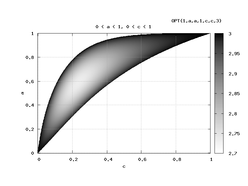
Figure 1: OPT$(1,a,a,1,c,c,s)$ over the rectangle $0\leq a\leq 1,0\leq c\leq 1$ for $s=3$ and $s=14$.

Lemma 17

Let $s\geq 8,A(x)\,=\,A(x,s):=\,(7/10)Q\cdot x.$
(a) OPT$(y)\,\,:=$ OPT $\left(1,A(y),\,A(y),\,1,y,\,y,\,s\right)$ is strictly decreasing for $0\leq y\leq 1/(2Q).$ The start value is OPT$(0)=3.$
(b) Given $0\leq y\leq 1/(2Q),$ OPT$(z):=$ OPT$(1,A(y+z),\,A(y-z),\,1,y+z,\,y-z,\,s)$ is decreasing in $0\leq z\leq y.$

Lemma 18

Let $s\,\geq 7\,\,$, and $\frac{7}{20}\leq A\leq 1-\frac{1}{Q}.$ Then
OPT$(z):=$ OPT$\left(1,A,\,A,\,1,1/(2Q)+z,\,1/(2Q)-z\,,\,s\right)\leq 3\,-\,\delta$ for $0\leq z\leq 1/(2Q).$

Lemma 19

Let $\,s\,\geq\,7,$ and $1/(2Q)\leq C\leq 1/2.$ Then
OPT$(z):=$ OPT$\left(1,1-1/Q,\,1-1/Q,\,1,C+z,\,C-z\,,s\right)\,\leq 3\,-\,\delta$ for $0\leq z\leq C.$

Lemma 20

Let $s\geq 15$ and $A(x)\,=\,A(x,s)\,:=\,1+7/(10Q)\cdot x\,-\,7/(10Q).$
(a) OPT$(y):=$OPT$\left(1,A(y),A(y),1,y,y,s\right)$ is strictly increasing in $4/10\leq y\leq 1.$ The final value is OPT$(1)=3.$
(b) Given $4/10\leq y\leq 1,$ OPT$(z):=$OPT$\left(1,A(y+z),A(y-z),1,y+z\,,y-z\,,\,s\right)$ is decreasing in $0\leq z\leq\min\{y,1-y\}.$

Proof of Theorem 9 from the preceding lemmas. We prove Theorem 9 for $\lambda_{0}\geq\lambda_{1}\geq\lambda_{2}>0$ first. We denote $P_{i}:=\lambda_{i}/\lambda_{0},\,\mbox{ then }1\geq P_{1}\geq P_{2}>0.$

Case 1: $P_{1}\,+\,P_{2}\leq\frac{7}{20Q}$. With $A(x)$ from Lemma 17 we have $A(x)\cdot x\,=\,(7/10)Q\cdot x^{2}.$ Thus there exist $y_{1}\geq y_{2}$ with $P_{i}=A(y_{i})\cdot y_{i}.$ We represent $y_{i}$ such that Lemma 17 is applicable.

$$y\,:=\,\frac{y_{1}+y_{2}}{2},\,\,z\,:=\,\frac{y_{1}-y_{2}}{2}.\mbox{ Then }y_{1}=y+z,y_{2}=y-z,0\leq z\leq y.$$

We show $y\leq\frac{1}{2Q}$ and Lemma 17 applies to $y,z.$

$$\frac{7}{20Q}\,\geq\,P_{1}+P_{2}\,=\,\frac{7}{10}Q(y_{1}^{2}+y_{2}^{2})\Longrightarrow y_{1}^{2}+y_{2}^{2}\,\leq\,\frac{1}{2Q^{2}}.$$

$$(y_{1}+y_{2})^{2}\leq 2y_{1}^{2}+2y_{2}^{2}\leq\frac{1}{Q^{2}}\mbox{ and }y=\frac{y_{1}+y_{2}}{2}\leq\frac{1}{2Q}.$$

With $a_{0}=c_{0}=1,a_{1}=A(y+z),a_{2}=A(y-z),c_{1}=y+z,c_{2}=y-z$ we have $a_{i}c_{i}=P_{i}.$ By Lemma 16 $\Psi:=\Psi(\bar{\omega},\bar{\lambda},\bar{a}\cdot s,\bar{c})\leq 1/3^{\gamma}\mbox{OPT},\,\,\mbox{OPT}:=\mbox{OPT}(\bar{a},\bar{c},s).$ If $P_{1}\geq\varepsilon$ for an $\varepsilon>0$ we have OPT$<3-\delta^{\prime}$ by Lemma 17 and Theorem 9 holds.

For smaller $P_{1}$ we have OPT $\leq 3,$ approaching $3$. Only (1) of Theorem 9 holds. To get (2) for small $P_{1}$ we argue as follows: For $P_{1}$ approaching $0$ we see that $c_{1}$ and $c_{2}$ approach $0.$ We consider the treatment of the factor $r(\bar{c})$ in the proof Lemma 16. Both $C_{1}$ and $C_{2}$ from this proof approach $1$ in this case. Therefore we have a $\delta^{\prime}>0$ such that $(C_{1}^{k}+2C_{2}^{k/2})^{\gamma}\leq C_{1}^{k\gamma}+2^{\gamma}C_{2}^{k\gamma/2}-\delta^{\prime}.$ As $a_{0}=c_{0}=1$ the first two factors of OPT do not approach $0.$ And we have $\Psi(\bar{\omega},\bar{\lambda},\bar{a}\cdot s,\bar{c})\leq(1/3^{\gamma})(\mbox{OPT}-\delta^{\prime\prime})\leq 3^{1-\gamma}-\delta$ and Theorem 9 (2) holds.

Case 2: $\frac{7}{20Q}\leq P_{1}\,+\,P_{2}\leq\left(1\,-\,\frac{1}{Q}\right)\frac{1}{Q}.$ To use Lemma 18 we define $A$ by $A\cdot\frac{1}{Q}=P_{1}+P_{2}.$ and $A$ is as required by Lemma 18. We need to find an appropriate $z.$ As $P_{1}\geq P_{2}$ there is a $y\geq\frac{1}{2}$ such that $P_{1}=A\frac{1}{Q}y$ and $P_{2}=A\frac{1}{Q}(1-y).$ With $y=\frac{1}{2}+z^{\prime}$ and $1-y=\frac{1}{2}-z^{\prime},z^{\prime}\leq\frac{1}{2},$ and $P_{1}=A\left(\frac{1}{2Q}+\frac{z^{\prime}}{Q}\right)\,,\,P_{2}\,=\,A\left(\frac{1}{2Q}-\frac{z^{\prime}}{Q}\right)$ Lemma 18 applies with $z=z^{\prime}/Q.$ Again we set $a_{0}=c_{0}=1$ and $a_{1}=a_{2}=A,c_{1}=\frac{1}{2Q}+z,c_{2}=\frac{1}{2Q}-z.$ By Lemma 16 $\Psi(\bar{\omega},\bar{\lambda},\bar{a}\cdot s,\bar{c})\leq 3^{1-\gamma}-\delta.$

Case 3: $\left(1\,-\,\frac{1}{Q}\right)\frac{1}{Q}\leq P_{1}+P_{2}\leq 1\,-\,\frac{1}{Q}.$ Let $C$ be given by $\left(1\,-\,\frac{1}{Q}\right)\cdot C\,=\,\frac{P_{1}+P_{2}}{2}.$ Then $C$ is as required by Lemma 19. We have a $0\leq z^{\prime}\leq\frac{1}{2}$ such that

$$P_{1}\,=\,\left(1\,-\,\frac{1}{Q}\right)\cdot C\cdot 2\left(\frac{1}{2}\,+\,z^{\prime}\right)\,\,=\left(1\,-\,\frac{1}{Q}\right)\cdot(C\,+\,2Cz^{\prime}),$$

$$P_{2}\,=\,\left(1\,-\,\frac{1}{Q}\right)\cdot(C-2Cz^{\prime}).$$

With $z=2Cz^{\prime}\leq C$ Lemma 19 applies. We set $a_{0}=c_{0}=1$ and $a_{1}=a_{2}=1-1/Q$ and $c_{1}=C+z,c_{2}=C-z$ and finish the argument as in Case 2.

Case 4: $P_{1}+P_{2}\geq 1-\frac{1}{Q}.$ With $A(x)$ as from Lemma 20 we have $A(x)\cdot x\,=\,\left(1-\frac{7}{10Q}\right)x\,+\,\frac{7}{10Q}x^{2}$ and $A(x)x$ increases from $0$ to $1$ for $0\leq x\leq 1.$ Let $y_{i}$ be such that $P_{i}\,=\,A(y_{i})\cdot y_{i}.$ Then $y_{2}\leq y_{1}\leq 1$ and we can represent $y_{i}$ such that Lemma 20 is applicable.

$$y:=\frac{y_{1}+y_{2}}{2},z:=\frac{y_{1}-y_{2}}{2},\mbox{ and }y_{1}=y+z,y_{2}=y-z,z\leq y,1-y.$$

We show that $1\geq y\geq 4/10$ and Lemma 20 applies to $y,z.$ We have $P_{1}+P_{2}=A(y_{1})y_{1}+A(y_{2})y_{2}=y_{1}+y_{2}+7/(10Q)(y_{1}^{2}+y_{2}^{2}-y_{1}-y_{2})\leq y_{1}+y_{2}.$ Therefore $y=(y_{1}+y_{2})/2\geq 1/2(1-1/Q)\geq 4/10$ as $Q\geq s\geq 15.$ Setting $a_{0}=c_{0}=1,a_{1}=A(y+z),a_{2}=A(y-z),c_{1}=y+z,c_{2}=y-z$ implies the claim.

Now, assume the $\lambda_{i}$ are ordered in a different way. We apply the permutation leading from $\lambda_{0}\geq\lambda_{1}\geq\lambda_{2}$ to the ordering considered to the $P_{i},a_{i},c_{i}$ above. The first two factors of $\Psi$ do not change, only $r(\bar{c})$ may change. But, Lemma 16 still applies. The three factors, OPT₁, OPT₂, OPT₃ of OPT$(\bar{a},\bar{c},s)$ do not change. This refers to $C_{1},$ and $C_{2},$ too, and the argument above for $P_{1}$ small applies, too. ∎

In the proofs to come in the following four subsections we use the notation

$$L(a,s)=\frac{q(as)}{q(s)}=\frac{\exp(as)-as-1}{\exp(s)-s-1},\,K(a,s)=\frac{q^{\prime}(as)}{q^{\prime}(s)}\,=\,\frac{\exp(as)-1}{\exp(s)-1},$$

$$M(a,s)=\frac{\exp(as)}{\exp(s)}.\mbox{Then }aK(a,s)\leq L(a,s)\leq K(a,s)\leq M(a,s)\,,\,0\leq a\leq 1.\,$$ (7)

Proof of (7.) $p(x):=q^{\prime}(x),\,K:=K(a,s),L:=L(a,s).$ For $a=0$ or $a=1$ we have $aK=L.$ For $a>0,$ $aK\leq L\Longleftrightarrow ap(as)/q(as)\leq p(s)/q(s)\Longleftrightarrow asp(as)/q(as)\leq sp(s)/q(s).$ The preceding inequality holds trivially for $a=1.$ We show that $asp(as)/q(as)$ is strictly increasing in $a>0.$ We observe that $q(x)/(xp(x))=1/x-1/p(x).$ The derivative is of the last expression is $<0$ iff $x^{2}+2<\exp(x)+1/\exp(x).$ For $x=0$ we have equality and several differentiations show the inequality.

For $a=0,L\leq K$ is true. For $a>0$ $L\leq K\Longleftrightarrow 1-sa/p(sa)\leq 1-s/p(s).$ The last inequality follows from $a\geq p(sa)/p(s)$ for $0\leq a\leq 1.$ This follows from convexity. $K(a,s)\leq M(a,s)$ is very easy to show. ∎

$$\mbox{We also have }aK(a,s)\leq\frac{7}{10}L(a,s),\,\mbox{ for }0\leq a\leq\frac{1}{2},s\geq 4\,\,\,\mbox{ (proof omitted.) }$$ (8)

$$\mbox{ We recall }Q(x)=\frac{xq^{\prime}(x)}{q(x)}=\frac{x(\exp(x)-1)}{\exp(x)-x-1},Q=Q(s)=k\gamma,\,Q(s)>s.$$

3.1 Proof of Lemma 17

Lemma 17 (repeated) Let $s\geq 8,A(x)\,=\,A(x,s):=\,(7/10)Q\cdot x.$
(a) OPT$(y)\,\,:=$ OPT $\left(1,A(y),\,A(y),1,\,y,\,y,s\right)$ is strictly decreasing for $0<y\leq 1/(2Q).$ The start value is OPT$(0)=3.$
(b) Given $0\leq y\leq 1/(2Q),$ OPT$(z):=$ OPT$(1,A(y+z),\,A(y-z),\,1,\,y+z,\,y-z,\,s)$ is decreasing in $0\leq z\leq y.$

Proof of (a). We have

$$\mbox{OPT}(y)=\left(1+2L(A(y),s)\right)\left(\frac{1}{1+2A(y)\cdot y}\right)^{Q}\left(\left(1\,+\,2y\right)^{Q}\,+\,2\left(1\,-\,y\right)^{Q}\right).$$

$$\mbox{ We write OPT}_{1}(y)\,=\,1+2L(A(y),s).\mbox{ Clearly OPT}(0)\,=\,3.$$

$$\mbox{ We have }A^{\prime}:=\frac{d}{dy}\,A(y)\,=\,\frac{7}{10}Q.\,\,\,\,\mbox{ And }\frac{d}{dy}\ln\mbox{ OPT }(y)\,>=<\,0\Longleftrightarrow$$

$$\frac{A^{\prime}\cdot 2\cdot K(A(y),s)\,}{\mbox{ OPT}_{1}(y)}\,-\,\frac{2A(y)\,+\,2A^{\prime}\cdot y}{1+2A(y)\cdot y}\,+\,\frac{2(1+2y)^{Q-1}-2(1-y)^{Q-1}}{\left(1\,+\,2y\right)^{Q}\,+\,2\left(1\,-\,y\right)^{Q}}$$

$$\,>=<\,0$$ (9)

The relationship (9) is obtained by taking the derivative and dividing by $Q.$ To get the first summand we look into the definition of $Q$ (the formula after 8.)

$$\frac{d}{dy}\ln\mbox{ OPT }_{1}(y)=\frac{\frac{A^{\prime}s\cdot 2(\exp(A(y)s)-1)}{q(s)}}{\mbox{ OPT}_{1}(y)}\,,\,\frac{1}{Q(s)}\frac{A^{\prime}s\cdot 2(\exp(A(y)s)-1)}{q(s)}=A^{\prime}\cdot 2K(A(y),s)$$

Observe that the first and third term of (9) is $\geq 0$ for $0\leq y\leq 1$ whereas the second term is $\leq 0.$ Moreover, $A^{\prime}\cdot y=A(y).$ We have that $\frac{d}{dy}\ln\mbox{ OPT }(y)\,<\,0$ if the following two inequalities both hold:

$$\frac{A^{\prime}\cdot 2\cdot K(A(y),s)}{\mbox{ OPT}_{1}(y)}\,<\,\frac{\,\frac{7}{10}A^{\prime}\cdot y}{1+2A(y)\cdot y}$$ (10)

$$\frac{2(1+2y)^{Q-1}-2(1-y)^{Q-1}}{\left(1\,+\,2y\right)^{Q}\,+\,2\left(1\,-\,y\right)^{Q}}\,<\frac{\frac{33}{10}A^{\prime}\cdot y}{1+2A(y)\cdot y}\,\,$$ (11)

Note that for $y=0$ both sides of the first inequality are equal to $0$ and of the second inequality, too. The derivative of OPT$(y)$ is $=0$ for $y=0.$

Comment: It is important to split up the left-hand-side of inequality (9), otherwise the calculations get very complicated. Equally important is the step leading to (9). Analogous steps will occur several times.

Proof of (10) for $0<y\leq 1/(2Q)\,\,,\,\,s\geq 7$ . We abbreviate $K:=K(A(y),s)\,\,,L:=L(A(y),s).$ Note OPT${}_{1}(y)\,=\,1+2L.$ As $A^{\prime}>0$ we show

$$\frac{2\cdot K}{1+2L}\,<\,\frac{\frac{7}{10}y}{1+2A(y)\cdot y}\Longleftrightarrow 2K+4K\cdot A(y)\cdot y-2\frac{7}{10}L\cdot y\,<\,\frac{7}{10}y.$$

$$\mbox{ By (\ref{BAKL7/10}) we know }K\cdot A(y)\leq\frac{7}{10}L\mbox{ for }s\geq 4\mbox{ as}A(y)\leq\frac{1}{2}\mbox{ ( by }y\leq\frac{1}{2Q}.)$$ (12)

Thus (10) follows from $2K+2K\cdot A(y)\cdot y<\frac{7}{10}y.$ As $2K\cdot A(y)\cdot y\,\leq\,2K$ and $2K$ is convex and $2K=0$ for $y=0$ we show that $2K<(7/20)y$ for $y=1/(2Q).$ For $y=1/(2Q)$ we have $A(y)=7/20$ and $2K=2(\exp((7/20)s)-1)/(\exp(s)-1).$ As $1/(2Q)=(\exp(s)-s-1)/(2s(\exp(s)-1))$ we have for $y=1/(2Q)$

$$2K\,<\,\frac{7}{20}y\Longleftrightarrow 2\left(\exp\left(\frac{7}{20}s\right)-1\right)\,<\,\frac{7}{40}\frac{\exp(s)-s-1}{s}$$

This last inequality holds for $s\geq 7$ (but not for $s\leq 4.$ )

Proof of (11) for $y\leq 1/Q$ and $s\geq 2.$ Inequality (11) is equivalent to

$$2(1+2y)^{Q-1}-2(1-y)^{Q-1}\,<\,$$

$$<A(y)\left[\frac{33}{10}\left[\left(1\,+\,2y\right)^{Q}\,+\,2\left(1\,-\,y\right)^{Q}\right]\,-\,2y\cdot\left[2(1+2y)^{Q-1}-2(1-y)^{Q-1}\right]\right]\,\,$$ (13)

$$\mbox{ The right-hand-side of (\ref{klsymugl210}) is }\,\geq\,$$

$$A(y)\left[\frac{33}{10}\left[\left(1\,+\,2y\right)^{Q}\,+\,2\left(1\,-\,y\right)^{Q}\right]\,-\,\frac{33}{10}y\cdot\left[2(1+2y)^{Q-1}-2(1-y)^{Q-1}\right]\right]$$

$$=\,\frac{33}{10}A(y)\left[\left(1\,+\,2y\right)^{Q-1}(1+2y-2y)\,+\,2\left(1\,-\,y\right)^{Q-1}(1-y+y)\right]$$

$$=\,\frac{33}{10}A(y)\left[\left(1\,+\,2y\right)^{Q-1}\,+\,2\left(1\,-\,y\right)^{Q-1}\right].$$

$$\mbox{ And (\ref{klsymugl210}) follows from }\frac{2(1+2y)^{Q-1}-2(1-y)^{Q-1}}{(1+2y)^{Q-1}+2(1-y)^{Q-1}}\,<\,\frac{33}{10}A(y)$$ (14)

For $y=0$ both sides of (14) are equal to $0.$ We show that $33/10\cdot A^{\prime}\,>\,$ the derivative with respect to $y$ of the left-hand-side of (14.) By elementary calculation

$$\frac{d}{dy}\frac{2(1+2y)^{Q-1}-2(1-y)^{Q-1}}{(1+2y)^{Q-1}+2(1-y)^{Q-1}}\,=\,\frac{18\cdot(Q-1)(1+y-2y^{2})^{Q-2}}{\left[(1+2y)^{Q-1}+2(1-y)^{Q-1}\right]^{2}}.$$

$$\mbox{ We need to show }\frac{33}{10}\frac{7}{10}Q\left[(1+2y)^{Q-1}+2(1-y)^{Q-1}\right]^{2}\,>\,18(Q-1)(1+y-2y^{2})^{Q-2}.$$

$$\mbox{ Enlarging the right-hand-side, }1\leq 1+y-2y^{2}\mbox{ for }y\leq 1/Q\leq 1/s\leq 1/2\mbox{(by }Q(s)\geq s)$$

$$\mbox{ we show }33\cdot 7\left[(1+2y)^{Q-1}+2(1-y)^{Q-1}\right]^{2}\,>\,1800(1+y-2y^{2})^{Q-1}\,$$

$$=\,1800\left((1+2y)(1-y)\right)^{Q-1}$$

$$\Longleftrightarrow 231\left[(1+2y)^{2(Q-1)}\,+\,4\left((1+2y)(1-y)\right)^{Q-1}\,+\,4(1-y)^{2(Q-1)}\right]\,>$$

$$>\,1800\left((1+2y)(1-y)\right)^{Q-1}\Longleftrightarrow\mbox{ (Division by }\left((1+2y)(1-y)\right)^{Q-1}\mbox{)}$$

$$\Longleftrightarrow\,\,\left(\frac{1+2y}{1-y}\right)^{Q-1}\,+\,4\,+\,\,4\left(\frac{1-y}{1+2y}\right)^{Q-1}\,>\,1800/231.$$

$$\mbox{ Rescaling the fraction to }x\mbox{ the preceding inequality follows from }$$

$$x+4\frac{1}{x}>1800/231-4\,=3.79\dots\,\mbox{ true for }\,x>0.$$

Proof of (b). We assume $0\leq y\leq 1/(2Q)$ and $0<z\leq y.$

$$A(y+z)=\frac{7}{10}Q\cdot(y+z)\,\,\,\,,\,A(y+z)\cdot(y+z)\,=\,\frac{7}{10}Q\cdot(y+z)^{2}$$

$$A(y+z)\cdot(y+z)\,+\,A(y-z)\cdot(y-z)\,=\,\frac{7}{10}Q\cdot 2(y^{2}+z^{2})$$

$$\mbox{OPT}(z)\,=\,\left(1\,+\,L(A(y+z),s)\,+\,L(A(y-z),s)\right)\cdot$$

$$\cdot\left(\frac{1}{1+\frac{7}{10}Q\cdot 2(y^{2}+z^{2})}\right)^{Q}\cdot\left((1+2y)^{Q}\,+\,2\cdot\left((1-y)^{2}\,+\,3z^{2}\right)^{Q/2}\right).$$

$$\frac{d}{dz}\ln\mbox{OPT}(z)\,>=<\,0\Longleftrightarrow$$

$$\frac{\frac{7}{10}Q\cdot K(A(y+z),s)\,-\,\frac{7}{10}Q\cdot K(A(y-z),s)}{1\,+\,L(A(y+z),s)\,+\,L(A(y-z),s)\,}\,\,-\,\,\frac{\frac{7}{10}Q4z}{1+\frac{7}{10}Q\cdot 2(y^{2}+z^{2})}\,+\,$$

$$\frac{6z\cdot((1-y)^{2}+3z^{2})^{Q/2-1}}{(1+2y)^{Q}\,+\,2\cdot((1-y)^{2}+3z^{2})^{Q/2}}\,\,>=<\,\,0.$$

The first term of the sum is obtained as the first term of (9.) The first and third term of the left-hand-side of the preceding inequality are $\geq 0$ for $0\leq z\leq y$ whereas the second term is $\leq 0.$

Analogously to (10) and (11) $\frac{d}{dz}\ln\mbox{OPT}(z)\,<\,0$ is implied by

$$\frac{\frac{7}{10}Q\left[K(A(y+z),s)\,-\,K(A(y-z),s)\right]}{1\,+\,L(A(y+z),s)\,+\,L(A(y-z),s)}\,\,<\,\,\frac{\frac{9}{10}\frac{28}{10}Qz}{1+\frac{14}{10}Q(y^{2}+z^{2})}$$ (15)

$$\frac{6z\cdot((1-y)^{2}+3z^{2})^{Q/2-1}}{(1+2y)^{Q}\,+\,2\cdot((1-y)^{2}+3z^{2})^{Q/2}}\,<\,\frac{\frac{1}{10}\frac{28}{10}Qz}{1+\frac{14}{10}Q(y^{2}+z^{2})}$$ (16)

Proof of (15) for $y\leq 1/(2Q)$ and $s\geq 3.5.$ The denominator of the right-hand-side fraction is maximal for $y=z=1/(2Q).$ In this case it is $1+7/(10Q)<1+1/Q.$ We lower the denominator of the left-hand-side simply to $1.$ The claim follows from

$$K(A(y+z),s)\,-\,K(A(y-z),s)\,<\,\frac{\frac{18}{5}z}{1+\frac{1}{Q}}$$

The left-hand-side of the preceding inequality is convex in $z$ for all $y<1/(2Q)$ (based on the convexity of $\exp(x)-\exp(-x).$) For $z=0$ both sides are $=0.$ Therefore it is sufficient to show that the inequality holds for $z=y$ where $y\leq 1/(2Q).$ Setting $z=y$ yields $K(A(y-z),s)=0$ and we show

$$K(A(2y),s)\,\,<\,\frac{\frac{18}{5}y}{1+\frac{1}{Q}}$$

Again by convexity of the left-hand-side it is sufficient to show the inequality for $y=1/(2Q).$ In this case we need to show

$$K(A(1/Q),s)\,=\,\frac{\exp\left(\frac{7}{10}s\right)-1}{\exp(s)-1}\,<\,\frac{18}{10}\frac{1}{Q+1}$$

$$\mbox{ By (\ref{BAKL}) we know }\frac{\exp\left(\frac{7}{10}s\right)-1}{\exp(s)-1}\,\leq\,\exp\left(-\frac{3}{10}s\right).$$

$$\mbox{ And }\exp\left(-\frac{3}{10}s\right)\,<\,\frac{18}{10}\frac{1}{Q+1}\mbox{ holds (proof omitted) for }s\geq 3.5.$$

Proof of (16) for $s\geq 8.$ We show

$$\frac{(1+2y)^{Q}\,+\,2\cdot((1-y)^{2}+3z^{2})^{Q/2}}{6z\cdot((1-y)^{2}+3z^{2})^{Q/2-1}}\,>\,\frac{1+\frac{14}{10}Q(y^{2}+z^{2})}{\frac{1}{10}\frac{28}{10}Qz}.$$

$$\mbox{ Canceling }z\mbox{ in the denominator , setting }z=y\mbox{ on the right-hand-side, this follows from }$$

$$\frac{(1+2y)^{Q}}{6\cdot((1-y)^{2}+3z^{2})^{Q/2-1}}\,+\,\frac{1}{3}((1-y)^{2}+3z^{2})\,>\,\frac{1+\frac{14}{5}Qy^{2}}{\frac{28}{100}Q}\,=\,\frac{100}{28Q}+10y^{2}$$

$$\mbox{As }(1-y)^{2}+3z^{2}\,\leq\,1-2y+4y^{2}\,<1\mbox{ by }y\leq 1/(2Q),Q\geq s\geq 8$$

$$\mbox{ this follows from }\frac{1}{6}(1+2y)^{Q}\,+\,\frac{1}{3}(1-y)^{2}\,>\,\frac{100}{28Q}+10y^{2}$$

The last inequality holds for $Q\geq 8,y\geq 0$ and then the claim holds as $Q\geq s.$

3.2 Proof of Lemma 18

Lemma 18 (repeated) Let $s\,\geq 7\,\,$ and $\frac{7}{20}\leq A\leq 1-\frac{1}{Q}.$ Then
OPT$(z):=$ OPT$\left(1,A,\,A,\,1,1/(2Q)+z,\,1/(2Q)-z\,,s\right)\leq 3\,-\,\delta$ for $0\leq z\leq 1/(2Q).$

Proof

OPT$(z)\,=\,$

$$\left(1\,+\ 2\cdot L(A,s)\right)\left(\frac{1}{1+\frac{A}{Q}}\right)^{Q}\cdot\left[\left(1+\frac{1}{Q}\right)^{Q}\,+\,2\left(\left(1-\frac{1}{2Q}\right)^{2}+3z^{2}\right)^{1/2\cdot Q}\right]$$

is increasing in $z.$ We show the claim for $z=1/(2Q).$ Let from now on OPT$(A)\,=\,$ OPT$(1,A,A,1,1/Q,0,s)\,=\,$

$$\left(1\,+\ 2\cdot L(A,s)\right)\left(\frac{1}{1+\frac{A}{Q}}\right)^{Q}\cdot\left[\left(1+\frac{1}{Q}\right)^{Q}\,+\,2\left(1-\frac{1}{Q}+\frac{1}{Q^{2}}\right)^{1/2\cdot Q}\right]$$

First, we show that OPT$(A)$ has exactly one extremum in $0\leq A\leq 1$ which is a minimum.

$$\frac{d}{dA}\ln\mbox{OPT}(A)\,>=<\,0\Longleftrightarrow\frac{2K(A,s)}{1+2L(A,s)}\,-\,\frac{\frac{1}{Q}}{1+\frac{A}{Q}}\,>=<\,0.\,$$

Concerning the first term of the preceding sum we refer to the explanation following (9.) For $A=0$ the first term is $=0$ and the derivative is $<0.$ For $A=1$ the first term is $=2/3,$ whereas the second term is $1/(Q+1)\,<\,2/3$ for $Q>s>2,$ and the derivative is $>0.$ We show that the derivative is $=0$ for exactly one $0<A<1$ which must be a minimum.

The second fraction of the derivative is decreasing in $A.$ We check that the first fraction is increasing. Abbreviating $L=L(A,s),\,L^{\prime}\,=\,\frac{d}{dA}L(A,s)$ and analogously for $K,$ we get

$$\frac{d}{dA}\frac{2K(A,s)}{1+2L(A,s)}\,>\,0\Longleftrightarrow 2K^{\prime}(1+2L)\,>\,2K2L^{\prime}\Longleftrightarrow$$

$$\mbox{ (Multiplication with }(\exp(s)-s-1)(\exp(s)-1),\mbox{division by }2\mbox{ and }s\mbox{.)}$$

$$(\exp(s)-s-1)\exp(sA)\,+\,\exp(sA)2(\exp(sA)-sA-1)\,>\,2(\exp(sA)-1)^{2}$$

$$\Longleftrightarrow(\exp(s)-s-2sA)\exp(sA)\,>\,-\exp(sA)\,+\,2$$

$$\Longleftrightarrow\exp(s)-s-2sA\,>\,-1+2/\exp(sA)$$

$$\mbox{ which is true for }s>2,0<A<1\mbox{ by convexity of }2/\exp(sA).$$

We need to show the claim for the boundary values $A=7/20\,$ and $A=1-1/Q.$ First, $A=7/20:$

$$1\,+\,2L(A,s)\,\leq 1+2M(A,s)\,=\,1\,+\,2\exp(-13/20\cdot s)\,\,\,\mbox{ (by (\ref{BAKL}).)}$$

With the derivative of the logarithm and the Mean Value Theorem we can show that

$$\left(\frac{1+\frac{1}{Q}}{1+\frac{A}{Q}}\right)^{Q}\mbox{ is increasing in }Q\mbox{ towards its limit }\exp(13/20).\,\frac{2\left(1-\frac{1}{Q}\,+\,\frac{1}{Q^{2}}\right)^{1/2\cdot Q}}{\left(1+\frac{A}{Q}\right)^{Q}}$$

$$\mbox{ is decreasing in }Q=Q(s)\geq 2\mbox{ (proof by standard calculus methods) and therefore }$$

$$\mbox{ also in }s\mbox{ towards its limit }2\exp(-17/20).\mbox{ For }Q=7\mbox{ we get a value }\leq 0.9$$

$$\mbox{ Therefore, for all }\geq s\,\geq 7\mbox{( as }Q(s)\geq s)$$

$$\mbox{OPT}(A)\,<\,(1+\,2\exp(-13/20\cdot 7))(\exp(13/20)+0.9)\,=\,2.87\dots\,\,.$$

Now, $A=1-1/Q:$

$$1\,+\,2L(A,s)\,\leq\,1\,+\,2M(A,s)\,=\,1\,+\,2\exp\left(-\frac{s}{Q}\right)$$

$$\,=\,1+2\exp\left(-\frac{\exp(s)-s-1}{\exp(s)-1}\right)\mbox{decreasing in }s\mbox{ to }1+2\exp(-1).$$

$$\mbox{ For }s=7\mbox{ we get }\,1+2L(A,s)\leq 1.7404\dots$$

$$\left(\frac{1+\frac{1}{Q}}{1+\frac{A}{Q}}\right)^{Q}\,=\,\left(\frac{1+\frac{1}{Q}}{1\,+\,\frac{1}{Q}\,-\,\frac{1}{Q^{2}}}\right)^{Q}\mbox{ is decreasing in }Q=Q(s)$$

$$\mbox{ (elementary proof omitted) and therefore in}\,\,s\mbox{ to }1.$$

$$\mbox{ For }Q=7\mbox{ we get }1.1344\dots.\mbox{ As }Q(s)\geq s\,\mbox{this bound applies to }s=7\mbox{, too.}$$

$$\frac{2\left(1-\frac{1}{Q}+\frac{1}{Q^{2}}\right)^{1/2\cdot Q}}{\left(1+\frac{1}{Q}-\frac{1}{Q^{2}}\right)^{Q}}\mbox{is again decreasing (proof omitted) in }$$

$$Q\mbox{ and }s\mbox{ to }2\exp(-3/2).\mbox{ For }Q=7\mbox{ we get }0.564\dots$$

$$\mbox{Altogether for }Q(s)\geq s\geq 7$$

$$\mbox{OPT}(A)\leq 1.741\cdot(1.135+0.565)\,=2.9597.$$

3.3 Proof of Lemma 19

Lemma 19 (repeated) Let $\,s\,\geq\,7$ and $1/(2Q)\leq C\leq 1/2.$ Then
OPT$(z):=$ OPT$\left(1,1-1/Q,\,1-1/Q,\,1,C+z,\,C-z\,,s\right)\,\leq 3\,-\,\delta$ for $0\leq z\leq C.$

Proof

We abbreviate $A=1-1/Q.$ First, analogously to the proof of Lemma 18 we can restrict attention to $z=C.$ OPT$(z)\,=\,$

$$=\,\left(1+2L(A,s)\right)\left(\frac{1}{1+2AC}\right)^{Q}\left[(1+2C)^{Q}\,+\,2((1-C)^{2}+3z^{2})^{1/2\cdot Q}\right]$$

$$\mbox{ Let from now on OPT}(C)\,=\,\mbox{OPT}(1,A,A,1,2C,0,s)\,=\,$$

$$=\,\left(1+2L(A,s)\right)\left(\frac{1}{1+2AC}\right)^{Q}\cdot\left[(1+2C)^{Q}\,+\,2(1+4C^{2}-2C)^{1/2\cdot Q}\right]$$

OPT$(C)$ has exactly one extremum, which is a minimum for $0\leq C\leq 1.$

$$\frac{d}{dc}\ln\mbox{OPT}(C)\,>=<\,0\Longleftrightarrow$$

$$-\frac{2A}{1+2AC}\,+\,\frac{2(1+2C)^{Q-1}\,+\,(8C-2)(1+4C^{2}-2C)^{1/2\cdot Q-1}}{(1+2C)^{Q}\,+\,2(1+4C^{2}-2C)^{1/2\cdot Q}}\,>=<\,0\Longleftrightarrow$$

$$2A\left((1+2C)^{Q}\,+\,2(1+4C^{2}-2C)^{1/2Q}\right)\,-$$

$$-\,2AC\left(2(1+2C)^{Q-1}\,+\,(8C-2)(1+4C^{2}-2C)^{1/2\cdot Q-1}\right)\,=$$

$$\,=\,2A\left[(1+2C)^{Q-1}\,+\,(2-2C)(1+4C^{2}-2C)^{1/2\cdot Q-1}\right]\,<\,\,=\,\,>$$

$$\,<\,\,=\,\,>\,2(1+2C)^{Q-1}\,+\,(8C-2)(1+4C^{2}-2C)^{1/2\cdot Q-1}\Longleftrightarrow$$

$$2A\,<\,\,=\,\,>\,\frac{2(1+2C)^{Q-1}\,+\,(8C-2)(1+4C^{2}-2C)^{1/2\cdot Q-1}}{(1+2C)^{Q-1}\,+(2-2C)(1+4C^{2}-2C)^{1/2\cdot Q-1}}\,\Longleftrightarrow\,$$

$$A\,<\,\,=\,\,>\,\frac{(1+2C)^{Q-1}\,+\,(4C-1)(1+4C^{2}-2C)^{1/2\cdot Q-1}}{(1+2C)^{Q-1}\,+(2-2C)(1+4C^{2}-2C)^{1/2\cdot Q-1}}$$

For $C=0$ the right-hand-side fraction is equal to $0<A$ and OPT$(C)$ is decreasing. For $C=1$ the right-hand-side fraction is greater than $1>A$ and OPT$(C)$ is increasing.

Next we show that the preceding fraction is increasing in $0<C<1,$ and equality is attained for only one $C$ which must be a minimum.

$$\mbox{ Rewriting }4C-1\,=\,(2-2C)+6C-3\mbox{ the fraction is rewritten as }$$

$$1\,+\,\frac{(6C-3)(1+4C^{2}-2C)^{1/2\cdot Q-1}}{(1+2C)^{Q-1}\,+(2-2C)(1+4C^{2}-2C)^{1/2\cdot Q-1}}$$

$$\mbox{ Rescaling }1/2\cdot Q-1\mbox{ to }Q\mbox{ ( then }Q-1\mbox{ scales to }2Q+1)\mbox{ and }2C\mbox{ to }C\mbox{ we get }$$

$$1\,+\,\frac{(3C-3)(1+C^{2}-C)^{Q}}{(1+C)^{2Q+1}\,+(2-C)(1+C^{2}-C)^{Q}}\,\,$$

$$\mbox{ Dividing through }3(C-1)(1+C^{2}-C)^{Q}\mbox{ the preceding fraction is certainly increasing if }$$

$$\frac{(1+C)^{2Q+1}}{3(C-1)(1+C^{2}-C)^{Q}}\mbox{ and }\frac{2-C}{3(C-1)}\mbox{ are both decreasing for }0<C<2,C\neq 1.$$

The second fraction is easily seen to be decreasing. We show that the inverse of the first fraction is increasing. The numerator of its derivative is

$$\left[(1+C^{2}-C)^{Q}\,+\,(C-1)(2C-1)Q(1+C^{2}-C)^{Q-1}\right]\cdot(1+C)^{2Q+1}\,\,-\,$$

$$-\,(C-1)(1+C^{2}-C)^{Q}\cdot(2Q+1)(1+C)^{2Q}\,\,\,=\,(1+C)^{2Q}(1+C^{2}-C)^{Q-1}\cdot$$

$$\left[(1+C)(1+C^{2}-C)\,+\,(1+C)(C-1)(2C-1)Q\,-\,(2Q+1)(C-1)(1+C^{2}-C)\right]$$

The expression in square brackets can be rewritten as

$$(1+C)(C-1)(2C-1)Q\,-\,2Q(C-1)(1+C^{2}-C)\,+\,(-C+1+C+1)(1+C^{2}-C)$$

$$=\,\,Q(1-C)^{2}\,+\,2(1+C^{2}-C)\,>\,0$$

Now it is sufficient to show the claim for the boundary values, $C=1/(2Q)$ and $C=1/2.$ The first case is contained in Lemma 18. Let $C=1/2.$ We proceed as in the proof of Lemma 18, case $A=1-1/Q.$

$$1+2L(A,s)\leq 1.7404\mbox{ for }s\geq 7$$

$$\left(\frac{1+2C}{1\,+\,2CA}\right)^{Q}\,=\,\left(\frac{2}{2\,-\,\frac{1}{Q}}\right)^{Q}\mbox{ is decreasing in }Q=Q(s)$$

$$\mbox{ (elementary proof omitted) and therefore in}\,\,s\mbox{ to }\exp(-1/2).$$

$$\mbox{ For }Q=7\mbox{ we get }1.67993\dots.\mbox{ As }Q(s)\geq s\,\mbox{this bound applies to }s=7\mbox{, too.}$$

$$\frac{2(1+4C^{2}-2C)^{1/2\cdot Q}}{(1+2AC)^{Q}}\,=\,\frac{2}{(2-\frac{1}{Q})^{Q}}\mbox{ decreasing to }0$$

$$\mbox{ For }Q=7\mbox{ we get }0.02624\dots$$

$$\mbox{ Altogether OPT}(C)\leq 1.75\cdot(1.68+0.027)=2.98\mbox{ for }s\geq 7.$$

3.4 Proof of Lemma 20

Lemma 20 (repeated) Let $s\geq 15$ and $A(x)\,=\,A(x,s)\,:=\,1+7/(10Q)\cdot x\,-\,7/(10Q).$
(a) OPT$(y):=$OPT$\left(1,A(y),A(y),1,y,y,s\right)$ is strictly increasing in $4/10\leq y<1.$ The final value is OPT$(1)=3.$
(b) Given $4/10\leq y\leq 1,$ OPT$(z):=$OPT$\left(1,A(y+z),A(y-z),1,y+z,y-z,s\right)$ is decreasing in $0\leq z\leq\min\{y,1-y\}.$

Proof of (a). We have OPT$(y)\,=\,$

$$\left(1+2L(A(y),s)\right)\left(\frac{1}{1+2A(y)\cdot y}\right)^{Q}\left(\left(1\,+\,2y\right)^{Q}\,+\,2\left(1\,-\,y\right)^{Q}\right)$$

$$\mbox{ We write OPT}_{1}(y)=1+2L(A(y),s).\mbox{ Clearly OPT}(1)\,=\,3$$

$$\mbox{ We have }A^{\prime}:=\frac{d}{dy}\,A(y)\,=\,\frac{7}{10}\frac{1}{Q}.$$

$$\frac{d}{dy}\ln\mbox{ OPT }(y)\,>=<\,0\Longleftrightarrow\mbox{(See comment to (\ref{EQKEY}.))}$$

$$\frac{A^{\prime}\cdot 2\cdot K(A(y),s)}{\mbox{ OPT}_{1}(y)}\,-\,\frac{2A(y)\,+\,2A^{\prime}\cdot y}{1+2A(y)\cdot y}\,+\,\frac{2(1+2y)^{Q-1}-2(1-y)^{Q-1}}{\left(1\,+\,2y\right)^{Q}\,+\,2\left(1\,-\,y\right)^{Q}}\,>=<\,0$$

Observe that the first and third term of the preceding sum are $\geq 0$ for $0\leq y\leq 1$ whereas the second term is $\leq 0.$

We have that $\frac{d}{dy}\ln\mbox{ OPT }(y)>0$ if the following two inequalities both hold:

$$\frac{A^{\prime}\cdot 2\cdot K(A(y),s)}{\mbox{ OPT}_{1}(y)}\,>\,\frac{\,2A^{\prime}\cdot y}{1+2A(y)\cdot y}$$ (17)

$$\frac{2(1+2y)^{Q-1}-2(1-y)^{Q-1}}{\left(1\,+\,2y\right)^{Q}\,+\,2\left(1\,-\,y\right)^{Q}}\,>\frac{2A(y)}{1+2A(y)\cdot y}\,\,$$ (18)

Note that for $y=1$ both sides of the first inequality are equal to $7/(10Q)\cdot 2/3$ and of the second inequality $2/3.$ Therefore the derivative of OPT$(y)$ is $=0$ for $y=1.$

Proof of (17) for $1>y\geq\ 0\,\,,\,\,\,s\geq 4$ . Let $K=K(A(y),s)$ and $L=L(A(y),s).$

$$\mbox{ As }A^{\prime}>0\mbox{ we need to show }\frac{K}{1+2L}\,>\,\frac{y}{1+2A(y)\cdot y}.$$

$$\Longleftrightarrow K\,+\,2K\cdot A(y)y\,-\,2L\cdot y\,>\,y$$

$$\mbox{ As }K\geq L\,\,\mbox{ by (\ref{BAKL}) this follows from }$$

$$K\left(1\,+\,2A(y)\cdot y\,-2y\right)\,\,=\,K\left(1+2\frac{7}{10Q}y^{2}-2\frac{7}{10Q}y)\right)\,>\,y$$ (19)

For $y=1$ both sides of (19) are $=1.$ For $y=0$ (19) holds as $K>0$ in this case.

$K$ considered as a function in $y$ is convex, increasing and $>0.$ The second term on the left-hand-side of (19), $1-2\frac{7}{10Q}y^{2}+2\frac{7}{10Q}y,$ is convex, $>0,$ and increasing for $y>1/2.$ Therefore the left-hand-side of (19) is convex for $1/2<y<1.$ We next show that the derivative of the left-hand-side at $y=1$ is $<1.$ This implies that (19) holds for $1/2\leq y<1.$

$$\frac{d}{dy}K\left(1\,+\,2\frac{7}{10Q}y^{2}\,-\,2\frac{7}{10Q}y)\right)\,=\,\frac{s\cdot\frac{7}{10Q}\cdot\exp(sA(y))}{\exp(s)-1}$$

$$\cdot\left(1\,\,\,+2\frac{7}{10Q}y^{2}\,-\,2\frac{7}{10Q}y\right)\,+\,\frac{\exp(sA(y))-1}{\exp(s)-1}\cdot\left(4\frac{7}{10Q}y\,-\,2\frac{7}{10Q}\right).$$

$$\mbox{ Plugging in }\,\,y=1\,\,\mbox{ yields }\frac{7}{10Q}\left(\frac{s\exp(s)}{\exp(s)-1}+2\right)$$ (20)

For $s=4$ (20) is $0.9837\dots<1.$ As (20) is in decreasing in $s$ (proof omitted) (19) holds for all $s\geq 4$ and $1/2\leq y<1.$

$1-2\frac{7}{10Q}y^{2}+2\frac{7}{10Q}y$ is decreasing for $y<1/2.$ Therefore, for $0\leq y\leq 1/2,$ we can bound the left-hand-side of (19) from below by

$$K\left[\left(1+2\frac{7}{10Q}y^{2}-2\frac{7}{10Q}y\right)_{y=1/2}\right]$$

This function (the argument $y$ occurs only in $K$) is convex in $y$ . For $y=1/2$ it is $>y$ by the previous argument. For $y=1$ it is $<y.$ Therefore it is $>y$ for $0\leq y\leq 1/2.$ The claim is shown.

Proof of (18) for $y\geq 4/10$ and $s\geq 3.5.$ Inequality (18) is equivalent to

$$2(1+2y)^{Q-1}-2(1-y)^{Q-1}\,>\,$$

$$>2A(y)\left[\left(1\,+\,2y\right)^{Q}\,+\,2\left(1\,-\,y\right)^{Q}\,-\,y\cdot\left[2(1+2y)^{Q-1}-2(1-y)^{Q-1}\right]\right]\,=\,$$

$$=\,2A(y)\left[(1+2y)^{Q-1}(1+2y-2y)\,+\,2(1-y)^{Q-1}(1-y+y)\right)$$

$$\,=\,2A(y)\left[(1+2y)^{Q-1}+2(1-y)^{Q-1}\right]\Longleftrightarrow\frac{(1+2y)^{Q-1}-(1-y)^{Q-1}}{(1+2y)^{Q-1}+2(1-y)^{Q-1}}\,>\,A(y)$$ (21)

For $y=1$ both sides of (21) are equal to $1.$ For $y<1$ (21) can be rewritten as

$$\left(\frac{1+2y}{1-y}\right)^{Q-1}\,>\,\frac{2A(y)+1}{1-A(y)}.\mbox{ With }y=\frac{4}{10}\mbox{ this becomes }3^{Q-1}\,>\,\frac{30}{7}Q\,-\,2.$$

The preceding inequality holds for $Q>s\geq 3.5.$ and we have the claim for $y=4/10.$

To show the claim for $4/10<y<1$ we show that the left-hand-side of (21) is concave in $y.$ The derivative of the left-hand-side is

$$9(Q-1)\frac{(1+y-2y^{2})^{Q-2}}{\left[(1+2y)^{Q-1}\,+\,2(1-y)^{Q-1}\right]^{2}}$$

This is a decreasing function in $y\geq 4/10$ because the numerator is decreasing in this case whereas the denominator is increasing and $>0.$

Proof of (b). Some preparatory calculations:

$$A(y+z)\,=\,A(y)\,+\,\frac{7}{10Q}z\,\,,\,\,\,\,A(y-z)\,=\,A(y)\,-\,\frac{7}{10Q}z\,\,\,$$

$$A(y+z)\cdot(y+z)\,=\,A(y)y+A(y)z+\frac{7}{10Q}zy+\frac{7}{10Q}z^{2}$$

$$A(y-z)\cdot(y-z)\,=\,A(y)y-A(y)z-\frac{7}{10Q}zy+\frac{7}{10Q}z^{2}$$

$$A(y+z)\cdot(y+z)\,+\,A(y-z)\cdot(y-z)\,\,=\,2A(y)\cdot y+\frac{14}{10Q}z^{2}$$

We denote

$$\mbox{OPT}_{1}(z)\,=\,1\,+\,L(A(y+z),s)\,+\,L(A(y-z),s)$$

$$\mbox{Then OPT}(z)\,=\,\mbox{OPT}_{1}(z)\cdot\hfill$$

$$\cdot\left(\frac{1}{1+2A(y)\cdot y+\frac{14}{10Q}z^{2}}\right)^{Q}\cdot\left((1+y)^{Q}\,+\,2\cdot\left((1-y)^{2}\,+\,3z^{2}\right)^{Q/2}\right).$$

We proceed to show that $\frac{d}{dz}\ln$ OPT$(z)\,<\,0$ for $z>0.$ Some derivatives first.

$$\frac{d}{dz}\,A(y+z)\,=\,\frac{7}{10}\frac{1}{Q},\,\mbox{\quad\quad}\frac{d}{dz}\,A(y-z)\,=\,-\,\frac{7}{10}\frac{1}{Q},\,$$

$$\frac{d}{dz}\left(1+2A(y)\cdot y+\frac{14}{10Q}z^{2}\right)\,\,=\,\frac{28}{10Q}z\,$$

$$\frac{d}{dz}\left((1+y)^{Q}\,+\,2\cdot((1-y)^{2}+3z^{2})^{Q/2}\right)\,=\,6z\cdot Q\cdot((1-y)^{2}+3z^{2})^{Q/2-1}.$$

$$\frac{d}{dz}\ln\mbox{OPT}(z)\,>=<\,0\Longleftrightarrow\mbox{ (Recall comment to (\ref{EQKEY}).)}$$

$$\frac{\frac{7}{10Q}K(A(y+z),s)\,-\frac{7}{10Q}K(A(y-z),s)}{\mbox{OPT}_{1}(z)}\,\,-\,\,\frac{\frac{28}{10Q}z}{1+2yA(y)+\frac{14}{10Q}z^{2}}\,+\,$$

$$\frac{6z\cdot((1-y)^{2}+3z^{2})^{Q/2-1}}{(1+y)^{Q}\,+\,2\cdot((1-y)^{2}+3z^{2})^{Q/2}}\,\,>=<\,\,0.$$

Observe that the first and third term of the preceding inequality are $\geq 0$ for $0\leq z\leq\min\{y,1-y\},$ whereas the second term is $\leq 0.$

We have that $\frac{d}{dz}\ln\mbox{ OPT }(z)<0$ if the following two inequalities both hold:

$$\frac{\frac{7}{10Q}\left(K(A(y+z),s)\,-\,K(A(y-z),s)\right)}{\mbox{OPT}_{1}(z)}\,\,<\,\,\frac{\frac{11}{10Q}z}{1+2yA(y)+\frac{14}{10Q}z^{2}}$$ (22)

$$\frac{6z\cdot((1-y)^{2}+3z^{2})^{Q/2-1}}{(1+y)^{Q}\,+\,2\cdot((1-y)^{2}+3z^{2})^{Q/2}}\,<\,\frac{\frac{17}{10Q}z}{1+2yA(y)+\frac{14}{10Q}z^{2}}$$ (23)

Note that for $z=0$ both sides of the preceding inequalities are equal to $0$ and the derivative of $\ln\mbox{OPT}(z)$ is $=0.$ Moreover, we have $1+2yA(y)+\frac{14}{10Q}z^{2}\,\leq\,1+2y$ and the inequalities follow when they are shown with the denominator $1+2y$ in the right-hand-side fraction. To get this, observe that

$$2yA(y)+\frac{14}{10Q}z^{2}\,=\,2y+\frac{14}{10Q}\left(y^{2}-y+z^{2}\right)\leq 2y,$$

$$\mbox{as }z\leq\min\{y,1-y\}\mbox{ we have }z^{2}\leq y(1-y)\mbox{ or }y(y-1)+z^{2}\leq 0.$$

Proof of (22) for $0<z<\min\{y,1-y\},0\leq y\leq 1,s\geq 5$ . We enlarge the left-hand-side of (22) first:

$$K(A(y+z),s)\,-\,K(A(y-z),s)\,=\,\,\frac{1}{\exp(s)-1}\left(\exp(A(y+z)\cdot s)\,-\,\exp(A(y-z)\cdot s)\right)$$

$$=\,\,\frac{\exp(A(y)s)}{\exp(s)-1}\left[\exp\left(\frac{7}{10Q}sz\right)\,-\,\exp\left(-\,\frac{7}{10Q}sz\right)\right]$$

$$\mbox{OPT}_{1}(z)\,=\,1\,+\,L(A(y+z),s)\,+\,L(A(y-z),s)\,\,\,=\,1+\frac{1}{\exp(s)-s-1}\cdot$$

$$\cdot[\exp(A(y+z)s)\,-\,A(y+z)s\,-1\,+\,\exp(A(y-z)s)\,-\,A(y-z)s\,-1]$$

$$\geq\,\mbox{( As }A(y+z),A(y-z)\leq 1\mbox{.)}$$

$$1\,\,+\,\,\frac{1}{\exp(s)-1}[\exp(A(y+z)s)\,+\,\,\exp(A(y-z)s)\,-\,2s\,-2]\,\,=\,\frac{1}{\exp(s)-1}\cdot$$

$$\cdot\left[\exp(s)\,-2s\,-3\,+\,\exp(A(y)s)\left(\exp\left(\frac{7}{10Q}sz\right)\,+\,\exp\left(-\frac{7}{10Q}sz\right)\right)\right]$$

$$\geq\,\mbox{ (As }A(y)s\leq s\mbox{ and }s\geq 2\mbox{ so that }\exp(s)-2s-3>0\mbox{.)}$$

$$\frac{\exp(A(y)s)}{\exp(s)-1}\left[\frac{\exp(s)\,-2s\,-3}{\exp(s)}\,+\,\exp\left(\frac{7}{10Q}sz\right)\,+\,\exp\left(-\frac{7}{10Q}sz\right)\right]$$

$$\geq\,\frac{\exp(A(y)s)}{\exp(s)-1}\left[0.9\,+\,\exp\left(\frac{7}{10Q}sz\right)\,+\,\exp\left(-\frac{7}{10Q}sz\right)\right],$$

as $(\exp(s)-2s-3)/\exp(s)\geq 0.9$ for $s\geq 5.$ The denominator of the right-hand-side of (22) is enlarged by $1+2y\leq 3.$ We set

$$u=\exp\left(\frac{7}{10Q}sz\right)>1\mbox{ and show (simple algebra from (\ref{groasymugl1})) }\frac{u-\frac{1}{u}}{0.9+u+\frac{1}{u}}\,<\,\frac{11}{3\cdot 7}z$$

$$\mbox{ We have }z=(\ln u)\frac{10}{7}\frac{Q}{s}\,>\,(\ln u)\frac{10}{7}\mbox{ ( by }Q>s.)$$

$$\mbox{ Therefore it is enough to show }\frac{u-\frac{1}{u}}{0.9+u+\frac{1}{u}}\,<\,(\ln u)\frac{10}{7}\frac{11}{21}$$

$$\mbox{ Elementary means show that this is true for }u>1.$$

Proof of (23 ) for $s\geq 15,1\geq y\geq 2/10\,,\,0<z\leq\min\{y,1-y\}.$ Inequality (23) follows from

$$\frac{6z\cdot((1-y)^{2}+3z^{2})^{Q/2-1}}{(1+y)^{Q}}\,<\,\frac{\frac{17}{10Q}z}{1+2y}$$

$$\Longleftrightarrow 60Q(1+2y)((1-y)^{2}+3z^{2})^{Q/2-1}\,<\,17(1+y)^{Q}$$ (24)

For $y\leq 1/2$ we have $z\leq y$ and (24) follows from

$$60Q(1+2y)(1-2y+4y^{2})^{Q/2-1}\,<\,17(1+y)^{Q}$$

The preceding inequality holds for $Q\geq s\geq 15$ and $1/2\geq y\geq 2/10$ (proof omitted.)

For $y\geq 1/2$ we have $z\leq 1-y$ and (24) follows from

$$60Q(1+2y)(4(1-y)^{2})^{Q/2-1}\,<\,17(1+y)^{Q}$$

This inequality holds for $Q\geq s\geq 10$ and $y\geq 1/2$ (details omitted.)

4 Proof of Lemma 13 and Theorem 15

We consider $\Psi(\bar{\omega}\,,\,\bar{\lambda})\,=\,\Psi(\bar{\omega}\,,\,\bar{\lambda}\,,\,\bar{a}\,,\,\bar{c}\,)$ as function of $w_{i},\lambda_{i},$ $i=1,2$ in a neighborhood of $(\omega_{1},\omega_{2})=(\lambda_{1},\lambda_{2})=(1/3,1/3).$ The parameters $a_{i},c_{i}$ are given by $Q(a_{i})=\lambda_{i}k\gamma/\omega_{i},$ and $c_{0}=1,\,\,\,\,R(c_{1},c_{2})=(\lambda_{1}k,\lambda_{2}k).$ Subsection 5.1 shows that this is well defined and $a_{i},c_{i}$ is differentiable in $\lambda_{i},\omega_{i}.$ For $\lambda_{i}=1/3,\omega_{i}=1/3$ we have $a_{i}=s,c_{i}=1\,(Q(s)=k\gamma$ defining $s.$) We show that the partial derivatives of $\ln\Psi(\bar{\omega}\,,\,\bar{\lambda})$ are $0$ for $\omega_{i}=\lambda_{i}=1/3$ and the Hessian matrix is negative definite. This implies Lemma 13.

For $i=1,2$ the first derivatives are, with $a_{i}^{\prime},c_{i}^{\prime}$ denoting the right derivatives of $a_{i},c_{i}$ resp. and recalling that $Q(x)=\frac{xq^{\prime}(x)}{q(x)},q(x)=\exp(x)-x-1,R(x_{1},x_{2})=$
$\left(\frac{x_{1}r_{x_{1}}(1,x_{1},x_{2})}{r(1,x_{1},x_{2})}\,,\,\frac{x_{2}r_{x_{2}}(1,x_{1},x_{2})}{r(1,x_{1},x_{2})}\right)$

$$\frac{d\ln\Psi(\bar{\omega},\bar{\lambda})}{d\omega_{i}} = -\ln q(a_{0})+\omega_{0}\frac{a_{0}^{\prime}q^{\prime}(a_{0})}{q(a_{0})}+\ln\omega_{0}+1+$$ (25)

$$\quad+\ln q(a_{i})+\omega_{i}\frac{a_{i}^{\prime}q^{\prime}(a_{i})}{q(a_{i})}-\ln\omega_{i}-1-$$

$$\quad-k\gamma\lambda_{0}\frac{a_{0}^{\prime}}{a_{0}}-k\gamma\lambda_{i}\frac{a_{i}^{\prime}}{a_{i}}$$

$$= \ln\omega_{0}-\ln\omega_{i}+\ln q(a_{i})-\ln q(a_{0})\quad(\textrm{ using }Q(a_{i})=k\gamma\lambda_{i}/\omega_{i}).$$

$$\frac{d\ln\Psi(\bar{\omega},\bar{\lambda})}{d\lambda_{i}} = \omega_{0}\frac{a_{0}^{\prime}q^{\prime}(a_{0})}{q(a_{0})}+\omega_{i}\frac{a_{i}^{\prime}q^{\prime}(a_{i})}{q(a_{i})}+$$

$$\quad k\gamma\Bigg{(}-\ln\lambda_{0}-1+\ln a_{0}-\lambda_{0}\frac{a_{0}^{\prime}}{a_{0}}+$$

$$\quad\quad+\ln\lambda_{i}+1-\ln a_{i}-\lambda_{i}\frac{a_{i}^{\prime}}{a_{i}}-$$

$$\quad\quad-\ln c_{i}-\lambda_{1}\frac{c_{1}^{\prime}}{c_{1}}-\lambda_{2}\frac{c_{2}^{\prime}}{c_{2}}\Bigg{)}+$$

$$\quad\gamma\frac{c_{1}^{\prime}r_{c_{1}}(1,c_{1},c_{2})+c_{2}^{\prime}r_{c_{2}}(1,c_{1},c_{2})}{r(1,c_{1},c_{2})}$$

$$= k\gamma(\ln\lambda_{i}-\ln\lambda_{0}+\ln a_{0}-\ln a_{i}-\ln c_{i})$$

$$\quad(\mbox{ using }\,\,\,R(c_{1},c_{2})=(k\lambda_{1},k\lambda_{2}),Q(a_{i})=k\gamma\lambda_{i}/\omega_{i}))$$

For $\bar{\lambda}=\bar{\omega}=(1/3,1/3)$ the terms in (25) and (4) yield $0$.

The second derivatives (with $i,j\in\{1,2\},i\not=j)$ are (observe that some of the subsequent terms are equal as the derivative does not depend on the ordering of the variables)

$$\frac{d^{2}\ln\Psi(\bar{\omega},\bar{\lambda})}{d\lambda_{i},\lambda_{i}} = k\gamma\left(\frac{1}{\lambda_{i}}+\frac{1}{\lambda_{0}}+\frac{a_{0}^{\prime}}{a_{0}}-\frac{a_{i}^{\prime}}{a_{i}}-\frac{c_{i}^{\prime}}{c_{i}}\right)$$ (27)

$$\frac{d^{2}}{d\lambda_{i},\lambda_{j}} = k\gamma\left(\frac{1}{\lambda_{0}}+\frac{a_{0}^{\prime}}{a_{0}}-\frac{c_{i}^{\prime}}{c_{i}}\right)$$ (28)

$$\frac{d^{2}\ln\Psi(\bar{\omega},\bar{\lambda})}{d\omega_{i},\omega_{i}} = -\frac{1}{\omega_{0}}-\frac{1}{\omega_{i}}+\frac{a_{i}^{\prime}q^{\prime}(a_{i})}{q(a_{i})}-\frac{a_{0}^{\prime}q^{\prime}(a_{0})}{q(a_{0})}$$ (29)

$$\frac{d^{2}\ln\Psi(\bar{\omega},\bar{\lambda})}{d\omega_{i},\omega_{j}} = -\frac{1}{\omega_{0}}-\frac{a_{0}^{\prime}q^{\prime}(a_{0})}{q(a_{0})}$$ (30)

$$\frac{d^{2}\ln\Psi(\bar{\omega},\bar{\lambda})}{d\omega_{i},\lambda_{i}} = \frac{a_{i}^{\prime}q^{\prime}(a_{i})}{q(a_{i})}-\frac{a_{0}^{\prime}q^{\prime}(a_{0})}{q(a_{0})}$$ (31)

$$\frac{d^{2}}{d\omega_{i},\lambda_{j}} = -\frac{a_{0}^{\prime}q^{\prime}(a_{0})}{q(a_{0})}$$ (32)

$$\frac{d^{2}\ln\Psi(\bar{\omega},\bar{\lambda})}{d\lambda_{i},\omega_{i}} = k\gamma\left(\frac{a_{0}^{\prime}}{a_{0}}-\frac{a_{i}^{\prime}}{a_{i}}\right)$$ (33)

$$\frac{d^{2}\ln\Psi(\bar{\omega},\bar{\lambda})}{d\lambda_{i},\omega_{j}} = k\gamma\frac{a_{0}^{\prime}}{a_{0}}$$ (34)

In (27) - (34) we need several $a_{i}^{\prime}$ and $c_{i}^{\prime}.$ We get these from the defining equations $Q(a_{i})$ and $R(c_{1},c_{2}).$

Derivative of $a_{0}.$

By $Q(a_{i})=k\gamma\lambda_{i}/\omega_{i}$ we have

$$\frac{a_{0}q^{\prime}(a_{0})}{q(a_{0})}=\frac{k\gamma\lambda_{0}}{\omega_{0}}\quad\Leftrightarrow\quad\frac{a_{0}}{k\gamma\lambda_{0}}=\frac{q(a_{0})}{\omega_{0}q^{\prime}(a_{0})}$$

Taking the derivative of both sides wrt. $\omega_{i}$ yields

$$\frac{a_{0}^{\prime}}{k\gamma\lambda_{0}}=\frac{a_{0}^{\prime}q^{\prime}(a_{0})\omega_{0}q^{\prime}(a_{0})-q(a_{0})\left(-q^{\prime}(a_{0})+\omega_{0}a_{0}^{\prime}q^{\prime\prime}(a_{0})\right)}{\omega_{0}^{2}q^{\prime}(a_{0})^{2}}$$

$$=\,\frac{a_{0}^{\prime}}{\omega_{0}}\,+\,\frac{q(a_{0})}{\omega_{0}^{2}q^{\prime}(a_{0})}\,-\,\frac{a_{0}^{\prime}q^{\prime\prime}(a_{0})q(a_{0})}{\omega_{0}q^{\prime}(a_{0})^{2}}$$

$$\Longleftrightarrow\frac{a_{0}^{\prime}q^{\prime}(a_{0})}{q(a_{0})}=\frac{1}{\omega_{0}\left(\frac{\omega_{0}}{k\gamma\lambda_{0}}+\frac{q^{\prime\prime}(a_{0})q(a_{0})}{q^{\prime}(a_{0})^{2}}-1\right)}$$

The last step is obtained by collecting all terms with $a_{0}^{\prime}$ on the left, multiplying with $q^{\prime}(a_{0})/q(a_{0})$ and dividing through the term in brackets. We define

$$C(x):=\left(\frac{q(x)}{xq^{\prime}(x)}+\frac{q^{\prime\prime}(x)q(x)}{q^{\prime}(x)^{2}}-1\right).$$

Using $Q(a_{i})=k\gamma\lambda_{i}/\omega_{i}$ the preceding equation becomes

$$\frac{{a_{0}^{\prime}}_{,\omega_{1}}q^{\prime}(a_{0})}{q(a_{0})}=\frac{{a_{0}^{\prime}}_{,\omega_{2}}q^{\prime}(a_{0})}{q(a_{0})}=\frac{1}{\omega_{0}\left(\frac{q(a_{0})}{a_{0}q^{\prime}(a_{0})}+\frac{q^{\prime\prime}(a_{0})q(a_{0})}{q^{\prime}(a_{0})^{2}}-1\right)}=\frac{1}{\omega_{0}C(a_{0})}.$$

We use equation $Q(a_{i})=k\gamma\lambda_{i}/\omega_{i}$ again to get

$$k\gamma\frac{{a_{0}^{\prime}}_{\omega_{1}}}{a_{0}}=k\gamma\frac{{a_{0}^{\prime}}_{\omega_{2}}}{a_{0}}=\frac{1}{\lambda_{0}\left(\frac{q(a_{0})}{a_{0}q^{\prime}(a_{0})}+\frac{q^{\prime\prime}(a_{0})q(a_{0})}{q^{\prime}(a_{0})^{2}}-1\right)}=\frac{1}{\lambda_{0}C(a_{0})}$$

Derivative of $a_{1}.$

As for $a_{0}$ we get

$$k\gamma\frac{{a_{1}^{\prime}}_{\omega_{1}}}{a_{1}}=-\frac{1}{\lambda_{1}\left(\frac{q(a_{1})}{a_{1}q^{\prime}(a_{1})}+\frac{q^{\prime\prime}(a_{1})q(a_{1})}{q^{\prime}(a_{1})^{2}}-1\right)}=-\frac{1}{\lambda_{1}C(a_{1})}$$

$$\frac{{a_{1}^{\prime}}_{\omega_{1}}q^{\prime}(a_{1})}{q(a_{1})}=-\frac{1}{\omega_{1}\left(\frac{q(a_{1})}{a_{1}q^{\prime}(a_{1})}+\frac{q^{\prime\prime}(a_{1})q(a_{1})}{q^{\prime}(a_{1})^{2}}-1\right)}=-\frac{1}{\omega_{1}C(a_{1})}.$$

The remaining $a_{i}-$derivatives can be calculated in a similar way. For $\omega_{i}=\lambda_{i}=\frac{1}{3}$ (then $a_{i}=s,c_{i}=1)$ we get

$$k\gamma\frac{a_{i}^{\prime}}{a_{i}}\quad\textrm{and}\quad\frac{a_{i}^{\prime}q^{\prime}(a_{i})}{q(a_{i})}\quad\textrm{is}\quad\frac{3}{C(s)}\mbox{ for }i=0\mbox{ and }-\frac{3}{C(s)}\mbox{ for }i=1,2.$$ (35)

Derivatives of $c_{i}$

By $R(c_{1},c_{2})=(k\lambda_{1},k\lambda_{2})$ we have

$$\frac{c_{1}r_{c_{1}}(1,c_{1},c_{2})}{r(1,c_{1},c_{2})}=k\lambda_{1}\quad\Longleftrightarrow\quad\frac{c_{1}}{k}=\frac{\lambda_{1}r(1,c_{1},c_{2})}{r_{c_{1}}(1,c_{1},c_{2})}$$

Taking the derivative wrt. $\lambda_{1}$ leads to (omitting the argument $1$)

$${c_{1}^{\prime}}_{\lambda_{1}}\left(\frac{1}{k}-\lambda_{1}+\lambda_{1}\frac{r(c_{1},c_{2})r_{c_{1},c_{1}}(c_{1},c_{2})}{r_{c_{1}}(c_{1},c_{2})^{2}}\right)=$$

$$\quad=\lambda_{1}{c_{2}^{\prime}}_{\lambda_{1}}\left(\frac{r_{c_{2}}(c_{1},c_{2})}{r_{c_{1}}(c_{1},c_{2})}-\frac{r(c_{1},c_{2})r_{c_{1},c_{2}}(c_{1},c_{2})}{r_{c_{1}}(c_{1},c_{2})^{2}}\right)+\frac{r(c_{1},c_{2})}{r_{c_{1}}(c_{1},c_{2})}$$ (36)

Also by $R(c_{1},c_{2})=(k\lambda_{1},k\lambda_{2})$ we have

$$\frac{c_{2}r_{c_{2}}(c_{1},c_{2})}{r(c_{1},c_{2})}=k\lambda_{2}\quad\Longleftrightarrow\quad\frac{c_{2}}{k\lambda_{2}}=\frac{r(c_{1},c_{2})}{r_{c_{1}}}$$

Taking the derivative wrt. $\lambda_{1}$ again leads to

$${c_{2}^{\prime}}_{\lambda_{1}}\left(\frac{1}{k\lambda_{2}}-1+\frac{r(c_{1},c_{2})r_{c_{2},c_{2}}(c_{1},c_{2})}{r_{c_{2}}(c_{1},c_{2})^{2}}\right)=$$

$$\quad=\lambda_{1}{c_{1}^{\prime}}_{\lambda_{1}}\left(\frac{r_{c_{1}}(c_{1},c_{2})}{r_{c_{2}}(c_{1},c_{2})}-\frac{r(c_{1},c_{2})r_{c_{2},c_{1}}(c_{1},c_{2})}{r_{c_{2}}(c_{1},c_{2})^{2}}\right)$$ (37)

Again we consider the point $\lambda_{1}=\lambda_{2}=\frac{1}{3}$ then $c_{1}=c_{2}=1$ and equations (36) and (37) yield

$$2{c_{1}^{\prime}}_{\lambda_{1}}={c_{2}^{\prime}}_{\lambda_{1}}+9\quad\textrm{and}\quad 2{c_{2}^{\prime}}_{\lambda_{1}}={c_{1}^{\prime}}_{\lambda_{1}}.$$

Therefore we have $\frac{{c_{1}^{\prime}}_{\lambda_{1}}}{c_{1}}=6$ and $\frac{{c_{2}^{\prime}}_{\lambda_{1}}}{c_{2}}=3$. Analogously for the derivatives wrt. $\lambda_{2}$ we get $\frac{{c_{1}^{\prime}}_{\lambda_{2}}}{c_{1}}=3$ and $\frac{{c_{2}^{\prime}}_{\lambda_{2}}}{c_{2}}=6$.

Putting the derivatives together we get from (27) - (34) the following Hessian-Matrix of $\ln\Psi(\bar{\omega},\bar{\lambda})$ at the point $\omega_{i}=\lambda_{i}=1/3$ , abbreviating $D=3/C(s),$

$$H=\left(\begin{array}[]{cccc}-2(\frac{1}{3}+D)&-(\frac{1}{3}+D)&2D&D\\ -(\frac{1}{3}+D)&-2(\frac{1}{3}+D)&D&2D\\ 2D&D&-2(\frac{8}{3}k\gamma+D)&-(\frac{8}{3}k\gamma+D)\\ D&2D&-(\frac{8}{3}k\gamma+D)&-2(\frac{8}{3}k\gamma+D)\end{array}\right)$$

$H$ is negative definite iff $-H$ is positive definite.

Lemma 21 (Jacobi)

A matrix $A=A^{T}=(a_{ij})\in\mathbb{R}^{n\times n}$ is positive definite iff the determinants of ist $n$ main-sub-matrices $S_{i}$ are positive.

$$S_{1}=a_{11},\quad S_{2}=\left(\begin{array}[]{cc}a_{11}&a_{12}\\ a_{21}&a_{22}\end{array}\right),...,\quad S_{k}=\left(\begin{array}[]{ccc}a_{11}&\ldots&a_{1k}\\ \vdots&&\vdots\\ a_{k1}&\ldots&a_{kk}\end{array}\right),...,\quad S_{n}=A$$

By Lemma 21 $-H$ is positive definite, as $D>0$ as $C(x)>0$ for $x>0,$ and

$$\det S_{1} = 2\left(\frac{1}{3}+D\right)>0$$

$$\det S_{2} = 3\left(\frac{1}{3}+2D+3D^{2}\right)>0$$

$$\det S_{3} = \frac{16}{9}k\gamma+\frac{2}{3}D+\frac{32}{3}k\gamma D+2D^{2}+16k\gamma D^{2}>0$$

$$\det S_{4}=\det(-H) = \frac{64}{9}k^{2}\gamma^{2}+D^{2}+64k^{2}\gamma^{2}D^{2}+16k\gamma D^{2}+$$

$$\quad+\frac{128}{3}k^{2}\gamma^{2}D+\frac{16}{3}k\gamma D>0.$$

Theorem 15  (repeated) Let $U={\cal U}_{\varepsilon}(1/3,1/3).$ There is an $\varepsilon>0$ such that
                                    $\sum_{\bar{\lambda},\bar{\omega}\in U}N(\bar{w},\bar{l})/N_{0}\,<\,C\cdot 3^{(1-\gamma)n}.$

Proof

For $\bar{\lambda},\bar{\omega}\in U$ and $a_{i}$ given by $Q(a_{i})=\lambda_{i}k\gamma/\omega_{i}$ and $c_{0}=1$ and $R(c_{1},c_{2})=(\lambda_{1}k,\,\lambda_{2}k)$ we have $\frac{N(\bar{w},\bar{l})}{N_{0}}\,\,\leq\,\,O\left(\frac{1}{n^{2}}\right)\Psi(\bar{\omega}\,,\,\bar{\lambda}\,,\,\bar{a}\,,\,\bar{c}\,)^{n}$ by Corollary 12. Let $\bar{x}=(x_{1},\dots,x_{4})$ and $h(\bar{x})\,=\,\ln\Psi(\bar{\omega}\,,\,\bar{\lambda}\,,\,\bar{a}\,,\,\bar{c}\,)$ with $\omega_{1}=x_{1},\omega_{2}=x_{2},\lambda_{1}=x_{3},\lambda_{2}=x_{4}$ and $a_{i},c_{i}$ as before for $\bar{\omega},\bar{\lambda}\in U.$ Let $\overline{1/3}=(1/3,1/3,1/3,1/3)$ then $h(\overline{1/3})=\ln 3^{1-\gamma},\,h_{x_{i}}(\overline{1/3})\,=\,0\,$ and $-\mbox{Hess}(h)(\overline{1/3})$ $,\mbox{Hess}(h)$ the Hessian matrix of $h,$ is positive definite ( proved above, note $\mbox{Hess}(h)(\overline{1/3})=H.)$ We abbreviate $h_{i,j}\,=\,h_{x_{i},x_{j}}(\overline{1/3})$ and by Taylor’s Theorem we have for $\sum_{i}\,x_{i}^{2}\,\rightarrow\,\,0$

$$h(\overline{1/3}+\bar{x})\,=\,h(\overline{1/3})\,-\,\frac{1}{2}\,\,\sum_{i}\,\sum_{j}-h_{i,j}x_{i}x_{j}\,+\,o(\sum_{i}x_{i}^{2})$$

$$\leq\,h(\overline{1/3})\,-\,\frac{1}{2}\,\,\left(\sum_{i}\,-(h_{i,i}+\delta)x_{i}^{2}\,+\,\sum_{i}\,\sum_{j\neq i}-h_{i,j}x_{i}x_{j}\right)$$ (38)

with $\delta$ arbitrarily small for $\sum_{i}\,x_{i}^{2}$ small enough. We pick $\delta$ such that $-(\mbox{Hess}(h)(\overline{1/3})+\delta I)$ is still positive definite.

We consider (38) with $x_{1}=w_{1}/n-1/3,\,\,\,x_{2}=w_{2}/n-1/3$ and $x_{3}=l_{1}/(k\gamma n)-1/3\,\,\,x_{4}=l_{2}/(k\gamma n)-1/3.$ Then

$$\sum_{\bar{\omega},\bar{\lambda}\in U}\,\Psi(\bar{\omega}\,,\,\bar{\lambda}\,,\,\bar{a}\,,\,\bar{c}\,)^{n}\,=\,\sum_{\bar{\omega},\bar{\lambda}\in U}\exp(h(x_{1},x_{2},x_{3},x_{4})n)$$

$$\,\leq\,3^{(1-\gamma)n}\cdot\sum_{\bar{\omega},\bar{\lambda}\in U}\exp\left[\,-\,\frac{1}{2}\left(\,\sum_{i}\,-(h_{i,i}+\delta)x_{i}^{2}\,+\,\sum_{i}\,\sum_{j\neq i}-h_{i,j}x_{i}x_{j}\right)n\right]$$ (39)

Note that $\omega_{i}=w_{i}/n,\,\lambda_{i}=l_{i}/(k\gamma n),\,w_{i},l_{i}$ integer. We distribute the factor $n$ into the $x_{i}$ multiplying each $x_{i}$ with $\sqrt{n}:$ $x_{1}\sqrt{n}\,=\,w_{1}/\sqrt{n}-\sqrt{n}/3$ and $x_{3}\sqrt{n}\,=\,l_{1}/(k\gamma\sqrt{n})-\sqrt{n}/3.$ As $w_{i},l_{i}$ are integers, the sum in (39) multiplied with $1/(\sqrt{n}^{4}(k\gamma)^{2})$ is a Riemannian sum of the integral $\int\int\int\int\exp[-(1/2)(-(h_{i,i}+\delta)x_{i}^{2}\,+\,\sum_{i}\,\sum_{j\neq i}-h_{i,j}x_{i}x_{j})]dx_{1}dx_{2}dx_{3}dx_{4}$ with bounds $-\infty,\,\,\infty$ for each $x_{i}.$ Following [22], page 71, the integral evaluates to $(2\pi)^{2}/\sqrt{D}$ where $D>0$ is the determinant of $(-h_{i,j})+\delta I.$ Thus for $n$ large the sum in (39)is $(2\pi)^{2}/\sqrt{D}(1+o(1))\sqrt{n}^{4}(k\gamma)^{2}\,=\,O(n^{2}).$ The claim follows.

5 Remaining proofs

5.1 Local limit consideration

Lemma 6 (repeated) Let $Cn\geq m\geq(2+\varepsilon)n,\,\,C,\varepsilon>0$ constants. Then

$$M(m,n)\,=\,\Theta(1)\cdot\left(\frac{m}{ae}\right)^{m}\cdot q(a)^{n}\mbox{ with }a\mbox{ defined by }Q(a)=\frac{m}{n}$$

Proof

As $Q(x)$ is increasing the assumptions for $m/n$ imply that $a$ is bounded away from $0$ and $\infty.$ Let $X\,=\,X(x)$ be a random variable with Prob$[X=j]\,=\,(x^{j}/j!)/q(x),\,$ for $j\geq 2,$ and let $X_{1},\dots,X_{n}$ be independent copies of $X.$ Then

$$\sum_{l_{i}\geq 2}{m\choose l_{1},\dots,l_{n}}\,=\,\mbox{Prob}[X_{1}+\dots+X_{n}\,=\,m]\cdot\frac{q(x)^{n}}{x^{m}}\cdot m!.$$

We have E$[X]=xq^{\prime}(x)/q(x)=Q(x).$ We pick $x=a$ then E$[X]=m/n,$ E$[X_{1}+\dots+X_{n}]\,=\,m.$ The bounds on $a$ imply that $C>\mbox{VAR}[X]>\varepsilon>0$ (constants $\varepsilon,C$ not the same as above.) Therefore the Local Limit Theorem for lattice type random variables , cf. [4] , Theorem 5. 2, page 112, implies that Prob$[X_{1}+\dots+X_{n}\,=\,m]=\Theta\left(\frac{1}{\sqrt{m}}\right).$ Applying Stirling’s formula in the form $m!=\Theta(\sqrt{m})\left(\frac{m}{e}\right)^{m}$ yields the claim.

We come to Lemma 11. First we show that $R(c_{1},c_{2})\,=\,(R_{1}(c_{1},c_{2}),R_{2}(c_{1},c_{2}))\,=\,(k\lambda_{1},k\lambda_{2})$ with $R_{i}(x_{1},x_{2})=\frac{x_{i}r_{x_{i}}(1,x_{1},x_{2})}{r(1,x_{2},x_{2})}$ defines $c_{i}=c_{i}(\lambda_{1},\lambda_{2})$ and that $c_{i}$ is differentiable with respect to $\lambda_{i}$ for $(\lambda_{1},\lambda_{2})\in{\cal U}_{\varepsilon}(1/3,1/3).$ By the theory of implicit function of several variables we need to show that the Jacobian Determinant of $R(x_{1},x_{2})$ is $\neq 0$ for $x_{1}=x_{2}=1.$ The Jacobian Matrix of $R(x_{1},x_{2})$ is , omitting the arguments $x_{i},$ recalling that $r=r(1,x_{1},x_{2})$ is our polynomial,

$$J=\frac{1}{r^{2}}\left(\begin{array}[]{cc}(r_{x_{1}}+x_{1}r_{x_{1},x_{1}})r-x_{1}r_{x_{1}}^{2}&\quad x_{1}r_{x_{1},x_{2}}r-x_{1}r_{x_{1}}r_{x_{2}}\\ &\\ x_{2}r_{x_{1},x_{2}}r-x_{2}r_{x_{1}}r_{x_{2}}&\quad(r_{x_{2}}+x_{2}r_{x_{2},x_{2}})r-x_{2}r_{x_{2}}^{2}\end{array}\right).$$

For $x_{1}=x_{2}=1$ we get the following values: $r=r(1,1,1)=3^{k-1},\,r_{x_{1}}=r_{x_{2}}=k3^{k-2},\,r_{x_{1},x_{1}}=r_{x_{2},x_{2}}=r_{x_{1},x_{2}}=k(k-1)3^{k-3}.$ ¿From this we get that the determinant of $J$ for $x_{1}=x_{2}=1$ is $....\neq 0.$

Lemma 11 (repeated) There is an $\varepsilon>0$ such that for $(\lambda_{1},\lambda_{2})\in{\cal U}_{\varepsilon}(1/3,1/3)$

$$K(\bar{l})\,=\,O\left(\frac{1}{n}\right)\cdot\frac{r(1,c_{1},c_{2})}{c_{1}^{l_{1}}c_{2}^{l_{2}}}\mbox{ with }R(c_{1},c_{2})=(k\lambda_{1},k\lambda_{2})\mbox{ defining }c_{1},c_{2}.$$

Proof

The previous consideration shows that $(c_{1},c_{2})$ is close to $(1,1)$ and well-defined. Let $(X,Y)=(X(x_{1},x_{2}),Y(x_{1},x_{2}))$ be the random vector with

$$\mbox{Prob}[(X,Y)\,=\,(k_{1},k_{2})]\,=\,\frac{{k\choose k-k_{1}-k_{2},\,k_{1},\,k_{2}}x_{1}^{k_{1}}x_{2}^{k_{2}}}{r(1,x_{1},x_{2})}\mbox{ if }k_{1}=k_{2}\mod 3$$

and $0$ otherwise. Then $E(X,Y)\,=\,(R_{1}(x_{1},x_{2}),\,R_{2}(x_{1},x_{2})).$ We consider $m$ independent copies $(X_{i}\,,Y_{i})$ of $(X,\,Y)$ with $(x_{1},\,x_{2})=(c_{1},\,c_{2}).$ Then $E\left[\sum_{i}\,(X_{i},Y_{i})\right]=(k\lambda_{1}m,\,k\lambda_{2}m)=(l_{1},l_{2}).$ Let $DCo$ be the determinant of the covariance matrix of $(X,Y).$ We show below that for $(c_{1},c_{2})$ close to $(1,1)$ we have that $DCo>0$ for constants. The Local Limit Theorem for lattice random vectors [23], Theorem 22.1, Corollary 22.2 with $k=2$ shows that Prob$\left[\sum_{i}\,(X_{i},Y_{i})\,=\,(k\lambda_{1}m,\,k\lambda_{2}m)\right]\,=\,\Theta(1/m).$ This implies the claim.

The covariance matrix of $(X,Y)$ is defined as

$$Co\,=\,\left(\begin{array}[]{cc}EX^{2}-(EX)^{2}&\quad E[XY]-\,E[X]E[Y]\\ &\\ E[XY]-\,E[X]E[Y]&\quad EY^{2}-(EY)^{2}\end{array}\right).$$

For $(X,Y)\,=\,(X(x_{1},x_{2}),Y(x_{1},x_{2}))$ we get

$$EX^{2}\,=\,\frac{x_{1}(x_{1}r_{x_{1},x_{1}}(1,x_{1},x_{2})\,+\,r_{x_{1}}(1,x_{1},x_{2})}{r(1,x_{1},x_{2}))},\,$$

$$EY^{2}\,=\,\frac{x_{2}(x_{2}r_{x_{2},x_{2}}(1,x_{1},x_{2})\,+\,r_{x_{2}}(1,x_{1},x_{2})}{r(1,x_{1},x_{2}))},\,$$

$$E[XY]\,=\,\frac{x_{1}x_{2}r_{x_{1}x_{2}}(1,x_{1},x_{2})}{r(1,x_{1},x_{2})}.$$

This leads to a matrix similar to the Jacobian Matrix above: For $x_{1}=x_{2}=1$ its determinant is positive.

5.2 The sharp threshold

To prove the sharp threshold we apply a general theorem. Let $A\subseteq\{0,\,1\}^{N}$ and let $a_{m}$ be the number of elements of $A$ with exactly $m$ $1^{\prime}$s. We let $\mu_{p}(A)\,=\,\sum_{m=0}^{N}\,a_{m}\cdot p^{m}\cdot(1-p)^{N-m}$ be the probability of $A,$ note $a_{m}\leq{N\choose m}.$ If $A$ is a non-trivial, monotone set we have that $\mu_{p}(A)$ is a strictly increasing, continuous, differentiable function in $0\leq p\leq 1.$ In this case for $0\leq\tau\leq 1$ we have that $p_{\tau}$ is well defined by $\mu_{p_{\tau}}(A)=\tau.$ Not let $A=(A_{n})_{n\geq 1}$ and let be $A_{n}$ be monotone. We say that $A$ has a coarse threshold iff there exist constants $0<\rho<\tau<1$ such that $(p_{\tau}-p_{\rho})/p_{\rho}\,\geq\varepsilon$ for a constant $\varepsilon$ (and infinitely many $n.$) We can assume that $p_{\tau}=O(p_{\rho})$ otherwise the threshold is clearly coarse. Moreover, we assume that $p_{1-o(1)}\,=\,o(1).$

Theorem 22 ( Bourgain, [13] , Theorem 2.2 )

There exist functions $\delta=\delta(C,\tau)>0$ and $K=K(C,\tau)$ such that the following holds: Let $A=A_{n}$ with $A\subseteq\{0,\,1\}^{N}$ be a monotone set with $\tau\leq\mu_{p}(A)\leq 1-\tau$ for constant $1/2>\tau>0$ and assume that $p\cdot\frac{d\mu_{p}(A)}{dp}<C.$ Then at least one of the following two possibilities holds:
1.

$$\mbox{Prob}_{p}[a\in A\,\,;\,\,\exists b\in A\,\,,|b|\leq K\,\,,b\subseteq a]\,>\,\delta$$

2. There exists $b\,\in\{0,1\}^{N},\,b\notin\,A\,,|b|\leq K$ such that the conditional probability

$$\mbox{Prob}_{p}[a\in A\,|\,b\subseteq a]\,>\,\mbox{Prob}_{p}[A]\,+\,\delta.$$

Corollary 23

$A=(A_{n})$ has a sharp threshold if $p_{1-o(1)}=O(p_{\tau})$ for all $\tau>0,$ and for each $1/2>\tau>0,\,\delta>0,\varepsilon>0,K,$ $p_{\tau}<p<p_{1-\tau}$ and all sufficiently large $n$ the following two statements hold:
1.

$$\mbox{Prob}_{p}[a\in A\,\,;\,\,\exists b\in A\,\,,|b|\leq K\,\,,b\subseteq a]\,\,<\,\delta.$$

2. If $b\,\in\{0,1\}^{N},\,b\notin\,A\,,|b|\leq K$ with the conditional probability $\mbox{Prob}_{p}[a\in A\,|\,b\subseteq a]\,>\,\mbox{Prob}_{p}[A]\,+\,\delta$ then $\mbox{Prob}_{p(1+\varepsilon)}[A]\,>\,1-\tau$

Proof

Assume, that $A$ has a coarse threshold. Let $1>\alpha>\beta>0$ be such that $(p_{\alpha}-p_{\beta})/p_{\beta}\,\geq\varepsilon.$ We abbreviate $q=(p_{\alpha}+p_{\beta})/2.$ By strict monotonicity of $\mu_{p}(A)$ we have $\mu_{q}(A)\,=\,\gamma$ for a $\alpha>\gamma>\beta.$ We have that $\frac{\gamma-\beta}{q-p_{\beta}}\,=\,\frac{d\mu_{p}(A)}{dp}|p=p^{*}$ for a $p_{\beta}<p^{*}<q$ (by the Mean Value Theorem.) We have that $(q-p_{\beta})/p^{*}\,\geq\varepsilon^{\prime}$ as $p^{*}=O(p_{\beta}).$ Therefore $\frac{\gamma-\beta}{q-p_{\beta}}\cdot p^{*}\,=\,\left(\frac{d\mu_{p}(A)}{dp}|p=p^{*}\right)\cdot p^{*}\leq C$ for a constant $C.$ The preceding theorem applies to $p^{*}.$ Our assumption implies that the first item of the theorem does not hold.

Therefore the second item of the preceding theorem must hold for $p=p^{*}.$ We have that $p^{*}+\frac{p_{\alpha}-p_{\beta}}{2}\,<p_{\alpha}.$ Therefore $p^{*}\left(1+\frac{p_{\alpha}-p_{\beta}}{p^{*}\cdot 2}\right)<p_{\alpha}.$ Moreover $\frac{p_{\alpha}-p_{\beta}}{p^{*}\cdot 2}\,>\,\varepsilon^{\prime\prime}$ as $p^{*}=O(p_{\beta}).$ Our second assumption shows that the preceding statement cannot hold. Therefore the second item of the preceding theorem does not hold, too. Therefore $A$ cannot have a coarse threshold.

Let $F(n,p)$ be the random formula of equations $y_{1}+\dots+y_{k}=a\mod 3,$ $0\leq a\leq 2$ over $n$ variables where each equation is picked with probability $c/n^{k-1}$ independently.

Lemma 24

Unsatisfiability of $F(n,p)$ has a sharp threshold.

Proof

We apply Corollary 23. Let $p=c/n^{k-1}.$ Observe that $F(n,p)$ is unsatisfiable whp. for $c>1$ by expectation calculation. Concerning the first item of the corollary we show that $F(n,p)$ does not contain a subformula over a bounded number of variables such that each variable occurs at least twice. The expected number of such subformulas over $1\leq l\leq B,$ $B$ constant variables is bounded above by ${n\choose l}\cdot\left(c/n^{k-1}\right)^{2l/k}\leq O(1)\cdot n^{(2/k-1)l}.$ As $k\geq 3$ and $l\geq 1$ the geometric series shows that the expectation of the number of such subformulas with $\leq B$ variables is $o(1).$ As each unsatisfiable formula contains a subformula where each variable occurs at least twice we have no unsatisfiable subformula of bounded size whp. The first item of the corollary holds.

Concerning the second item, let $B$ be a fixed satisfiable formula and let $p<1/n^{k-1}.$ We assume that $\mbox{Prob}[\mbox{UNSAT}(B\cup F(n,p))]>\mbox{Prob}[\mbox{UNSAT}(F(n,p))]+\delta.$ UNSAT$(F)$ is the event that $F$ is unsatisfiable. With high probability $F(n,p)$ contains only equations with $1$ or none variables from $B$ (as $p<1/n^{k-1}$ and the number of variables of $B$ is constant. )

Consider a fixed satisfiable formula $F$ over the variables not in $B$ We pick each equation with exactly one variable in $B$ with probability $p=c/n^{k-1}$ independently. We assume that the resulting random formula is unsatisfiable with probability $\delta>0.$ We show that this implies that the random instance obtained from $F$ by adding each equation with probability $\varepsilon/n^{k-1},$ independently, $\varepsilon>0$ constant. is unsatisfiable with high probability. This directly implies that the second item of Corollary 23 holds.

Consider a fixed variable $x$ of $F.$ We throw in the equations containing $x$ with $\varepsilon/n^{k-1},$ We show below that the resulting random formula is unsatisfiable with probability $\delta^{\prime}>0,$ $\delta^{\prime}$ constant. Throwing each equation with probability $\varepsilon/n^{k-1},$ the expected number of variables $x$ such that the equations containing $x$ lead to unsatisfiability of $F$ is $\delta^{\prime}n.$ For $x\neq x^{\prime}$ the equations with $x$ or $x^{\prime}$ are nearly independent. Tschebycheff’s inequality shows that we even have a linear number of variables $x$ whose equations yield unsatisfiability whp.

We show the statement above concerning the fixed variable $x.$ When throwing in the equations with one variable in $B$ with $p=c/n^{k-1}$ we get with probability $\delta$ a set $U$ such that $F\cup B\cup U$ is unsatisfiable. With probability slightly lower, but still constant $>0$ we can assume that $U$ is of bounded size. Now consider a satisfying assignment $a$ of $B.$ We replace the variable from $B$ in each equation by its value under $a$ and get a set of equations with $k-1$ variables each. When we add these equations to $F$ the resulting formula is unsatisfiable.

Now consider our variable $x$ from $F$ and throw in each equation containing $x$ with probability $\varepsilon/n^{k-1}.$ With constant probability $>0$ we get the a set $U^{\prime}$ obtained from a set $U$ as above by replacing the variable from $B$ by $x.$ With the same probability we get $U_{0}$ instead of $U^{\prime}$ where $U_{0}$ is obtained as follows: Let $E$ be an equation of $U$ such that the variable from $B$ has the value $j$ in the satisfying assignment $a$ from $B.$ The variable from $B$ is replaced with $x$ in $E$ and we subtract $j$ from the right hand side. The resulting formula is unsatisfiable for all assignments which have $x=0.$ $U_{1}$ is defined by adding $1-j$ to the right hand-side. The resulting formula is unsatisfiable for $x=1.$ $U_{2}$ is defined by adding $2-j$ and the resulting formula is unsatisfiable for $x=2.$ With constant probability $>0$ we get one such set $U_{j}.$

To get unsatisfiability for all $3$ values of $x$ we observe that with probability roughly $\delta^{3}$ we get three sets $U,V,W$ with one variable in $B$ which are disjoint and each of them causes unsatisfiability. This implies that with constant probability $>0$ we get three sets $U_{0},V_{1},W_{2}$ of equations with $x.$ The resulting formula is unsatisfiable for any value of $x.$

II. Uniquely extendible constraints

1 Outline

A uniquely extendible constraint $C$ on a given domain $D$ is a function from $D^{k}$ to true, false with the following restriction: For any argument list with a gap at an arbitrary position, like $(d_{1},\dots d_{i-1},-,d_{i+1},\dots,d_{k})$ there is a unique $d\in D$ such that
$C(d_{1},\dots d,\dots,d_{k})$ evaluates to true. Note that $C(d_{1},\dots,d,\dots,d_{k})=$ true implies that $C(d_{1},\dots,d^{\prime},\dots,d_{k})=$ false for $d\neq d^{\prime}.$ The random constraint is a uniform random member from the set of all uniquely extendible constraints over $D.$ Let $\Gamma$ be the set of all such constraints. Typical examples of such constraints are linear equations with $k$ variables, modulo $|D|.$ A threshold result analogous to Lemma 24 can be proved by similar arguments based on symmetry properties of uniquely extendible constraints.

Given a set of $n$ variables a clause is an ordered $k$-tuple of variables equipped with a uniquely extendible constraint. The number of all formulas with $m$ clauses is $M(km,n)\cdot|\Gamma|^{m},$ we denote $N_{0}=M(km,n)$ (notation cf. (1).) A random formula is a uniform random element of the set of all formulas. The random variable $X$ gives the number of solutions of a formula and E$[X]=(1/d)^{(1-\gamma)n},m=\gamma n.$ This follows from symmetry considerations. For two assignments $a,b$ we study E$[X_{a}X_{b}]$ where $X_{a}$ is $=1$ iff the formula is true under $a.$ It turns out that E$[X_{a}X_{b}]$ depends only on the number of variables which have different values under $a,b.$ Let DIFF$(a,b)=$ the set of variables with different values under $a$ and $b.$

Given a $k$-tuple $a$ of values from $D$ and another $k$-tuple $b$ differing from $a$ in exactly $i,\,\ 0\leq\,i\,\leq k,$ slots, we let $p_{i}$ be the probability that the random constraint is true under $b$ conditional on the event that it is true under $a.$ The following very simple generating polynomial for the ${k\choose i}\cdot p_{i}$ is the observation making our proof possible.

Lemma 25

(a) (From [6]) $p_{0}=1,\,\,p_{i+1}\,=\,\frac{1}{d-1}\left(1-p_{i}\right).$
(b)

$$\mbox{ Let }p(z)\,\,=\,\,\frac{1}{d}\left((1+z)^{k}\,+\,(d-1)\left(1-\frac{z}{d-1}\right)^{k}\right)\,\mbox{ then }p(z)\,\,=\,\,\sum_{i}{k\choose i}p_{i}\cdot z^{i}$$

Proof

(b) We need to show that $p_{i}\,=\,\frac{1}{d}\left(1+(-1)^{i}\left(\frac{1}{d-1}\right)^{i-1}\right).$ This holds for $i=0,i=1.$ For $\,i>1\,$ we get by induction:

$$p_{i}\,=\frac{1}{d-1}(1-p_{i-1})\,\,\,=\,\,\,\frac{1}{d-1}\left(1\,-\,\frac{1}{d}\left(1+(-1)^{i-1}\left(\frac{1}{d-1}\right)^{i-2}\right)\right)\,=\,$$

$$\,=\,\frac{1}{d-1}\,\,\,-\,\,\,\frac{1}{d(d-1)}-\frac{1}{d}(-1)^{i-1}\left(\frac{1}{d-1}\right)^{i-1}\,\,=\,\,\frac{1}{d}\left(1+(-1)^{i}\left(\frac{1}{d-1}\right)^{i-1}\right).$$

$$\mbox{ We let }C_{j}=\frac{|\Gamma|}{d}\cdot{k\choose j}\cdot p_{j}\mbox{ for }0\leq j\leq k\,\,,\,\,\,K(l)\,=\,\sum_{j_{1}+\dots+j_{m}=l}\,C_{j_{1}}\cdots C_{j_{m}}.$$

$$\mbox{ Then }\hat{N}(w,l)\,=\,M(l,w)M(km-l,n-w)K(l)$$

is the number of formulas $F$ true under two assignments $a,b$ with $|\mbox{DIFF}(a,b)|=w$ and the variables with different values occupy exactly $l$ slots of $F.$ The factors ${k\choose j}$ of $C_{j}$ count how to distribute the $l$ slots. The factor $M(l,w)M(km-l,n-w)$ counts how to place the variables into these slots. The factors $\frac{|\Gamma|}{d}\cdot p_{j}$ count the number of constraints such that the formula becomes true under $a,b.$ Given an assignment $a$ the number of assignment formula pairs $(b,F)$ with $|\mbox{DIFF}(a,b)|=w,$ $F$ is true under $a,b,$ and the variables from $\mbox{DIFF}(a,b)$ occupy exactly $l$ slots is

$$N(w,l)={n\choose w}(d-1)^{w}\cdot\hat{N}(w,l).\,\,\mbox{ And E}[X^{2}]=d^{n}\sum_{w,l}\,N(w,l)\cdot\frac{1}{N_{0}\cdot|\Gamma|^{m}}$$

The next theorem is analogous to Theorem 5.

Theorem 26

$\sum_{w,l}\,N(w,l)/(N_{0}|\Gamma|^{m})\,\,\leq Cd^{(1-2\gamma)n}\,\,,\,\,$ $k\geq 8,\,\,m=(1-\gamma)n.$

We let $\lambda=l/km$ and $\omega=w/n$ with $w,l$ always having the meaning above. The proof of Theorem 26 follows the pattern of Theorem 5. We omit all steps referring to the summation, they are quite analogous. The details to bound the summands are however different. We have

$$K(l)=\mbox{Coeff}[z^{l},\,p(z)^{m}]\cdot\left(\frac{|\Gamma|}{d}\right)^{m}\leq\left(\frac{p(c)|\Gamma|}{d}\right)^{m}\cdot\frac{1}{c^{l}}\mbox{ for }c>0.$$

We define $\Psi(\omega,\,\lambda,\,x,\,y,\,z\,):=\,$

$$\left(\frac{(d-1)q(x)}{q(s)\omega}\right)^{\omega}\left(\frac{q(y)}{q(s)(1-\omega)}\right)^{1-\omega}\cdot\left(\frac{\lambda s}{xz}\right)^{\lambda k\gamma}\left(\frac{(1-\lambda)s}{y}\right)^{(1-\lambda)k\gamma}\cdot\left(\frac{p(z)}{d}\right)^{\gamma}.$$

We have $\Psi(1-1/d,\,1-1/d,\,s,\,s,\,d-1)\,=\,d^{1-2\gamma}\quad,$ $s$ is given by $Q(s)=k\gamma,$ cf. discussion around Lemma 6. As Lemma 8 we have the next Lemma; the subsequent Theorem is as Theorem 9.

Lemma 27

$N(w,l)/(N_{0}|\Gamma|^{m})\,\leq\,\Psi(\omega,\lambda,a,b,c)\cdot O(n)\mbox{ for }a,b,c>0.$

Observe that for $Q(s)=k\gamma\geq 8$ we have $s\geq 7.$

Theorem 28

Let $d=4$ and $s\geq 7.$ For any $\lambda>0$ there exist $a,b,c>0$ such that:
(1) $\Psi(\omega,\lambda,a,b,c)\,\leq\,d^{1-2\gamma}.$
(2) For any $\varepsilon>0$, $\lambda$ not $\varepsilon-$close to $1-1/d,$ $\Psi(\omega,\lambda,a,b,c)\,\leq\,d^{1-2\gamma}-\delta.$

Two reals $a,b$ are $\varepsilon-$close iff $|a-b|<\varepsilon.$ To treat $\lambda$ close to $(d-1)/d$ we consider the function $P(z)=zp^{\prime}(z)/p(z)$ (cf. discussion after Corollary 10.) We have $P(d-1)=k(1-1/d)$ and the derivative $P^{\prime}(d-1)>0.$ Thus we can define $c=c(\lambda)$ for $\lambda$ $\varepsilon-$close to $1-1/d$ by $P(c)=k\lambda.$ And $c(\lambda)$ is differentiable. As Lemma 11, Corollary 12, and Lemma 13 we get the next $3$ items. To prove Lemma 31 the Hessian matrix of $\Psi(\omega,\lambda,a,b,c)$ is considered (calculation analogously to [5].)

Lemma 29

There is an $\varepsilon>0$ such that for $\omega,\lambda\,\,$ $\,\,\varepsilon-$close to $1-1/d$ we have $K(l)=O(1/\sqrt{n})\cdot\left(p(c)|\Gamma|/d\right)^{m}\cdot 1/c^{l}$ with $P(c)=k\lambda.$

Corollary 30

There is an $\varepsilon\,>\,0$ such that for $\omega,\lambda$ being $\varepsilon-$close to $1-1/d$ $N(w,l)/(N_{0}|\Gamma|^{m})\leq O(1/n)\cdot\Psi(\omega,\,\lambda,\,a,\,b,\,c)$ with $Q(a)=l/w,Q(b)=(km-l)/(n-w),P(c)=\lambda k.$

Lemma 31

The function $\Psi(\omega,\lambda,a,b,c)$ with $a,b,c$ given by $Q(a)=l/w,Q(b)=(km-l)/(n-w),P(c)=\lambda k$ has a local maximum with value $d^{1-2\gamma}$ for $\lambda=\omega=1-1/d.$ In this case we have $a=b=s$ and $c=d-1.$

$$\mbox{ We define }\,\,\mbox{OPT}_{1}(x,y,s)\,=\,(d-1)\cdot\frac{q(sx)}{q(s)}\,+\,\frac{q(sy)}{q(s)},\quad\quad$$

$$\mbox{OPT}_{2}(x,y,z,s)\,\,=\,\,\,\left(\frac{1}{y+xz}\right)^{Q},\,y+xz>0$$

$$\mbox{OPT}_{3}(z,s)\,=\,(1+z)^{Q}\,+\,(d-1)\cdot\left|1\,-\frac{z}{d-1}\right|^{Q}\,\,,\,Q=Q(s)$$

$$\mbox{OPT}(x,y,z,s)\,=\,\mbox{OPT}_{1}(x,y,s)\cdot\mbox{OPT}_{2}(x,y,z,s)\cdot\mbox{OPT}_{3}(z,s).$$

As Lemma 16 we have the next Lemma. We prove Theorem 28 based on this lemma. We cannot proceed analogously to the proof of Theorem 9 because the polynomial $p(z)$ is not as symmetric as $r(x_{0},x_{1},x_{2}).$ The two cases $\lambda$ small (in Section 2) and $\lambda$ large (in Section 3) are treated separately.

Lemma 32

$$\mbox{ Let }\,a,b,c\,>0\,\,\,\mbox{be such that }\frac{\lambda}{1-\lambda}\,=\,\frac{ac}{b}.\,\,\mbox{ Then }\,\,\Psi(\omega,\lambda,as,bs,c)\,\,\leq\,\,\frac{1}{d^{2\gamma}}\mbox{OPT}(a,b,c,s).\,\,$$

2 Proof of Theorem 28 for $d=4,\,s\geq 7,\,\lambda\leq 1-1/d$

We restrict attention to $d=4$ fix $b=1$ and consider $c,a$ with $0\leq c\leq 3$ and $0\leq a\leq 1.$ With these values OPT$(a,b,c,s)$ leads to the following notation used in this Section.

$$\mbox{OPT}_{1}(a,s)\,=\,3\cdot\frac{q(sa)}{q(s)}\,+\,1\,\,,\,\,\mbox{OPT}_{2}(a,c,s)\,=\,\left(\frac{1}{1+ac}\right)^{Q}$$

$$\mbox{OPT}_{3}(c,s)\,=\,(1+c)^{Q}\,+\,3\cdot\left(1\,-\frac{c}{3}\right)^{Q}\,\,$$

$$\mbox{OPT}(a,c,s)\,=\,\mbox{OPT}_{1}(a,s)\cdot\mbox{OPT}_{2}(a,c,s)\cdot\mbox{OPT}_{3}(c,s).$$

The values of OPT$(a,c,s)$ at the corners of the rectangle for $0\leq c\leq 3,\,\,0\leq a\leq 1$ are:

$$\mbox{OPT}(0,0,s)\,=\,4\,\,\,\,\,,\,\mbox{OPT}(0,\,3,\,s)\,=\,4^{Q}$$

$$\mbox{OPT}(1,0,s)\,=\,4^{2}\,\,\,\,,\,\,\mbox{OPT}(1,\,3,\,s)\,=\,4$$ (40)

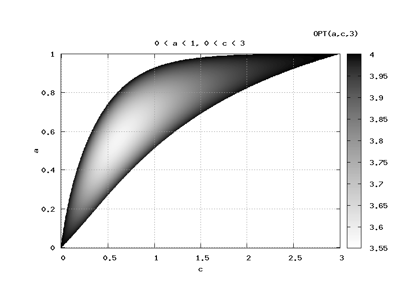
Figure 2: OPT$(a,c,s)$ over the rectangle $0\leq a\leq 1,0\leq c\leq 3$ for $s=3$ and $s=14$.

We prove four lemmas. Observe that $A(c,s)$ in Lemma 33 is a flat linear function in $c\geq 0$ from $A(0,s)=1-\frac{7}{10Q}$ to $A(3,s)=1.$

Lemma 33

$$\mbox{ Let }s\geq 7\mbox{ and let }\,A(c)\,=\,A(c,s)\,\,=\,\,\frac{7}{Q\cdot 10\cdot 3}\cdot c\,\,+1\,\,-\frac{7}{10\cdot Q}.$$

$$\mbox{Then }\,\mbox{OPT}(A(c),\,c,\,s\,)\,\mbox{ is strictly increasing in }\,\,1\leq c<3.$$

$A(c,s)$ in the subsequent Lemma is a steep linear function starting at $A(0,s)=0.$

Lemma 34

$$\mbox{ Let }s\geq 6\mbox{ and let }\,A(c)\,\,=\,\,A(c,s)\,\,=\,\,\frac{Q}{2}\cdot c\,\,.$$

$$\mbox{ Then }\,\mbox{OPT}(A(c),\,c,\,s)\,\mbox{ is strictly decreasing for }0\,<c\,\leq\,\frac{1}{Q}$$

Lemma 35

(a) For each constant $0\leq a\leq 1$ OPT$(a,c,s)$ as a function in $c$ with $0\leq c\leq 3$ has a unique local minimum.
(b) For each constant $0\leq c\leq 3$ OPT$(a,c,s)$ as a function in $a$ with $0\leq a\leq 1$ has a unique local minimum.

Lemma 36

Let $s\,\geq 6\,$ then OPT$(a,\,\,c,\,\,s\,)\,<\,4-\delta$ for $(a,\,c)\,=\,$

$$=\,\left(\frac{1}{2},\,\,\frac{1}{Q}\,\right)\,,\,\left(\frac{1}{2},\,\frac{2}{Q}\,\right),\,\,\left(\frac{2}{3},\,\frac{2}{Q}\,\right),\,\left(\frac{2}{3},\,\frac{3}{Q}\,\right),\,\left(1\,\,-\,\,\frac{7}{15Q}\,,\,\frac{3}{Q}\right),\,\,\,\left(1\,-\,\frac{7}{15Q}\,\,,\,1\,\right)$$

Proof of Theorem 28 for $\lambda\leq 1-1/d.$ (cf. proof of Theorem 9 after Lemma 20.) We have $\lambda\leq 1-1/d\Longleftrightarrow\lambda/(1-\lambda)\leq d-1.$ Using Lemma 32 we need to show that for each $P\leq d-1$ we have a decomposition $P=ac$ such that OPT$(a,c,s)\leq 4$ of $4-\delta.$ Lemma 33 treats $1-7/(15Q)\leq P\leq d-1.$ Lemma 36 together with Lemma 35 treat $1-7/(15Q)\geq P\geq 1/(2Q).$ Finally Lemma 34 treats $1/(2Q)\geq P>0.$ Observe that OPT$(0,0,s)=4$ and we need to look into the proof of Lemma 32 to get the $-\delta$ required for small $P.$ ∎

2.1 Proof of Lemma 33

Lemma 33  (repeated)

$$\mbox{ Let }s\geq 7\mbox{ and let }\,A(c)\,=\,A(c,s)\,\,=\,\,\frac{7}{Q\cdot 10\cdot 3}\cdot c\,\,+1\,\,-\frac{7}{10\cdot Q}.$$

$$\mbox{Then }\,\mbox{OPT}(A(c),\,c,\,s\,)\,\mbox{ is strictly increasing in }\,\,1\leq c<3.$$

Proof

$$\mbox{ Some notation:}\,\mbox{PPLUS3}(x,y)\,=\,(1\,+\,x)^{y}\,+\,3\left(1-\frac{x}{3}\right)^{y},\,\,x\leq 3$$

$$\mbox{PMINUS}(x,y)\,=\,(1\,+\,x)^{y}\,-\,\left(1-\frac{x}{3}\right)^{y},\,\,x\leq 3$$ (41)

$$\frac{d}{dc}\ln\mbox{PPLUS3}(c,Q)\,=\,Q\cdot\frac{\mbox{PMINUS}(c,Q-1)}{\mbox{PPLUS3}(c,Q)},\,$$

$$A\,\,=\,\,A(c),\,\,A^{\prime}\,=\,\frac{d}{dc}\,A\,=\frac{7}{10\cdot 3\cdot Q}\,\,\,,\,\,\,\frac{d}{dc}\ln\mbox{OPT}(A,c,s)\,=\,$$

$$\,=\,\frac{3\frac{\exp(As)-1)}{\exp(s)-s-1}\cdot sA^{\prime}}{\mbox{OPT}_{1}(A,s)}\,-\,Q\cdot\frac{A^{\prime}c\,+\,A}{1+Ac}\,+\,Q\cdot\frac{\mbox{PMINUS}(c,Q-1)}{\mbox{PPLUS3}(c,Q)}\,>=<0$$

$$\Longleftrightarrow\,\frac{3\frac{\exp(As)-1}{\exp(s)-1}\cdot A^{\prime}}{\mbox{OPT}_{1}(A,s)}\,-\,\frac{A+A^{\prime}c}{1+Ac}\,+\,\frac{\mbox{PMINUS}(c,Q-1)}{\mbox{PPLUS3}(c,Q)}\,>=<\,0\,\,\,\,\,\;\;\,\,\,$$ (42)

$$\mbox{(Division with }Q\,=\,\frac{s(\exp(s)-1)}{\exp(s)-s-1}\mbox{.)}$$

$$\mbox{ For }c\,=\,3\mbox{ the derivative is }=0,\,\,A(3,s)=1\,\,\mbox{( OPT}(1,3,s)=4.)$$

We split the right-hand-side of (42) into two additive terms. Inequalities (43) and (44) imply that the $\frac{d}{dc}$ OPT$(A,c,s)>0.$ For $c=3$ both left-hand-sides are $=0.$

$$\frac{3\frac{\exp(As)-1)}{\exp(s)-1}\cdot A^{\prime}}{\mbox{OPT}_{1}(A,s)}\,-\,\frac{A^{\prime}c}{1+Ac}\,>\,0$$ (43)

$$-\,\frac{A}{1+Ac}\,+\,\frac{\mbox{PMINUS}(c,Q-1)}{\mbox{PPLUS3}(c,Q)}\,>\,0$$ (44)

Proof of (43) for $0\leq c<3\,$ and $s\geq 7.$

$$K\,:=\,\frac{\exp(sA)-1}{\exp(s)-1},\,\,\,L:=\frac{\exp(sA)-sA-1}{\exp(s)-s-1}$$

$$\mbox{ We need to show }\frac{3KA^{\prime}}{3L+1}\,\,>\,\frac{A^{\prime}c}{1+Ac}\,\,\Longleftrightarrow\,\,\,\frac{3K}{3L+1}\,\,>\,\frac{c}{1+Ac}$$

$$\Longleftrightarrow\,\,3\left(K+KAc-Lc\right)\,>\,c\,\,\,\,\mbox{ (For }c=3\mbox{ both sides are }\,=3.)$$ (45)

By (7) we have $L\,\leq\,K$ and (45) is implied by

$$3K\left(1+Ac-c\right)\,>\,c\,\,\quad\mbox{ (For }c=3\mbox{ both sides are }=3.\mbox{)}$$ (46)

$K\geq 0$ is increasing and convex, $1+Ac-c$ is $>0,$ and increasing for $c>3/2,$ and convex. Therefore the left-hand-side of (46) is convex for $c\geq 3/2.$ Therefore, for $c\geq 3/2,$ it follows from

$$\left(\frac{d}{dc}3K\left(1+Ac-c\right)\right)_{|c=3}\,<\,\left(\frac{d}{dc}c\right)_{|c=3}\,=\,1.$$ (47)

$$\frac{d}{dc}3K\left(1+Ac-c\right)\,\,\,\,\,\,\,=\,\frac{3\exp(sA)\cdot s\cdot\frac{7}{30Q}}{\exp(s)-1}\cdot(1+Ac-c)\,+\,$$

$$\frac{3(\exp(sA)-1)}{\exp(s)-1}\cdot\left(\frac{7}{30Q}c+\frac{7}{30Q}c+1-\frac{7}{10Q}-1\right).$$

$$\mbox{ Therefore }\,\frac{d}{dc}3K\left(1+Ac-c\right)_{|c=3}\,=\,$$

$$\frac{7\exp(s)(\exp(s)-s-1)}{10(\exp(s)-1)^{2}}\,\,+\,\,\frac{21(\exp(s)-s-1)}{10s(\exp(s)-1)}\,\,\,\,$$ (48)

For $s=7$ we get that (48) is $<0.995.$ Moreover it is decreasing in $s$ (proof omitted) and (47) holds for all $s\geq 7$ and $c\geq 3/2.$ For $c\leq 3/2$ we argue as in the proof of Lemma 20(a) cf. the argument following (20).

Proof of (44) for $1\,\leq c\,<\,3\,$ and $s\geq 5$ .

$$\mbox{ We need to show }\frac{A}{1+Ac}\,\,<\,\frac{\mbox{PMINUS}(c,Q-1)}{\mbox{PPLUS3}(c,Q)}\,$$

$$\Longleftrightarrow A\,\cdot\,\mbox{PPLUS3}(c,Q)\,<\,(1+Ac)\mbox{PMINUS}(c,Q-1)$$

$$\Longleftrightarrow A\cdot\left(\mbox{PPLUS3}(c,Q)\,-\,c\cdot\mbox{PMINUS}(c,Q-1)\right)\,=\,A\cdot\mbox{PPLUS3}(c,Q-1)\,$$

$$<\,\mbox{PMINUS}(c,Q-1)$$

$$\Longleftrightarrow A\,<\,\frac{\mbox{PMINUS}(c,Q-1)}{\mbox{PPLUS3}(c,Q-1)}\,=\,\frac{(1+c)^{Q-1}-(1-\frac{c}{3})^{Q-1}}{(1+c)^{Q-1}+3(1-\frac{c}{3})^{Q-1}}\;\;\;\;$$ (49)

$$\mbox{(For }c=3\mbox{ both sides of (\ref{flagekl31}) are }=1.)$$

For $c=1$ inequality ( 49) becomes

$$1-\frac{7}{15Q}\,<\,\frac{2^{Q-1}-\left(\frac{2}{3}\right)^{Q-1}}{2^{Q-1}+3\left(\frac{2}{3}\right)^{Q-1}}\,=\,1-\frac{4\left(\frac{1}{3}\right)^{Q-1}}{1+3\left(\frac{1}{3}\right)^{Q-1}}$$

$$\mbox{As }\,4\left(\frac{1}{3}\right)^{Q-1}\,<\,\frac{7}{15Q}\mbox{ for }\,\,Q\geq 5,\,\,\mbox{ (\ref{flagekl31}) holds for }c=1\mbox{ and }s\geq 5\,\mbox{ as }Q\geq s.$$

To show that (49) holds for all $3\,>\,c\geq\,\,1$ we show that the right-hand-side is concave for $c>1.$

$$\mbox{ Numerator of }\frac{d}{dc}\frac{\mbox{PMINUS}(c,Q-1)}{\mbox{PPLUS3}(c,Q-1)}\,=\,$$

$$(Q-1)\cdot\left((1+c)^{Q-2}\,+\,\frac{1}{3}\left(1-\frac{c}{3}\right)^{Q-2}\right)\cdot\left((1+c)^{Q-1}\,+\,3\left(1-\frac{c}{3}\right)^{Q-1}\right)\,-\,$$

$$\,-\,(Q-1)\cdot\left((1+c)^{Q-1}\,-\,\left(1-\frac{c}{3}\right)^{Q-1}\right)\cdot\left((1+c)^{Q-2}\,-\,\left(1-\frac{c}{3}\right)^{Q-2}\right)\ \,$$

$$\,=\,(Q-1)\cdot(1+c)^{Q-2}\cdot\left(1-\frac{c}{3}\right)^{Q-2}\cdot\left(\left(\frac{1}{3}+1\right)(1+c)\,+\,\left(1-\frac{c}{3}\right)\cdot(1+3)\right)\,\,$$

$$\,=\,(Q-1)\cdot(1+c)^{Q-2}\cdot\left(1-\frac{c}{3}\right)^{Q-2}\cdot\left(\frac{1}{3}+3+2\right)\;\;\;\;\;$$ (50)

$$\mbox{ We have that }(1+c)\cdot\left(1-\frac{c}{3}\right)\mbox{ is decreasing for }c>1,\mbox{ and PPLUS3}(c,Q-1)\mbox{ is increasing }.$$

Therefore the right-hand-side of (49) is concave.

2.2 Proof of Lemma 34

Lemma 34  (repeated)

$$\mbox{ Let }s\geq 6\mbox{ and let }\,A(c)\,\,=\,\,A(c,s)\,\,=\,\,\frac{Q}{2}\cdot c\,\,.$$

$$\mbox{ Then }\,\mbox{OPT}(A(c),\,c,\,s)\,\mbox{ is strictly decreasing for }0\,<c\,\leq\,\frac{1}{Q}$$

Proof

Analogously to (43) and (44) this follows from (51) and (52.) (Notation cf. ( 41.)

$$\mbox{ with }A=A(c),\,\,A^{\prime}\,=\,\,Q/2\,\,\frac{3\frac{\exp(As)-1)}{\exp(s)-1}}{\mbox{OPT}_{1}(A,\,s)}A^{\prime}\,-\,\frac{A^{\prime}c}{1+Ac}\,\,<\,\,0,\,$$ (51)

$$-\,\frac{A}{1+Ac}\,+\,\frac{\mbox{PMINUS}(c,Q-1)}{\mbox{PPLUS3}(c,Q)}\,<\,0.$$ (52)

Proof of (51) for $s\geq 5.55\,\,$ and $0\,<\,c\,\leq\,1/Q$

$$K\,:=\,\frac{\exp(sA)-1}{\exp(s)-1},\,\,\,L:=\frac{\exp(sA)-sA-1}{\exp(s)-s-1}$$

$$\mbox{ We need to show }\frac{3KA^{\prime}}{3L+1}\,\,<\,\frac{A^{\prime}c}{1+Ac}\,\,\Longleftrightarrow\,\,\frac{3K}{3L+1}\,\,<\,\frac{c}{1+Ac}$$

$$\Longleftrightarrow\,\,3\left(K+KAc-Lc\right)\,<\,c\mbox{ For }c=0\mbox{ both sides are }\,=0.$$ (53)

As $AK\leq L$ by (7) we get that (53) is implied by $3\cdot K<c.$ For $c=0$ both sides of $3\cdot K<c$ are $0.$ The left-hand-side is convex. It is sufficient to show $3\cdot K<c.$ for $c=1/Q.$ Plugging in the definition of $1/Q$ for $c$ and $A(1/Q\,,s)\,=\,1/2$ into $K$ we need to show

$$\frac{3\exp(s/2)-1}{\exp(s)-1}<\frac{\exp(s)-s-1}{s(\exp(s)-1)}\,\Longleftrightarrow\,3s\exp(s/2)\,<\,\exp(s)-1$$

For $s\geq 6$ the preceding inequality holds by simple consideration.

Proof of (52) for $s\geq 2\,\,$ and $c\leq 1/Q$ Analogously to the proof of (49) we need to show

$$A\,=\,\frac{Q}{2}c\,>\,\frac{\mbox{PMINUS}(c,Q-1)}{\mbox{PPLUS3}(c,Q-1)}\,=\,\frac{(1+c)^{Q-1}-(1-\frac{c}{3})^{Q-1}}{(1+c)^{Q-1}+3(1-\frac{c}{3})^{Q-1}}\;\;\;\;$$ (54)

$$\mbox{ For }c=0\mbox{ both sides of the preceding inequality are }=0$$

We show, that $A^{\prime}\,>$ the derivative wrt. $c$ of the right-hand-side of (54). Using (50) we need to show

$$\frac{Q}{2}\cdot\left((1+c)^{Q-1}+3\left(1-\frac{c}{3}\right)^{Q-1}\right)^{2}\,\,>\,\,(Q-1)\cdot(1+c)^{Q-2}\cdot\left(1-\frac{c}{3}\right)^{Q-2}\cdot\frac{16}{3}.$$

$$\mbox{Note }\,Q\cdot(1+c)^{Q-1}\cdot\left(1-\frac{c}{3}\right)^{Q-1}\cdot\frac{16}{3}\geq(Q-1)\cdot(1+c)^{Q-2}\cdot\left(1-\frac{c}{3}\right)^{Q-2}\cdot\frac{16}{3}$$

$$\mbox{ as }\,\,\,(1+c)\cdot\left(1-\frac{c}{3}\right)\geq 1\mbox{ for }0\leq c\leq 1/Q<2.$$

Enlarging the right-hand-side it is sufficient to show

$$3\left((1+c)^{Q-1}+3\left(1-\frac{c}{3}\right)^{Q-1}\right)^{2}\,>\,(1+c)^{Q-1}\cdot\left(1-\frac{c}{3}\right)^{Q-1}\cdot 32.$$

$$\Longleftrightarrow 3\left(1+3\left(\frac{1-\frac{c}{3}}{1+c}\right)^{Q-1}\right)^{2}\,>\,32\cdot\left(\frac{1-\frac{c}{3}}{1+c}\right)^{Q-1}$$

Setting $x=\left(\frac{1-\frac{c}{3}}{1+c}\right)^{Q-1}$ it is easy to see that the preceding inequality holds for $x\geq 0,$ and therefore clearly for $c\leq 1/Q<3.$

2.3 Proof of Lemma 36 and Lemma 35

Lemma 35 follows by elementary consideration, see the analogous situation in the proof of Lemma 18(a) and Lemma 19 (a).

Lemma 36  (repeated) Let $s\,\geq 6\,$ then OPT$(a,\,\,c,\,\,s\,)\,<\,4-\delta$ for $(a,\,c)\,=\,$

$$=\,\left(\frac{1}{2},\,\,\frac{1}{Q}\,\right)\,,\,\left(\frac{1}{2},\,\frac{2}{Q}\,\right),\,\,\left(\frac{2}{3},\,\frac{2}{Q}\,\right),\,\left(\frac{2}{3},\,\frac{3}{Q}\,\right),\,\left(1\,\,-\,\,\frac{7}{15Q}\,,\,\frac{3}{Q}\right),\,\,\,\left(1\,-\,\frac{7}{15Q}\,\,,\,1\,\right)$$

Proof

The claim for $a=\frac{1}{2},\,\,c\,=\,\frac{1}{Q}$ is included in Lemma 34.

$$\mbox{FIRSUM}(a,c,s)\,=\,(1+c)^{Q}\mbox{OPT}_{2}(a,c,s)\,\,=\,\,\left(\frac{1+c}{1+ac}\right)^{Q}$$

$$\mbox{SECSUM}(a,c,s)\,=\,3\left(1-\frac{c}{3}\right)^{Q}\mbox{OPT}_{2}(a,c,s)\,=\,3\left(\frac{1-\frac{c}{3}}{1+ac}\right)^{Q}\mbox{ then }$$

$$\mbox{OPT}(a,c,s)\,=\,\mbox{OPT}_{1}(a,s)\cdot\left[\mbox{FIRSUM}(a,c,s)\,+\,\,\mbox{SECSUM}(a,c,s)\right].$$

$$\mbox{For }x,y\geq 0\,\mbox{ we have }\mbox{FIRSUM}\left(x,\frac{y}{Q},s\right)\,=\,\,\left(\frac{1+\frac{y}{Q}}{1+x\cdot\frac{y}{Q}}\right)^{Q}\,=\,\,\,$$

$$=\,\,\left(1\,+\,\frac{\frac{y}{Q}(1-x)}{1+x\frac{y}{Q}}\right)^{Q}\,\,\leq\,\exp\left(\frac{y(1-x)}{1+x\frac{y}{Q}}\right)\leq\,\exp(y(1-x))$$ (55)

$$\mbox{ We have that OPT}_{1}(a,s)\mbox{is decreasing in }s\mbox{ for constant }a<1.$$ (56)

$$\mbox{ Let }\,a=\frac{1}{2},\,\,c\,=\,\frac{2}{Q}.$$

$$\mbox{ We have by (\ref{bFIR}) }\mbox{FIRSUM}(a,c,s)\,<\,\exp(1)$$

$$\mbox{SECSUM}(a,c,s)\mbox{ is decreasing in }s\geq 0.$$

(As can be shown by elementary means.)

$$\mbox{OPT}_{1}(a,s)\left(\mbox{SECSUM}(a,c,s)+\exp(1)\right)\,<\,3.913\,\mbox{ for }s=5$$

$$\mbox{ and decreasing in }s\mbox{ with (\ref{OPT1dec})}$$

$$\mbox{ Let }\,a=\frac{2}{3},\,\,c\,=\,\frac{2}{Q}.$$

$$\mbox{ We have }\,\mbox{FIRSUM}(a,c,s)\,<\,\exp(2/3)$$

$$\mbox{SECSUM}(a,c,s)\mbox{ is decreasing in }s\geq 0.\,\,$$

$$\mbox{OPT}_{1}(a,s)\left(\mbox{SECSUM}(a,c,s)+\exp(2/3)\right)\,<\,3.962\,\mbox{ for }s=4$$

$$\mbox{ and decreasing in }s\mbox{ with (\ref{OPT1dec})}$$

$$\mbox{ Let }\,a=\frac{2}{3},\,\,c\,=\,\frac{3}{Q}.\mbox{ We have }\mbox{FIRSUM}(a,c,s)\,<\,\exp(1)$$

$$\mbox{SECSUM}(a,c,s)\mbox{ is decreasing in }s\geq 2.\,\,$$

$$\mbox{OPT}_{1}(a,s)\left(\mbox{SECSUM}(a,c,s)+\exp(1)\right)\,<\,3.985\,\mbox{ for }s=6$$

$$\mbox{ and decreasing in }s\mbox{ with (\ref{OPT1dec})}$$

$$\mbox{ Let }a=1-7/(15Q),\,c=3/Q.$$

$$\mbox{OPT}_{1}(a,s)\mbox{ is increasing in }s\mbox{ to }3\exp(-7/15)+1.$$

$$\mbox{FIRSUM }(a,c,s),\,\mbox{SECSUM}(a,c,s)\mbox{are both decreasing in }s.$$

$$(3\exp(-7/15)+1)\left(\mbox{SECSUM}(a,c,s)+\mbox{FIRSUM}(a,c,s)\right)\,<\,3.9\mbox{ for }s=4$$

The case $a=1\,-\,\frac{7}{15Q}$ and $c=1\,$ is included in Lemma 33.

3 Proof of Theorem 28 for $d=4,\,\lambda\geq 1-1/d,s\geq 5.$

We fix $a=1.$ Observe that $B(1/c)$ in the subsequent lemma goes from $1$ to $1-1/(2Q)$ for $c\geq 3.$

Lemma 37

Let $B(x)\,=\,B(x,s)\,=\,1+3/(2Q)x-1/(2Q).$ Then OPT$(1,B(1/c),c,s)$ is strictly decreasing in $c\geq 3.$

Proof of Theorem 28 for $\lambda\geq 1-1/d.$ We have $\lambda/(1-\lambda)\geq d-1.$ For each $P\geq d-1$ we have $c$ such that $P\,=\,\frac{c}{B(1/c)}.$ As OPT$(1,1,3,s)=4$ the Theorem follows. ∎

Proof of Lemma 37. We rewrite OPT$(1,B(1/c),c,s)$ first. We multiply OPT₂ with $c^{Q}$ and OPT₃ with $1/c^{Q}$ and get (using $c\geq 3$ to get rid of the absolute value) OPT$(1,B(1/c,s),c,s)\,=\,$

$$=\,\left(3+\frac{q(B(1/c,s)s)}{q(s)}\right)\left(\frac{1}{\frac{B(1/c,s)}{c}+1}\right)^{Q}\left(\left(\frac{1}{c}+1\right)^{Q}+3\left(\frac{1}{3}-\frac{1}{c}\right)^{Q}\right).$$

$$\mbox{ We substitute }c\mbox{ for }1/c\mbox{ in the preceding equation. The claim follows from }$$

$$\left(3+\frac{q(B(c))s)}{q(s)}\right)\left(\frac{1}{B(c)c+1}\right)^{Q}\left(\left(c+1\right)^{Q}+3\left(\frac{1}{3}-c\right)^{Q}\right)$$

$$\mbox{increases in }0\,<\,c\,<\,1/3.$$ (57)

We use the following notation in the sequel:

$$\mathrm{OPT}_{1}(b,s)=3+\frac{q(sb)}{q(s)}\,,\,\mathrm{OPT}_{2}(b,c,s)\,=\,\left(\frac{1}{bc+1}\right)^{Q},$$

$$\mathrm{OPT}_{3}(c,s)=(c+1)^{Q}+\,3\left(\frac{1}{3}-c\right)^{Q},\,c\leq\frac{1}{3}$$

$$\mathrm{OPT}(b,c,s)=\mathrm{OPT}_{1}(b,s)\mathrm{OPT}_{2}(b,c,s)\mathrm{OPT}_{3}(c,s).$$

$$\mbox{ For }b=1,c=\frac{1}{3}\mbox{ we have }\mathrm{OPT}(b,c,s)=4.\mbox{ We abbreviate }$$

$$\mbox{PM}(x,y)=(x+1)^{y}-3\left(\frac{1}{3}-x\right)^{y},\,x\leq\frac{1}{3}$$

$$\mbox{PP}(x,y)=(x+1)^{y}+3\left(\frac{1}{3}-x\right)^{y},\,x\leq\frac{1}{3}$$

$$B\,=B(c,s),\quad B^{\prime}=\frac{\partial}{\partial c}B=\frac{3}{2Q},\quad q^{\prime}(x)=\exp(x)-1$$

$$q(x)=\exp(x)-x-1,\,\,\,\,\,\frac{\partial}{\partial c}\ln(\mathrm{OPT}(B,c,s)>=<0$$

$$\Longleftrightarrow\frac{\frac{B^{\prime}sq^{\prime}(sB)}{q(s)}}{3+\frac{q(sB)}{q(s)}}\,-Q\frac{B^{\prime}c+B}{1+Bc}+Q\frac{\mbox{PM}(c,Q-1)}{\mbox{PP}(c,Q)}>0$$

$$\Longleftrightarrow\frac{\frac{B^{\prime}q^{\prime}(sB)}{q^{\prime}(s)}}{3+\frac{q(sB)}{q(s)}}-\frac{B^{\prime}c+B}{1+Bc}+\frac{\mbox{PM}(c,Q-1)}{\mbox{PP}(c,Q)}>=<0.\mbox{( Division by }Q.)$$ (58)

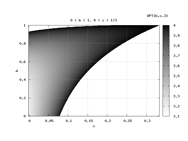
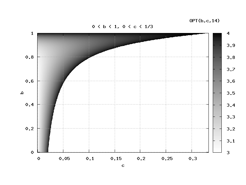
Figure 3: OPT$(b,c,s)$ over the rectangle $0\leq b\leq 1,0\leq c\leq 1/3$ for $s=3$ and $s=14$.

For $c=\frac{1}{3}$ we have $\mathrm{OPT}(B,1/3,s)=4$, and the derivative is $0$. We split (58) into two additive terms. The following two inequalities directly imply (57.)

$$\frac{\frac{B^{\prime}q^{\prime}(sB)}{q^{\prime}(s)}}{3+\frac{q(sB)}{q(s)}}-\frac{B^{\prime}c}{1+Bc} > 0$$ (59)

$$\frac{\mbox{PM}(c,Q-1)}{\mbox{PP}(c,Q)}-\frac{B}{1+Bc} > 0$$ (60)

Proof of (59) for $\,s>2\,.$ Let $K=\frac{q^{\prime}(sB)}{q^{\prime}(s)}$ and $L=\frac{q(sB)}{q(s)}.$ By (7) we have $L\leq K,$ and as $B^{\prime}>0$ it is sufficient to show

$$\frac{K}{3+K}>\frac{c}{1+Bc}\Leftrightarrow K(1+Bc-c)>3c.$$

For $c=\frac{1}{3}$ both sides of the preceding inequality are $=1$. It is easy to observe that $K(1+Bc-c)$ is convex in $c$ for $c>1/(3\cdot 2).$ (Cf. proof of Lemma 20) and $3c$ is a linear function. If at $c=\frac{1}{3}$ the derivative of $3c$ is greater than the derivate of $K(1+Bc-c)$ the second intersection of both sides (if any) lies at some point $c>\frac{1}{3}$ and the claim holds for $1/(3\cdot 2<c<\frac{1}{3}$. For $c<1/(3\cdot 2)$ we argue as in the proofs of the Lemmas mentioned above. Therefore it is sufficient to show that at $c=\frac{1}{3}$

$$\frac{\partial}{\partial c}K(1+Bc-c)<\frac{\partial}{\partial c}3c.$$

We have

$$K^{\prime}=\frac{B^{\prime}s\exp(sB)}{\exp(s)-1}.$$

and at $c=1/3$

$$K^{\prime}(\underbrace{1+Bc-c}_{=1})+\underbrace{K}_{=1}(\underbrace{B^{\prime}c+B-1}_{=1/2Q}) < 3$$

$$\Leftrightarrow\frac{3(\exp(s)-s-1)\exp(s)}{2(\exp(s)-1)^{2}}+\frac{\exp(s)-s-1}{2s(\exp(s-1)} < 3$$ (61)

We omit the proof that inequality (61) holds for $s\geq 2.$

Proof of (60) for $s\geq 5$. As in (49) inequality (60) is equivalent to

$$B<\frac{\mbox{PM}(c,Q-1)}{\mbox{PP}(c,Q-1}$$ (62)

The left hand side is a linear function in c and the right hand side a strictly increasing, concave function in $c.$ For $c=\frac{1}{3}$ both sides of (62) are $1$. So we must show that (62) holds for $c=0$. Setting $c=0$ leads to

$$1-\frac{1}{2Q}<\frac{1-3\left(\frac{1}{3}\right)^{Q-1}}{1+3\left(\frac{1}{3}\right)^{Q-1}}=\frac{1-\left(\frac{1}{3}\right)^{Q-2}}{1+\left(\frac{1}{3}\right)^{Q-2}}.$$

For $Q=5$ we get $\frac{9}{10}<\frac{13}{14}$. We omit the argument that the last inequality holds for all $Q\geq 5$ and therefore as $Q>s$ for all $s\geq 5.$

References

[1] J. Diaz et al. On the satisfiability threshold of formulas with three literals per clause. Theoretical Computer Science 410 (2009) 2920 - 2934.
[2] M Molloy. Cores in random hypergraphs and boolean formulas. Random Stuctures and Algorithms 27, 2005, 124 - 135.
[3] J. Hastad. Some optimal inapproximability results. J. ACM 48, 2001, 798 – 859.
[4] R. Durrett. Probability Theory: Theory and Examples. Wadsworth and Brooks 1991.
[5] M Dietzfelbinger et al. Tight thresholds for Cuckoo Hashing via XORSAT. CoRR, 2009, abs/0912.0287. See also
Proceedings ICALP 2010, LNCS 6198, 213 - 225.
[6] H. Connamacher, M. Molloy. The exact satisfiability
threshold for a potentially in tractable random constraint satisfaction problem. Proceedings 45th FoCS 2004, 590 - 599.
[7] Michael Molloy. Models for Random Constraint Satisfaction Problems. SIAM J. Comput. 32(4), 2003, 935-949.
[8] O. Dubois, J. Mandler. The XORSAT satisfiability threshold. Proceedings 43rd FoCS 2003, 769.
[9] N. Creignou, H. Daudé. The SAT-UNSAT transition for random constraint satisfaction problems. Discrete Mathematics 309 (8),
2085 - 2099.
[10] V. F. Kolchin. Random graphs and systems of linear equations in finite fields.
Random Structures and Algorithms 5, 1995, 425 - 436.
[11] A. Braunstein, M. Mezard, R. Zecchina. Survey propagation: an algorithm for satisfiability. arXiv:cs/0212002.
[12] Amin Coja-Oghlan, Angelica Y. Pachon-Pinzon. The Decimation Process in Random k-SAT. In Proceedings ICALP (1) 2011, 305-316.
[13] Ehud Friedgut. Hunting for sharp thresholds. Random Struct. Algorithms 26(1-2), 2005, 37-51.
[14] Andreas Goerdt. On Random Betweenness Constraints. Combinatorics, Probability and Computing 19(5-6), 2010, 775-790
[15] D. Achlioptas, C. Moore. Random k-SAT: Two Moments Suffice to Cross a Sharp Threshold. SIAM J. Comput. 36(3), 2006, 740-762
[16] V. Puyhaubert. Generating functions and the satisfiability threshold. Discrete Mathematics and Theoretical Computer Science 6, 2004, 425, - 436.
[17] H. Connamacher. Exact thresholds for DPLL on random XOR-SAT and NP-complete extensions of XOR-SAT. Theoretical Computer Science 2011.
[18] A. Meisels, S. E. Shimony, G. Solotorevsky. Bayes Networks for estimating the number of solutions to a CSP. Proceedings AAAI 1997, 179 - 184.
[19] M. Luby, M. Mitzenmacher, A. Shokrollahi, D. A. Spielman. Efficient erasure coeds. IEEE Trans. Inform. Theory 47(2), 2001, 569 - 584.
[20] T. J. Richardson, R. Urbanke. Modern Coding Theory. Cambridge University Press, 2008.
[21] Dimitris Achlioptas, Morteza Ibrahimi, Yashodhan Kanoria, Matt Kraning, Mike Molloy and Andrea Montanari. The Set of Solutions of Random XORSAT Formulae. In Proceedings SoDA 2012.
[22] N. G. de Bruijn. Asymptotic Methods in Analysis. North Holland 1958,
[23] N. Bhattacharya, R. Ranga Rao. Normal Approximation and Asymptotic Expansions. Robert E. Krieger Publishing Company, 1986.
[24] M. Mitzenmacher, Eli Upfal. Probability and Computing: Randomized Algorithms and Probabilistic Analysis.
Cambridge University Press 2005.