Incremental Slow Feature Analysis: Adaptive and Episodic Learning from High-Dimensional Input Streams

Varun R. Kompella, Matthew Luciw and J$\ddot{\mbox{u}}$ergen Schmidhuber

Technical Report No. IDSIA-07-11

November 2011

IDSIA / USI-SUPSI
Istituto Dalle Molle di studi sull’intelligenza artificiale
Galleria 2, 6928 Manno, Switzerland

  IDSIA was founded by the Fondazione Dalle Molle per la Qualità della Vita and is affiliated with both the Università della Svizzera italiana (USI) and the Scuola unversitaria professionale della Svizzera italiana (SUPSI).

Incremental Slow Feature Analysis: Adaptive and Episodic Learning from High-Dimensional Input Streams

Slow Feature Analysis (SFA) extracts features representing the underlying causes of changes within a temporally coherent high-dimensional raw sensory input signal. Our novel incremental version of SFA (IncSFA) combines incremental Principal Components Analysis and Minor Components Analysis. Unlike standard batch-based SFA, IncSFA adapts along with non-stationary environments, is amenable to episodic training, is not corrupted by outliers, and is covariance-free. These properties make IncSFA a generally useful unsupervised preprocessor for autonomous learning agents and robots. In IncSFA, the CCIPCA and MCA updates take the form of Hebbian and anti-Hebbian updating, extending the biological plausibility of SFA. In both single node and deep network versions, IncSFA learns to encode its input streams (such as high-dimensional video) by informative slow features representing meaningful abstract environmental properties. It can handle cases where batch SFA fails.

1 Introduction

Slow feature analysis (Wiskott and Sejnowski, 2002; Wiskott et al., 2011)(SFA) is an unsupervised learning technique that extracts features from an input stream with the objective of maintaining an informative but slowly-changing feature response over time. The idea of using temporal stability as an objective in learning systems has motivated some other unsupervised learning techniques (Hinton, 1989; Földiák, 1991; Mitchison, 1991; Schmidhuber, 1992a; Bergstra and Bengio, 2009). SFA is distinguished by its formulation of the feature extraction problem as an eigensystem problem, which guarantees that its solution methods reliably converge to the best solution, given its constraints (no local minima problem). SFA has shown success in problems such as extraction of driving forces of a dynamical system (Wiskott, 2003), nonlinear blind source separation (Sprekeler et al., 2010), as a preprocessor for reinforcement learning (Legenstein et al., 2010; Kompella et al., 2011b), and learning of place-cells, head-direction cells, grid-cells, and spatial view cells from high-dimensional visual input (Franzius et al., 2007) — such representations also exist in biological agents (O’Keefe and Dostrovsky, 1971; Taube et al., 1990; Rolls, 1999; Hafting et al., 2005).

There are limitations to existing SFA implementations due to their batch processing nature, which becomes especially apparent when attempting to apply it in somewhat uncontrolled environments. To overcome these issues, we introduce the new Incremental Slow Feature Analysis (IncSFA) (Kompella et al., 2011a, b). A few earlier techniques with temporal continuity objective were incremental as well (Hinton, 1989; Bergstra and Bengio, 2009), but IncSFA follows the SFA formulation and can track solutions of batch SFA (BSFA), over which it has the following advantages:

• Adaptation to changing input statistics. BSFA requires all data to be collected in advance. New data cannot be used to modify already learned slow features. Once the input statistics change, IncSFA can automatically adapt its features without outside intervention, while BSFA has to discard previous features to process the new data.

  In open-ended learning settings, an autonomous agent’s lifelong input stream follows such a nonstationary distribution. The agent’s behavior will typically change over time, thus generating new input sequences. Features useful for early behaviors may not be useful for later behavior.

• Learn features across episodes. Episodic learning is impossible for BSFA, since it cannot handle temporal discontinuities at episode boundaries. IncSFA, however, may use the final slow features from the previous episode to initialize its features of the next episode.

• Reduced sensitivity to outliers. Real-world environments typically exhibit infrequent, uncontrolled, insignificant external events that should be ignored. BSFA is very sensitive to such events, encoding everything that changes slowly within the current batch. IncSFA’s plasticity, however, makes it lose sensitivity to such events over time.

• Covariance-free. BSFA techniques rely upon batch Principal Component Analysis (Jolliffe, 1986) (PCA), which requires the data’s covariance matrix. Estimating, storing and/or updating covariance matrices can be expensive for high-dimensional data and impractical for open-ended learning. IncSFA uses covariance-free techniques. For high-dimensional images, the number of parameters to estimate in the covariance matrix is huge: $n(n+1)/2$ for dimension $n$, while a covariance-free technique only requires $n\times m$ where $m$ is the desired number of principal components (PCs). For example, $100\times 100$ dimensional images lead to $50,005,000$ free parameters in the covariance matrix, which is reduced to only $100\times 100\times m$ eigenvector parameters with covariance-free updating.

  Furthermore, since often only a relatively small number of principal components are needed to explain most of the variance in the data, the other components do not even have to be estimated. With IncSFA, dimensionality reduction can be done during PC estimation; no time needs to be wasted on computing the many insignificant lower-order PCs.

  Another technical problem with the covariance matrix: in sequences where only a small part of the input changes, computing the principal components of the difference signal’s covariance matrix will result in singularity errors, since the matrix won’t have full rank.

• Biological Plausibility. IncSFA adds further biological plausibility to SFA. SFA itself is linkable to biological systems due to the results in deriving place cell, grid cells, etc., but it is difficult to see how BSFA could be realized in the brain. IncSFA’s updates, however, can be described in incremental Hebbian and anti-Hebbian terms.

The remainder of this paper is organized as follows. Section 2 reviews SFA and its batch solution. Section 3 describes the new incremental SFA. Section 4 details the algorithm and discusses deeper related issues, including convergence conditions and parameter setting. Section 5 contains experiments and results, and shows how to utilize IncSFA as part of a hierarchical image processing architecture. Section 6 concludes the paper.

2 Background

2.1 SFA: Intuition

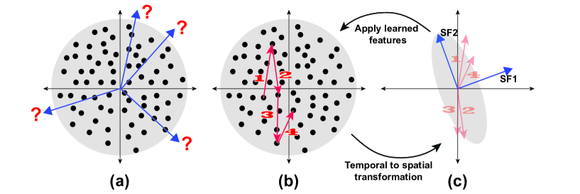
Figure 1: Intuition of SFA. (A): Consider a zero-mean input signal that spatially resembles white noise. Assume the input distributions are Gaussian, shown by the gray area, while the black dots show individual data points. Spatial feature extractors such as PCA will not prefer any direction over any other. (B): Eschewing unhelpful spatial processing, we examine this input as a time-series; to illustrate here we show a short sequence of input. Each difference vector becomes a spatial component in the space shown in (C). In this space, the first principal component gives the (linear) direction of quickest change. The second — the minor component — gives the direction of slowest change. We see that recoding the data in terms of subsequent differences and performing an eigendecomposition provides an ordered set of separate features, which are applied to the original input signal.

We first review SFA briefly in an intuitive sense. SFA is a form of unsupervised learning (UL). It searches for a set of mappings $g_{i}$from data ${\bf x}\in\mathcal{R}^{I}$ to output components $y_{i}=g_{i}({\bf x})$ that are separate from each other in some sense and express information that is in some sense relevant. In SFA separateness is realized as decorrelation (like in PCA), while relevance is defined in terms of slowness of change over time. Ordering our functions $g_{1},g_{2},...,g_{I}$ by slowness, we can discard all but the $J<I$ slowest, to enable dimensionality reduction, getting rid of irrelevant information such as quickly changing noise assumed to be useless. The compact relevant data encodings reduce the search space for downstream goal-directed learning procedures (Schmidhuber, 1999; Barlow, 2001). As an example, consider a high-dimensional dynamical system: a mobile robot sensing with an onboard camera, where each pixel is considered a separate observation component. SFA will use the video sequences to guide its search over functions that encode each image into a small set of state variables, and the robot can use these new state variables to quickly develop useful controllers. Fig. 1 provides a visual example of how SFA operates.

SFA-based UL learns instantaneous features from sequential data (Hinton, 1989; Wiskott and Sejnowski, 2002; Doersch et al., ). Relevance cannot be uncovered without taking time into account, but once it is known, each input frame can be processed on its own. SFA differs from both 1. many well-known unsupervised feature extractors (Abut, 1990; Jolliffe, 1986; Comon, 1994; Lee and Seung, 1999; Kohonen, 2001; Hinton, 2002), which ignore dynamics, and 2. Other UL systems that both learn and apply features to sequences (Schmidhuber, 1992a, c, b; Lindstädt, 1993; Klapper-Rybicka et al., 2001; Jenkins and Matarić, 2004; Lee et al., 2010; Gisslen et al., 2011), thus assuming that the state of the system itself can depend on past information.

2.2 SFA: Formulation

SFA’s optimization problem (Wiskott and Sejnowski, 2002; Franzius et al., 2007) is formally written as follows:

Given an I-dimensional sequential input signal ${\bf x}(t)=[x_{1}(t),...,x_{I}(t)]^{T}$, find a set of $J$ instantaneous real-valued functions ${\bf g}(x)=[g_{1}({\bf x}),...,g_{J}({\bf x})]^{T}$, which together generate a $J$-dimensional output signal ${\bf y}(t)=[y_{1}(t),...,y_{J}(t)]^{T}$ with $y_{j}(t):=g_{j}({\bf x}(t))$, such that for each $j\in\{1,...,J\}$

$$\Delta_{j}:=\Delta(y_{j}):=\langle\dot{y}_{j}^{2}\rangle\quad\textrm{is minimal}$$ (1)

under the constraints

$$\langle y_{j}\rangle = 0\quad\textrm{(zero mean),}$$ (2)

$$\langle y_{j}^{2}\rangle = 1\quad\textrm{(unit variance),}$$ (3)

$$\forall i<j:\langle y_{i}y_{j}\rangle = 0\quad\textrm{(decorrelation and order),}$$ (4)

with $\langle\cdot\rangle$ and $\dot{y}$ indicating temporal averaging and the derivative of $y$, respectively.

The problem is to find instantaneous functions $g_{j}$ that generate different output signals varying as slowly as possible. The constraints (2) and (3) together avoid a trivial constant output solution. The decorrelation constraint (4) ensures that different functions $g_{j}$ do not code for the same features.

2.3 Batch SFA

Solving this learning problem involves non-trivial variational calculus optimization. But it is simplified through an eigenvector approach. If the $g_{j}$ are linear combinations of a finite set of nonlinear functions ${\bf h}$, then

$$y_{j}(t)=g_{j}({\bf x}(t))={\bf w}^{T}_{j}~{}{\bf h}({\bf x}(t))={\bf w}^{T}_{j}~{}{\bf z}(t),$$ (5)

and the SFA problem now becomes to find weight vectors ${\bf w}_{j}$ to minimize the rate of change of the output variables,

$$\Delta(y_{j})=\langle\dot{y}_{j}^{2}\rangle={\bf w}_{j}^{T}~{}\langle\dot{{\bf z}}\dot{{\bf z}}^{T}\rangle~{}{\bf w}_{j},$$ (6)

subject to the constraints (2-4). The slow feature learning problem has become linear on the derivative signal $\dot{{\bf z}}$.

If the functions of ${\bf h}$ are chosen such that ${\bf z}$ has unit covariance matrix and zero mean, the three constraints will be fulfilled if and only if the weight vectors ${\bf w}_{j}$ are orthonormal. Eq. 6 will be minimized, and the orthonormal constraint satisfied, with the set of $J$ normed eigenvectors of $\langle\dot{{\bf z}}\dot{{\bf z}}^{T}\rangle$ with the $J$ smallest eigenvalues (for any $J\leq I$).

The BSFA technique practically implements this solution by using batch principal component analysis (PCA) (Jolliffe, 1986) twice. Referring back to Eq. 6, to select ${\bf h}$ appropriately, a well-known process called whitening (or sphering), is used to map ${\bf x}$ to a ${\bf z}$ with zero mean and identity covariance matrix, thus decorrelating signal components and scaling them so that there is unit variance along each PC direction. Whitening serves as a bandwidth normalization, so that slowness can truly be measured (slower change will not simply be due to a low variance direction). Whitening requires the PCs of the input signal (PCA #1). The orthonormal basis that minimizes the rate of output change are the minor components – principal components with smallest eigenvalues – in the derivative space. So another PCA (#2) on $\dot{{\bf z}}$ yields the slow features (eigenvectors) and their order (via eigenvalues).

3 Incremental SFA

IncSFA also employs the eigenvector tactic, but may update an existing estimate on any amount of new data, even a single data point ${\bf x}(t)$. A high-level formulation is

$$({\bf W}(t+1),\theta(t+1))=IncSFA({\bf W}(t),{\bf x}(t),\theta(t)),$$ (7)

where ${\bf W}=\left({\bf w}_{1},...,{\bf w}_{J}\right)$ is the matrix of existing slow feature vector estimates, and $\theta$ contains algorithm memory and parameters, which we will discuss later.

To replace PCA $\#1$, IncSFA needs to do online whitening of input ${\bf x}$. We use Candid Covariance-Free Incremental (CCI) PCA (Weng et al., 2003). CCIPCA incrementally updates both the eigenvectors and eigenvalues necessary for whitening, and does not keep an estimate of the covariance matrix. CCIPCA is also used to reduce dimensionality.

Except for low-dimensional derivative signals $\dot{{\bf z}}$, CCIPCA cannot replace PCA $\#2$. It will be unstable, since the slow features correspond to the least significant components. Minor Components Analysis (MCA) (Oja, 1992) incrementally extracts the principal components with the smallest eigenvalues. We use Peng’s low complexity updating rule (Peng et al., 2007). Peng proved its convergence even for constant learning rates—good for open-ended learning. MCA with sequential addition (Chen et al., 2001; Peng and Yi, 2006) will extract multiple slow features in parallel.

3.1 Neural Updating for PC and MC Extraction

CCIPCA and Peng’s MCA are the most appropriate incremental PCA and MCA algorithms for IncSFA. To justify these choices, we briefly review the literature on neural networks that perform incremental PCA and MCA.

Well-known incremental PCA algorithms are Oja and Karhunen’s Stochastic Gradient Ascent (SGA) (Oja, 1985), Sanger’s Generalized Hebbian Algorithm (GHA) (Sanger, 1989), and CCIPCA. They all build on the work of Amari (1977) and Oja (1982), who showed that a linear neural unit using Hebbian updating could compute the first principal component of a data set (Amari, 1977; Oja, 1982). However, SGA (1985) builds upon Oja’s earlier work, GHA (1989) builds upon SGA, and CCIPCA (2003) builds upon GHA.

SGA use Gram-Schmidt Orthonormalization (GSO) to incrementally find the subspace of all principal components, but there is no guarantee of finding the components themselves. Sanger used Kreyszig’s (Kreyszig, 1988) (1988) (faster/more effective) residual vector method for computing multiple components. His provably converging GHA used the residual method for simultaneous computation of all components. CCIPCA (Weng et al., 2003) modified GHA to be “candid”, meaning it maintained an implicit learning rate dependant on the data, greatly increasing the algorithm’s efficiency so that it became useful for high-dimensional inputs, such as in appearance-based computer vision. This incremental PCA updating method is the best of the above for IncSFA. It converges (Zhang and Weng, 2001) to both eigenvectors and eigenvalues, necessary since whitening requires both. Due to its candidness, potentially difficult learning rate “hand-tuning” is minimized.

As for MCA: Xu et al. (Xu et al., 1992) were the first to show that a linear neural unit equipped with anti-Hebbian learning could extract minor components. Oja modified SGA’s updating method to an anti-Hebbian variant (Oja, 1992), and showed how it could converge to the MC subspace. Studying the nature of the duality between PC and MC subspaces (Wang and Karhunen, 1996; Chen et al., 1998), Chen, Amari and Lin (Chen et al., 2001) (2001) introduced the sequential addition technique, enabling linear networks to efficiently extract multiple MCs simultaneously. Building upon previous MCA algorithms, Peng (2007) (Peng et al., 2007) derived the conditions and a learning rule for extracting MCs without changing the learning rate. Sequential addition was added to this rule so that multiple MCs could be extracted (Peng and Yi, 2006). We use this MCA updating method since it gives us the actual minor components, not just the subspace they span, and it allows for a constant learning rate, which can be quite high, leading to a quick reasonable estimate of the true components.

3.2 CCIPCA Updating

Given zero-mean data ${\bf u}={\bf x}-\mbox{E}[{\bf x}]$, a PC is a normed eigenvector ${\bf v}^{*}_{i}$ of the data covariance matrix $\mbox{E}[{\bf u}{\bf u}^{T}]$. Eigenvalue $\lambda^{*}_{i}$ is the variance of the samples along ${\bf v}^{*}_{i}$. By definition, an eigenvector and eigenvalue satisfy

$$\mbox{E}[{\bf u}{\bf u}^{T}]{\bf v}^{*}_{i}=\lambda^{*}_{i}{\bf v}^{*}_{i},$$ (8)

The set of eigenvectors are orthonormal, and ordered such that $\lambda^{*}_{1}\geq\lambda^{*}_{2}\geq...\geq\lambda^{*}_{K}$.

The whitening matrix is generated by multiplying the matrix of principal components $\hat{{\bf V}}=\left[{\bf v}^{*}_{1},..{\bf v}^{*}_{K}\right]$ by the diagonal matrix $\hat{{\bf D}}$, where component $\hat{d}_{i,i}=\displaystyle\frac{1}{\sqrt{\lambda^{*}_{i}}}$. After whitening via ${\bf z}(t)=\hat{{\bf V}}\hat{{\bf D}}{\bf u}(t)$, then $\mbox{E}[{\bf z}{\bf z}^{T}]=I$. In IncSFA, we use online estimates of $\hat{{\bf V}}$ and $\hat{{\bf D}}$. Both eigenvectors and eigenvalues need to be estimated.

CCIPCA updates ${\bf V}$ and ${\bf D}$ from each sample. For inputs ${\bf u}_{i}$, the first PC is the expectation of the normalized response-weighted inputs. Eq 8 can be rewritten as

$$\lambda^{*}_{i}~{}{\bf v}^{*}_{i}=\mbox{E}\left[({\bf u}_{i}\cdot{\bf v}^{*}_{i})~{}{\bf u}_{i}\right],$$ (9)

The corresponding incremental updating equation, where $\lambda^{*}_{i}~{}{\bf v}^{*}_{i}$ is estimated by ${\bf v}_{i}(t)$, is

$${\bf v}_{i}(t)=\displaystyle(1-\eta)~{}{\bf v}_{i}(t-1)+\eta~{}\left[\frac{{\bf u}_{i}(t)\cdot{\bf v}_{i}(t-1)}{\|{\bf v}_{i}(t-1)\|}~{}{\bf u}_{i}(t)\right].$$ (10)

where $\eta$ is the learning rate. In other words, both the eigenvector and eigenvalue of the first PC of ${\bf u}_{i}$ can be found through the sample mean-type updating in Eq. 9. The estimate of the eigenvalue is given by $\lambda_{i}=\|{\bf v}_{i}(t)\|$. Using both a learning rate $\eta$ and retention rate $(1-\eta)$ automatically controls the adaptation of the vector with respect to the magnitude of the data vectors, leading to efficiency and stability.

3.3 Lower-Order Principal Components

Any component $i>1$ not only must satisfy Eq. 8 but must also be constrained to be orthogonal to the higher-order components. The residual method generates observations in a complementary space so that lower-order eigenvectors can be found by the same update rule Eq. 10.

Denote ${\bf u}_{i}(t)$ as the observation for component $i$. When $i=1$, ${\bf u}_{1}(t)={\bf u}(t)$. When $i>1$, ${\bf u}_{i}$ is a residual vector, which has the “energy” of ${\bf u}(t)$ from the higher-order components removed. Solving for the first PC in this residual space solves for the $i$-th component overall. To create a residual vector, ${\bf u}_{i}$ is projected onto ${\bf v}_{i}$ to get the energy of ${\bf u}_{i}$ that ${\bf v}_{i}$ is responsible for. Then, the energy-weighted ${\bf v}_{i}$ is subtracted from ${\bf u}_{i}$ to obtain ${\bf u}_{i+1}$:

$${\bf u}_{i+1}(t)={\bf u}_{i}(t)-\left({\bf u}^{T}_{i}(t)\displaystyle\frac{{\bf v}_{i}(t)}{\|{\bf v}_{i}(t)\|}\right)\displaystyle\frac{{\bf v}_{i}(t)}{\|{\bf v}_{i}(t)\|}.$$ (11)

Together, Eq. 10 and Eq. 11 constitute the CCIPCA technique, which was proven to converge to the true components (Zhang and Weng, 2001). Yet, due to the residual method, the speed of learning is in line with the order: the first PC must be “sufficiently correct” before the second PC can start to learn, and so on.

3.4 MCA Updating

After using CCIPCA components to generate an approximately whitened signal ${\bf z}$, the derivative is approximated by $\dot{{\bf z}}(t)={\bf z}(t)-{\bf z}(t-1)$. In this derivative space, the minor components on $\dot{{\bf z}}$ are the slow features.

To find the minor component, Peng’s MCA update rule (Peng et al., 2007) is used,

$${\bf w}_{i}(t) = 1.5{\bf w}_{i}(t-1)-\eta~{}{\bf C}_{i}~{}{\bf w}_{i}(t-1)$$

$$- \eta~{}[{\bf w}_{i}^{T}(t-1){\bf w}_{i}(t-1)]~{}{\bf w}_{i}(t-1),$$

where, for the first minor component, ${\bf C}_{1}=\dot{{\bf z}}(t)\dot{{\bf z}}^{T}(t)$.

For stability and convergence, the following constraints must be satisfied,

$$\eta\lambda_{1}<0.5,$$ (13)

$$||{\bf w}(0)||^{2}\leq\frac{1}{2\eta},$$ (14)

$${\bf w}^{T}(0){\bf w}^{*}\neq 0$$ (15)

where ${\bf w}(0)$ is the initial feature estimate and ${\bf w}^{*}$ the true eigenvector associated with the smallest eigenvalue. Basically, the learning rate must not be too large, and the initial estimate must not be orthogonal to the true component.

3.5 Lower-Order Slow Features

Sequential addition shifts each observation into a space where the minor component of the current space will be the first PC, and all other PCs are reduced in order by one. It does this by adding the scale of the first PC to the already estimated slow feature directions. This allows IncSFA to extract more than one slow feature in parallel. Sequential addition updates the matrix ${\bf C}_{i},~{}\forall i>1$ as follows:

$${\bf C}_{i}(t)={\bf C}_{i-1}(t)+\gamma(t)~{}\left({\bf w}_{i-1}(t){\bf w}_{i-1}^{T}(t)\right)/\left({\bf w}_{i-1}^{T}(t){\bf w}_{i-1}(t)\right)$$ (16)

Note Eq. 16 introduces parameter $\gamma$, which must be larger than the largest eigenvalue of $\mbox{E}[\dot{{\bf z}}(t)\dot{{\bf z}}^{T}(t)]$. To automatically set $\gamma$, we compute the greatest eigenvalue of the derivative signal through another CCIPCA rule to update only the first PC. Then, let $\gamma=\lambda_{1}(t)+\epsilon$ for small $\epsilon$.

3.6 Link to Hebbian and Anti-Hebbian Updating

BSFA has been shown to derive slow features that operate like biological grid cells from quasi-natural image streams, which are recorded from the camera of a moving agent exploring an enclosure (Franzius et al., 2007). In rats, grid cells are found in entorhinal cortex (EC) (Hafting et al., 2005), which feeds into the hippocampus. Augmenting the BSFA network with an additional competitive learning (CL) layer derives units similar to place, head-direction, and spatial view cells. Place cells and head-direction cells are found in rat hippocampus (O’Keefe and Dostrovsky, 1971; Taube et al., 1990), while spatial view cells are found in primate hippocampus (Rolls, 1999).

Although BSFA results exhibit the above biological link, it is not clear how this technique might be realized in the brain. In particular, the space required for a covariance matrix of high-dimensional input is too large. IncSFA does not require covariance maatrices, and takes the form of biologically plausible Hebbian and anti-Hebbian updating.

3.1 Hebbian Updating in CCIPCA

Hebbian updates of synaptic strengths of some neuron make it more sensitive to expected input activations (Dayan and Abbott, 2001):

$${\bf v}\leftarrow{\bf v}+\eta~{}g({\bf v},{\bf u})~{}{\bf u},$$ (17)

where ${\bf u}$ represents pre-synaptic (input) activity, and $g$ post-synaptic activity (a function of similarity between synaptic weights ${\bf v}$ and input potentials ${\bf u}$). The basic Eq. 17 requires additional care (e.g., normalization of ${\bf v})$ to ensure stability during updating. To handle this in one step, learning rate $\eta$ and retention rate $1-\eta$ can be used,

$${\bf v}\leftarrow(1-\eta){\bf v}+\eta~{}g({\bf v},{\bf u})~{}{\bf u}.$$ (18)

where $0\leq\eta\leq 1$. With this formulation, Eq. 10 is Hebbian, where the post-synaptic activity is the normalized response $\displaystyle g({\bf v},{\bf u})=\frac{{\bf u}_{i}(t)\cdot{\bf v}_{i}(t-1)}{\|{\bf v}_{i}(t-1)\|}$ and the presynaptic activity is the input ${\bf u}_{i}$.

3.2 Anti-Hebbian Updating in Peng’s MCA

The general form of anti-Hebbian updating simply results from flipping the sign in Eq. 17. In IncSFA notation:

$${\bf w}\leftarrow{\bf w}-\eta~{}g({\bf w},\dot{{\bf z}})~{}\dot{{\bf z}}.$$ (19)

To see the link between Peng’s MCA updating and the anti-Hebbian form, in the case of the first MC, we note Eq. 3.4 can be rewritten as

$${\bf w}_{1} \leftarrow 1.5{\bf w}_{1}-\eta~{}\left[{\bf C}_{1}~{}{\bf w}_{1}+[{\bf w}_{1}^{T}{\bf w}_{1}]~{}{\bf w}_{1}\right],$$ (20)

$$\leftarrow 1.5{\bf w}_{1}-\eta~{}\left[(\dot{{\bf z}}\cdot{\bf w}_{1})~{}\dot{{\bf z}}+({\bf w}_{1}\cdot{\bf w}_{1})~{}{\bf w}_{1}\right],$$ (21)

$$\leftarrow 1.5{\bf w}_{1}-\eta~{}\|{\bf w}_{1}\|^{2}~{}{\bf w}_{1}-\eta~{}\left((\dot{{\bf z}}\cdot{\bf w}_{1})~{}\dot{{\bf z}}\right),$$ (22)

$$\leftarrow \left(1.5-\eta~{}\|{\bf w}_{1}\|^{2}\right)~{}{\bf w}_{1}-\eta~{}(\dot{{\bf z}}\cdot{\bf w}_{1})~{}\dot{{\bf z}},$$ (23)

where $(\dot{{\bf z}}\cdot{\bf w}_{1})$ indicates post-synaptic strength, and $\dot{{\bf z}}$ pre-synaptic strength.

When dealing with nonstationary input, as we do in IncSFA due to the simultaneously learning CCIPCA components, it is acceptable to normalize the magnitude of the slow feature vectors: ${\bf w}_{i}\leftarrow{\bf w}_{i}/\|{\bf w}_{i}\|$. Normalization ensures non-divergence (see Section 4.1). If we normalize, Eq. 20 can be rewritten in the even simpler form

$${\bf w}_{1} \leftarrow (1-\eta){\bf w}_{1}-\eta(\dot{{\bf z}}\cdot{\bf w}_{1})~{}\dot{{\bf z}},$$ (24)

$${\bf w}_{1} \leftarrow {\bf w}_{1}/\|{\bf w}_{1}\|$$ (25)

an even more basic anti-Hebbian updating with retention rate and learning rate. Now, for all other slow features $i>1$, the update can be written so sequential addition shows itself to be a lateral competition term:

$${\bf w}_{i} \leftarrow (1-\eta){\bf w}_{i}-\eta\left((\dot{{\bf z}}\cdot{\bf w}_{i})~{}\dot{{\bf z}}+\gamma~{}\sum_{j}^{i-1}({\bf w}_{j}\cdot{\bf w}_{i}){\bf w}_{j}\right).$$ (26)

4 IncSFA Algorithm

Now we can present the algorithm for a single IncSFA unit. For each time step $t=0,1,\ldots$:

1. Sense: Grab the current raw input as vector $\breve{{\bf x}}(t)$.

2. Non-Linear Expansion: (optionally) Generate an expanded signal ${\bf x}(t)$ with $I$ components, e.g. for a quadratic expansion:

   $${\bf x}(t)=[\breve{x}_{1}(t),...,\breve{x}_{d}(t),\breve{x}_{1}^{2}(t),\breve{x}_{1}(t)\breve{x}_{2}(t),...,\breve{x}_{d}^{2}(t)]$$ (27)

3. Mean Estimation and Subtraction: The signal must be centered (zero mean). This can be done incrementally if needed. If $t=0$, set ${\bf\bar{x}}(t)={\bf x}(0)$. Otherwise, update mean vector estimate ${\bf\bar{x}}(t)$:

   $${\bf\bar{x}}(t)=(1-\eta)~{}\bar{{\bf x}}(t-1)+\eta~{}{\bf x}(t).$$ (28)

4. Variance Estimation and Normalization: (optionally) The variance of the signal can be normalized. To do so incrementally, the variance estimates ${\bf\sigma}=(\sigma_{1},...,\sigma_{I})$ are updated:

   $$\sigma_{i}(t)=(1-\eta)~{}\sigma_{i}(t-1)+\eta~{}(x_{i}(t)-\bar{x}_{i}(t))^{2},~{}\forall i$$ (29)

   and normalize each component’s variance by dividing by the estimate.

   For the following steps, ${\bf u}(t)$ is the processed signal, which has zero mean and unit variance.

5. CCIPCA: Update estimates of the most significant $K$ principal components of ${\bf u}$, where $K\leq I$:

   1. If $t<K$, initialize ${\bf v}_{t}(t)={\bf u}(t)$.

   2. Otherwise do for $j=1,2,...,K$: Let ${\bf u}_{1}(t)={\bf u}(t)$; execute CCIPCA equations 10 and 11.

6. Whitening and Dimensionality Reduction: Let ${\bf V}(t)$ contain the normed estimates of the $K$ principal components, ordered by estimated eigenvalue, and create diagonal matrix ${\bf D}(t)$, where $D_{i,i}=1/\sqrt{\lambda_{i}(t)},\forall i\leq K$. Then, ${\bf z}(t)={\bf V}(t){\bf D}(t){\bf u}(t)$.

7. Derivative Signal: As a forward difference approximation of the derivative, let ${\bf\dot{z}}(t)={\bf z}(t)-{\bf z}(t-1)$.

8. Extract First Principal Component: Use CCIPCA to update the first PC of ${\bf\dot{z}}$ (to set sequential addition parameter $\gamma(t))$.

9. Update Slowness Measure: The slowness measure of the signal ${\bf\dot{z}}$ is computed and updated incrementally to automatically set the learning rate for MCA.

10. Slow Features: Update estimates of the least significant $J$ PCs of ${\bf\dot{z}}$, where $J\leq K$:

    1. If $t<J$, initialize ${\bf w}_{t}={\bf\dot{z}}(t)$.

    2. Otherwise, let ${\bf C}_{1}(t)={\bf\dot{z}}(t){\bf\dot{z}}^{T}(t)$, and for each $i=1,...,J$, execute incremental MCA updates in equation 26.

11. Normalize Slow Feature Estimates: (optionally, for stability) Each ${\bf w}_{i}\leftarrow{\bf w}_{i}/\|{\bf w}_{i}\|.$

12. Output: ${\bf y}(t)={\bf z}^{T}(t){\bf W}(t)$ is the SFA output.

4.1 Convergence of IncSFA

It is clear that if whitened signal ${\bf z}$ is drawn from a stationary distribution, the MCA convergence proof (Peng et al., 2007) applies. But typically the whitening matrix is being learned simultaneously. In this early stage, while the CCIPCA vectors are learning, care must be taken to ensure that the slow feature estimates will not diverge.

It was shown that for any initial vector ${\bf w}(0)$ within the set $\mathcal{S}$,

$$\mathcal{S}=\left\{{\bf w}(t)|{\bf w}(t)\in\mathcal{R}^{K}~{}\mbox{and}~{}\|{\bf w}(t)\|^{2}\leq\displaystyle\frac{1}{2\eta}\right\},$$ (30)

will remain in $\mathcal{S}$ throughout the dynamics of the MCA updating. $\|{\bf w}\|$ must be prevented from getting too large until the whitening matrix is close to accurate. With respect to lower-order slow features, there is additional dependence on the sequential addition technique, parameterized by $\gamma(t)=\lambda_{1}(t)+\epsilon$. This $\gamma(t)$ also needs time to estimate a close value to the first eigenvalue $\lambda_{1}$. Before these estimates become reasonably accurate, the input can knock the vector out of $\mathcal{S}$.

In practice, normalization of ${\bf w}$ after each update was found to be the most useful. If $\|{\bf w}(0)\|=1$ then any learning rate $\eta\leq 0.5$ ensures non-divergence. Another applicable tactic is clipping. If the signal ${\bf z}$ is thresholded, e.g., from -5 to 5, the potential effect of outliers is controlled. A third tactic is to use a gradually increasing MCA learning rate.

Even if ${\bf w}$ remains in $\mathcal{S}$, the additional constraint ${\bf w}^{T}(0){\bf w}^{*}\neq 0$ is needed for the convergence proof. But this is an easy condition to meet, as it is unlikely that any ${\bf w}(t)$ will be exactly orthogonal to the true feature. In practice, it may be advisable to add a small amount of noise to the MCA update. But we did not find this to be necessary.

As for CCIPCA: If the standard conditions on learning rate (Papoulis et al., 1965) (including convergence at zero), the first stage components will converge to the true PCs, leading to a “nearly-correct” whitening matrix in reasonable time. So, if ${\bf x}$ is stationary, the slow feature estimates are likely to become quite close to the true slow features in a reasonable amount of updates.

In open-ended learning, convergence is not desired. Yet by using a learning rate that is always nonzero, the stability of the algorithm is reduced. This corresponds to the well-known stability-plasticity dilemma (Grossberg, 1980).

4.2 Setting Learning Rates

In CCIPCA, if $\eta=\frac{1}{t}$, Eq. 10 will be the most efficient estimator of the principal component. But a learning rate of $1/t$ is spatiotemporally optimal if every sample from $t=1,2,...,\infty$ is drawn from the same distribution, which will not be the case for the lower-order components, and in general for autonomous agents. We use an amnesic averaging technique, where the weights of old samples diminuish over time. Amnesic averages remain unbiased estimators of the true PCs. For Eq. 10, $\mbox{E}[{\bf v}(n)]\rightarrow\mbox{E}[{\bf u}]$, as $n\rightarrow\infty$.

To set the CCIPCA learning rate, (and other learning rates, e.g., for the input average $\bar{{\bf x}}$), we used the following three-sectioned amnesic averaging function $\mu$:

$$\mu(t)=\left\{\begin{array}[]{ll}0&\mbox{if $t\leq t_{1},$}\\ c(t-t_{1})/(t_{2}-t_{1})&\mbox{if $t_{1}<t\leq t_{2},$}\\ c+(t-t_{2})/r&\mbox{if $t_{2}<t.$}\end{array}\right.$$ (31)

Eq. 31 combines optimal updating and plasticity for each feature. It uses three stages, defined by points $t_{1}$ and $t_{2}$. In the first stage, the learning rate is $\frac{1}{t}$. In the second, the learning rate is scaled by $c$ to speed up learning of lower-order components. In the third, it changes with $t$, eventually converging to $1/r$.

Unlike with Peng’s MCA, there is no convergence proof for CCIPCA and this type of learning. Instead, plasticity introduces an expected error that will not vanish (Weng and Zhang, 2006). To see this, note that any component estimate is a weighted sum of all the inputs:

$${\bf v}(t)=\sum_{\tau=1}^{t}\rho(t){\bf u}(t),$$ (32)

where $\sum_{\tau=1}^{t}\rho(t)=1$. Then,

$$E\|{\bf v}(t)-{\bf v}^{*}\|^{2}=\displaystyle\sum_{\tau=1}^{t}\rho^{2}(t)E\|{\bf u}\|^{2}=\displaystyle\sum_{t=1}^{T}\rho^{2}(t)\;tr(E\|{\bf u}{\bf u}^{T}\|)$$ (33)

gives expected estimation error as a function of number of samples $T$. Eq. 33 can be used to estimate the number of samples needed to get below an acceptable expected error bound, if the signal is stationary. Otherwise the process retains the ability to adapt at any future $t$. This introduces some expected error that is linked to the learning rate into the IncSFA whitening process. Our results show that this is not problematic for many applications, but merely leads to a slight oscillatory behavior around the true features.

To prevent divergence while CCIPCA is still learning, we used a slowly rising learning rate for MCA, starting from low $\eta_{l}$ at $t=0$ and rising to high $\eta_{h}$ at $t=T$,

$$\eta(t)=\left\{\begin{array}[]{ll}\eta_{l}+(\eta_{h}-\eta_{l})*\left(\frac{t}{T}\right)^{2}&\mbox{if $t\leq T,$}\\ \eta_{h}&\mbox{if $T<t.$}\end{array}\right.$$ (34)

Ideally, $T$ is a point in time when whitening has stabilized.

The upper bound $\eta_{b}$ of permissible $\eta_{h}$ is defined by the first condition in Eq. 13:

$$\eta_{h}<\eta_{b}=\frac{1}{2\lambda_{1}},$$ (35)

where $\lambda_{1}$ is the greatest eigenvalue of the signal. Constant values close to but below the bound can be used to achieve faster convergence.

The algorithm maintains an incremental estimate of intermediate output slowness. This can be used to automatically adapt the MCA learning rate to changing statistics of the input stream. Since MCA receives a derivative of the whitened input signal, the greatest eigenvalue $\lambda_{1}$ corresponds to the component that changes most rapidly. As a fast approximation, we set

$$\lambda_{1}\approx\max_{i}\Delta(\dot{z}_{i})=\Delta(\dot{z}_{m}),$$ (36)

where $z_{m}$ is the $m^{th}$ dimension of $\bf z$, which has maximal temporal variation. The $\Delta$-value (37) measures temporal variation of the signal ${\bf x}(t)$. It is given by the mean square of that signal’s temporal derivative. The smaller the $\Delta$-value, the slower the variation of the corresponding signal component.

$$\Delta({\bf x})=\langle\dot{\bf x}(t)^{2}\rangle$$ (37)

The $\Delta$-value is related to Wiskott & Sejnowski’s (Wiskott and Sejnowski, 2002) slowness measure of the input signal given by

$$S({\bf x})=\displaystyle\frac{P}{2\pi}\sqrt{\Delta({\bf x})}$$ (38)

The value $S$ for some signal of length P indicates how often a pure sine wave of the same $\Delta$ value would oscillate.

Now, from Eq. 36 and Eq. 38, we have

$$\Delta({\dot{z}_{m}}) \propto S(\dot{z}_{m})^{2}$$ (39)

$$\lambda_{1} \propto S(\dot{z}_{m})^{2}$$ (40)

Since $\eta_{b}=\frac{1}{2\lambda_{1}}$, we get

$$\eta_{b}\propto S(\dot{z}_{m})^{-2}$$ (41)

Selecting $\eta_{h}$ close to $\eta_{b}$ (see 35), we can write

$$\eta_{h}=\eta_{b}-\psi$$ (42)

for some arbitrarily small constant $\psi$.

From Eq. 41 and Eq. 42 we get

$$\eta_{h}\propto S(\dot{z}_{m})^{-2}$$ (43)

With a working learning rate $\eta_{h}$ and the slowness measure estimate for some input, we can automatically adapt $\eta_{h}$ for a new signal by tracking how its slowness measure changes.

4.3 Dimensionality Reduction Parameter

The eigenvectors of ${\bf x}$ associated with the smallest eigenvalues might represent noise dimensions. Instead of passing this typically useless information to our second phase, the small eigenvalue directions can be discarded.

While whitening the $I$-dimensional input signal, the dimension can be reduced to $K\leq I$. $K$ can be automatically tuned. A method we found to be successful is to set $K$ such that no more than a certain percentage of the previously estimated total data variance (the denominator below) is lost. Let $\beta$ be the ratio of total variance to keep (e.g., 0.95), and compute the smallest $K$ such that

$$\frac{\sum_{k}^{K}\lambda_{k}(t)}{\sum_{i}^{I}\lambda_{k}(t-1)}>\beta.$$ (44)

5 Experiments and Results

Some of our experiments are designed to show that IncSFA derives the same features as batch SFA. Others show how IncSFA can work in scenarios where batch SFA is not applicable, and how IncSFA can be utilized in high-dimensional video processing applications. Experiments were done either using Python (using the MDP toolbox (T. Zito and Berkes, 2008)) or Matlab.

5.1 Proof of Concept

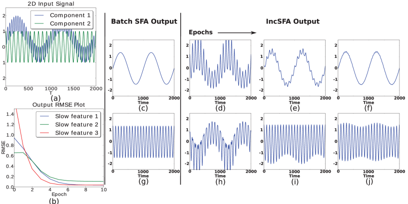
Figure 2: Experiment with a simple non-linear input signal. A learning rate of $\eta=0.08$ is used. (a) Input Signal (b) Output RMSE plot (c) Batch SFA output of the first slow feature (d)-(f) IncSFA output at t = 2, 5, 10 epochs. (g) Batch SFA output of the second slow feature (h)-(j) IncSFA output at t = 2, 5, 10 epochs.

As a basic proof of concept, IncSFA is applied to problem introduced in the original SFA paper (Wiskott and Sejnowski, 2002). The input signal is

$$\breve{x}_{1}(t) = \mbox{sin}(t)+\mbox{cos}(11~{}t)^{2},$$ (45)

$$\breve{x}_{2}(t) = \mbox{cos}(11~{}t),~{}t\in[0,2\pi],$$ (46)

Both vary quickly over time (see Figure 2(a)). A total of $2,000$ discrete datapoints are used for learning. The slowest feature hidden in the signal is $y_{1}(t)=\breve{x}_{1}(t)-\breve{x}_{2}(t)^{2}=\mbox{sin}(t)$, and the second is $\breve{x}_{2}(t)^{2}$.

Both BSFA and IncSFA extract these features. Figure 2(b) shows the Root Mean Square Error (RMSE) of IncSFA signals compared to the BSFA output, over multiple epochs of training. The RMSE at the end of 10 epochs is found to be equal to $[0.0360,0.1078,0.0377]^{T}$.

Figure 2(c) and (g) shows feature outputs of batch SFA, and (to the right) IncSFA outputs at $2,~{}5$, and $10$ epochs. Figures 2(g)-(j) show this comparison for the second feature.

This result show that it is indeed possible to extract multiple slow features in an online way without storing covariance matrices.

5.2 Extraction of a Driving Force from High Dimensional Input

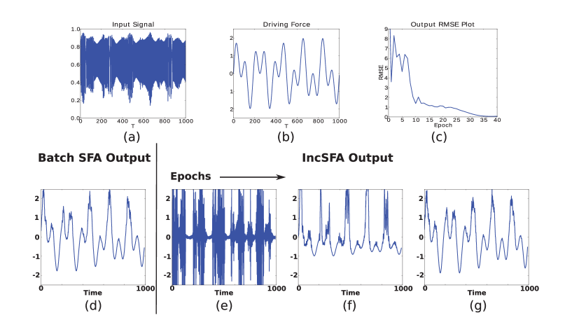
Figure 3: Experiment with a chaotic time series derived from a logistic map. A learning rate of $\eta=0.004$ is used. (a) Driving Force (b) Input (c) Output RMSE plot (d) BSFA output of the slowest feature (e)-(g) IncSFA output at t = 15, 30, 60 epochs.

A classic slow feature extraction problem involves uncovering the driving force of a dynamic system hidden in a very complex signal. Here, a chaotic time series is derived from a logistic map (T. Zito and Berkes, 2008):

$$\breve{x}(t+1)=(3.6+0.13~{}\gamma(t))\breve{x}(t)~{}(1-x(t)),$$ (47)

which is driven by a slowly varying driving force $\gamma(t)$ made up of two frequency components (5 and 11 Hz) given by

$$\gamma(t)=\mbox{sin}(10\pi t)+\mbox{sin}(22\pi t).$$ (48)

To show the complexity of the signal, figures 3(a) and 3(b) plot the driving force signal $\gamma(t)$ and the generated time series $\breve{x}(t)$, respectively.

A total of $1,000$ discrete datapoints are used. The driving force cannot be extracted linearly, so a nonlinear expansion is used—temporal in this case. The signal is embedded in 10 dimensional space using a sliding temporal window of size 10 (the TimeFramesNode from the MDP toolkit (T. Zito and Berkes, 2008) is used for this). The signal is then spatially quadratically expanded to generate an input signal with 65 dimensions.

Figure 3(c) shows the convergence of IncSFA on the BSFA output, Figure 3(d) BSFA output, and Figures 3(e)-(g) the outputs of IncSFA at 15, 30 and 60 epochs. The RMSE at $60^{th}$ epoch is found to be equal to $0.0984$.

5.3 Invariant Spatial Coding from Simple Movement Data

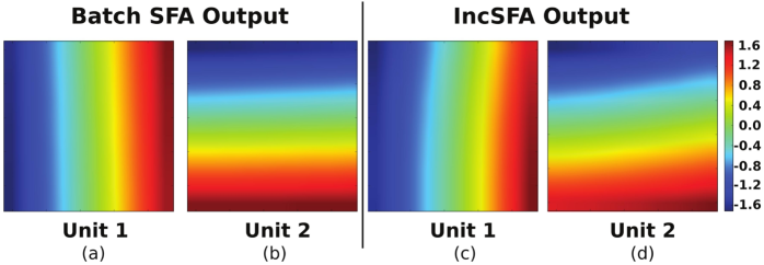
Figure 4: (a) BSFA output of the first slow feature and (b) the second slow feature (c) IncSFA output of the first slow feature and (d) the second slow feature after 50,000 samples with learning rate $\eta=0.003$ (figures best viewed in color).

Our simulated agent performs a random walk in a two-dimensional bounded space. Brownian motion is used to generate agent trajectories approximately like those of rats. The agent’s position $p(t)=[x(t),y(t)]$ is updated by a weighted sum of the current velocity and gaussian white noise, with standard deviation $v_{r}$. The momentum term $m$ can assume values between zero and one, so that higher values of $m$ lead to smoother trajectories and more homogeneous sampling of space in less time. Once the agent is predicted to cross the spatial boundaries, the current velocity is halved and an alternative random velocity update is generated, until a new valid position is reached. Noise variance $v_{r}=[3.0,2.5]^{T}$, mass $m=0.75$ and $50,000$ data points are used for generating the training set. A separate test grid dataset samples positions and orientations at regular intervals, and is used for evaluation.

Here is the used movement paradigm:
$~{}~{}currVel\leftarrow p(t)-p(t-1);\\ ~{}~{}\textbf{repeat}\\ ~{}~{}~{}~{}~{}noise\leftarrow GaussianWhiteNoise2d()*v_{r};\\ ~{}~{}~{}~{}~{}p(t+1)\leftarrow p(t)+m*currVel+(1-m)*noise;\\ ~{}~{}~{}~{}~{}\textbf{if}~{}not~{}isInsideWalkArea(p(t+1)):\\ ~{}~{}~{}~{}~{}~{}~{}~{}currVel\leftarrow currVel/2;\\ ~{}~{}\textbf{until}~{}isInsideWalkArea(p(t+1))\\$ Under this movement paradigm (Franzius et al., 2007), SFA yields slow feature outputs in the form of half-sinusoids, shown in Figure 4. These features collectively encode the agent’s $x$ and $y$ position in the environment. The first slow feature (Figure 4(a)) is invariant to the agent’s $x$ position, the second (Figure 4(b)) to its $y$ position ($y$ axis horizontal). IncSFA’s results (Figures 4(c)-(d)) are close to the ones of the batch version, with an RMSE of $[0.0536,0.0914]^{T}$.

5.4 Feature Adaptation to a Changing Environment

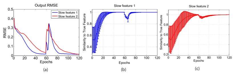
Figure 5: (a) RMSE of IncSFA’s first two output functions with respect to the true functions for original signal (epochs 1-59), and switched signal (epochs 60-120). (b) Normalized similarity (direction cosine) of the first slow feature to the true first slow feature of the current process, over 25 independent runs. (c) Normalized similarity of the second incremental slow feature.

The purpose of this experiment is to illustrate how IncSFA’s features adapt to a sudden shift in the input process. The input used is the same signal as in Experiment #1, but broken into two partitions. At epoch 60, the two input lines $x_{1}$ and $x_{2}$ are switched such that the $x_{1}$ signal suddenly carries what $x_{2}$ used to, and vice versa. We wish to show that IncSFA can first learn the slow features of the first partition, then is able to adapt to learn the slow features of the second partition.

The signal is sampled 500 times per epoch. The CCIPCA learning rate parameters, also used to set the learning rate of the input average $\bar{{\bf x}}$, were set to $t_{1}=20,t_{2}=200,c=4,r=5000$. The MCA learning rate is $\eta=0.01$.

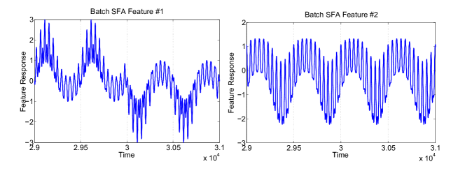
Figure 6: Outputs of first two slow features, from epoch 59 through 61, extracted by batch SFA over the input sequence.

Results of IncSFA are shown in Fig. 5, demonstrating successful adaptation. To measure convergence accuracy, we use the direction cosine (Chatterjee et al., 2000) between the estimated feature ${\bf w}(t)$ and true (unit length) feature ${\bf w}^{*}$,

$$DirectionCosine(t)=\displaystyle\frac{|{\bf w}^{T}(t)\cdot{\bf w}^{*}|}{\|{\bf w}^{T}(t)\|\cdot\|{\bf w}^{*}\|},$$ (49)

The direction cosine equals one when the directions align (the feature is correct) and zero when they are orthogonal.

BSFA results are shown in Fig. 6. The first batch feature catches the meta-dynamics and could actually be used to roughly sense the signal switch. However, the dynamics within each partition are not extracted.

5.5 Recovery from Outliers

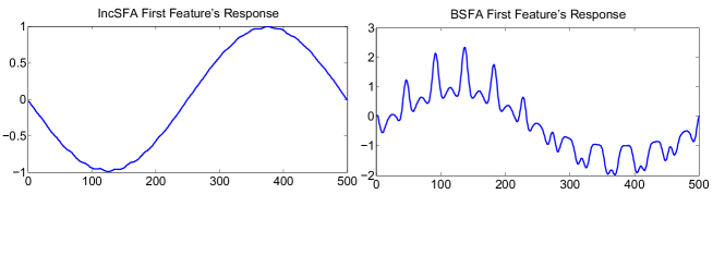
Figure 7: First output signals of IncSFA and BSFA on the simple signal with a single outlier.

Again, the learning rate setup and basic signal from the previous experiment is used, over 150 epochs, with 500 samples per epoch. A single outlier point is inserted: $x_{1}(100)=x_{2}(100)=2000$. Figure 7 shows the first output signal of BSFA and IncSFA, showing that the one outlier point at time 100 (out of 75,000) is enough to corrupt the first feature of BSFA, whereas IncSFA recovers.

The relative lack of sensitivity of IncSFA to outliers is shown in a real-world experiment (Kompella et al., 2011b), in which a person moves back and forth in front of a stable camera. At only one point in the training sequence, a door in the background is opened, and the BSFA hierarchical network’s first slow feature became sensitive to this event. Yet, the AutoIncSFA network’s first slow feature encodes the relative distance of the moving interactor.

5.6 High-Dimensional Video with Linear IncSFA

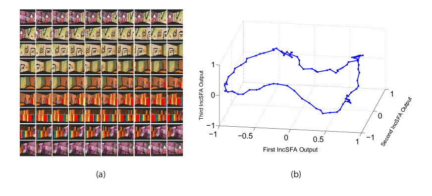
Figure 8: (a) Stream of 90 $41\times 41\times 3$ images as the agent completes one turn (360 degrees). Viewed row-wise, left to right. (b) Data projected onto the first three features learned by IncSFA. This gives a compact encoding of the agent’s state.

IncSFA’s scalability is tested with an image sequence of dimension $41\times 41\times 3$ (color images: see Fig. 8(a)). The agent is located in the middle of a square room with four complex-textured walls. In each episode, starting from a different orientation, the agent rotates slowly (4 degree shifts from one image to the next) by 360 degrees. At any time, a slight amount of Gaussian noise is added to the image ($\sigma=8$). The agent has a video input sensor, and the sequence of image frames with $5,043$ dimensions is fed into a linear IncSFA directly.

To reduce computation time, only the $40$ most significant principal components are computed by CCIPCA, using learning rate parameters $t_{1}=20,~{}t_{2}=200,~{}c=4,~{}r=5000$. Computation of the covariance matrix and its full eigendecomposition (including over 5000 eigenvectors and eigenvalues) is avoided. On the $40\times 40$ whitened difference space, only the first $5$ slow features are computed via MCA and sequential addition. $500$ epochs through the data took approximately 15 minutes using Matlab on a machine with an Intel i3 CPU and 4 GB RAM.

The result of projecting the (noise-free) data onto the first three slow features are shown in Fig. 8(b). A single linear IncSFA has incrementally compressed this high-dimensional noisy sequence to a nearly unambiguous compact form, learning to ignore the details at the pixel level and attend to the true cyclical nature underlying the image sequence. A few subsequences have somewhat ambiguous encodings, because certain images associated with slightly different angles are very similar.

5.7 High-Dimensional Video and Episodic Learning

“Real-world” learning systems might operate in series of several episodes of interactions with the environment. IncSFA can be readily extended to episodic tasks, with a minor modification: The derivative signal, which is computed as a difference over a single time step, is simply not computed for the starting sample of each episode. The first data point in each episode is used for updating the PCs, but not the slow feature vectors.

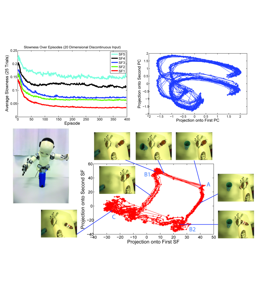
Figure 9: Experimental result of IncSFA on episodes where the iCub knocks down two cups via motor babbling on one joint. Upper left: The average slowness of the five features at each episode. Upper right: after training, several episodes (each episode is an image sequence where the cups are eventually both knocked down) are embedded in the space spanned by the first two PCs. Lower right: the same episodes are embedded in the space spanned by the first two slow features. We show some example images and where they lie in the embedding. The cluster in the upper right (A) represents when both cups are upright. When the robot knocks down the blue cup first, it moves to the cluster in the upper left (B1). If it instead knocks down the brown cup, it moves to the lower right cluster (B2). Once it knocks down both cups, it moves to the lower left area (C).

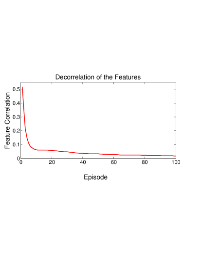
Figure 10: Average slow feature similarity over episodes.

Here we present results obtained through a robot’s episodic interactions with objects in its field of view. Two plastic cups are placed in the iCub robot’s field of view. The robot performs motor babbling in one joint using a movement paradigm of Franzius et al. During the course of babbling, it happens to topple the cups, in one of two possible orders. The episode ends a short time after it has knocked both down. A new episode begins with the cups upright again and the arm in the beginning position. A total of $50$ separate episodes were used as training data.

Linear IncSFA is used on the entire $80\times 60$ (grayscale) image. Only the $20$ most significant principal components are computed by CCIPCA, using learning rate parameters $t_{1}=20,~{}t_{2}=200,~{}c=2,~{}r=10000$. Only the first $5$ slow features are computed via MCA and sequential addition, with learning rate $0.001$. The MCA vectors are normalized after each update during the first $10$ epochs, but not thereafter (for faster convergence). Each of 25 different trials was over $400$ randomly-selected (of the 50 possible) episodes.

Results are shown in Fig. 9. We measured the slowness of the features on three “testing” episodes, after each episode of training. The upper left plot shows that all five features get slower over the episodes. After training completes, we can embed the data in a lower dimension with respect to the learned features. The embedding of 20 episodes are shown with respect to the first two PCs as well as the first two slow features. Since the cups being toppled or upright are the slow events in the scene, IncSFA’s encoding is keyed on the object’s state (toppled or upright). PCA does not find such an encoding, being much more sensitive to the arm. Since these events occurs once within each episode, BSFA cannot be used to learn these features. Figure 10 shows the average mutual direction cosine between non-identical pairs of slow features, and we can see the features quickly become nearly decorrelated.

Such clear object-specific low-dimensional encoding, invariant to the robot’s arm position, is useful, greatly facilitating training of a subsequent regressor or reinforcement learner. A video of the experimental result can be found at http://www.idsia.ch/~luciw/IncSFAArm/IncSFAArm.html.

5.8 Hierarchical IncSFA

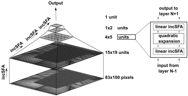
Figure 11: Example Hierarchical IncSFA Architecture, also showing the structure of an IncSFA node, which contains a linear IncSFA unit followed by nonlinear expansion followed by another linear IncSFA unit.

Deep networks composed of multiple stacked IncSFA nodes, each sensitive to only a small part of the input (i.e., receptive fields), can be used for processing high-dimensional image streams in a biologically plausible way. The computational reason for doing this is that very high-dimensional signals correspond to large search spaces, and hierarchical setups breaking up the signal can reduce the search burden. And using receptive fields reduces the number of necessary lower-order PCs that have to be computed by CCIPCA, which should speed the learning.

Figure 11 shows an example deep network, motivated by the human visual system and based on the one specified by Franzius et al. (Franzius et al., 2007). The network is made up of a converging hierarchy of layers of IncSFA nodes, with overlapping rectangular receptive fields. Each IncSFA node finds the slowest output features from its input within the subspace of all monomials (e.g., of degree two if a quadratic expansion is used) of the node’s inputs.

We feed IncSFA with images from a high-dimensional video stream generated by the iCub simulator (V. Tikhanoff and Nori, 2008), an OpenGL-based software specifically built for the iCub robot. Our experiment mimics the robot observing a moving interactor agent, which in the simulation takes the form of a rectangular flat board moving back and forth in depth over the range $[1,3]$ (meters) in front of the robot, using a movement paradigm similar to the one discussed in Section 5.3. Figure 12(a) shows the experimental setup in the iCub simulator. Figure 12(b) shows a sample image from the dataset. $20,000$ monocular images are captured from the robot’s left eye and downsampled to 83$\times$100 pixels (input dimension of $8,300$).

A three-layer IncSFA network is used to encode the images. Each SFA node operates on a spatial receptive field of the layer below. The first layer uses $15\times 19$ nodes, each with $10\times 10$ image patch receptive field and a $5$ pixel overlap. Each node on this layer develops 10 slow features. The second layer uses $4\times 5$ nodes, each having a $5\times 5$ receptive field, and developing 5 slow features. The third layer uses two nodes, one sensitive to the top half, the other sensitive to the bottom half (5 slow features). The forth layer uses a single node and a single slow feature. The network is trained layer-wise from bottom to top, with the lower layers frozen once a new layer begins its training. The CCIPCA output of all nodes is clipped to $[-5,5]$, to avoid any outliers that may arise due to close-to-zero eigenvalues in some of the receptive fields that contain unchanging stimuli. Each IncSFA node is trained individually, that is, there is no weight sharing among nodes.

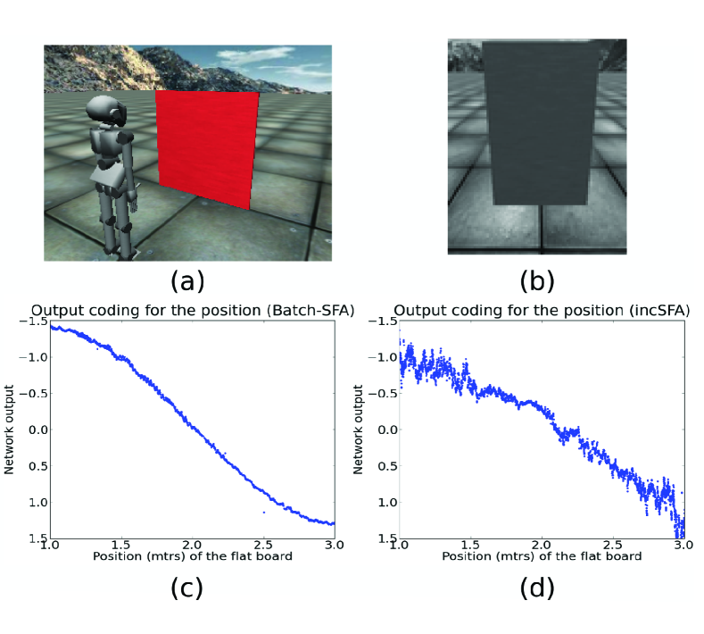
Figure 12: (a) Experimental Setup: iCub Simulator (b) Sample image from the input dataset (c) Batch-SFA output (d) IncSFA output ($\eta=0.005$)

For comparison, a batch SFA hierarchical network was also trained on this data. Figures 12 show BSFA and IncSFA outputs. The expected output is of the form of a sinusoid extending over the range of board positions. IncSFA gives a slightly noisy output, probably due to the constant dimensionality reduction value for all units in each layer of the network, selected to maintain a consistent input structure for the subsequent layer; hence some units with eigenvectors corresponding to very small eigenvalues emerge in the first stage, with receptive fields observing comparatively few input changes, thus slightly corrupting the whitening result, and adding small fluctuations to the overall result.

Finally, we evaluate how well the IncSFA feature codes for distance. A supervised quadratic regressor is trained with ground truth labels on 20% of the dataset, and tested on the other 80%, to measure the quality of features for some classifier or reinforcement learner using them (see RMSE plot). Hierarchical IncSFA derives the driving forces from a complex and continuous input video stream in a completely online and unsupervised manner.

6 Conclusions

Our novel Incremental Slow Feature Analysis technique solves SFA problems incrementally without storing covariance matrices. IncSFA’s covariance-free Hebbian and anti-Hebbian updates add biological plausibility to SFA itself. While batch SFA cannot handle certain open-ended uncontrolled settings, IncSFA can. This makes it a promising tool for learning autonomous robots. Future work will study online learning controllers whose experiments actively create data exhibiting novel but learnable regularities measured by improvements of emerging slow features, in line with the formal theory of curiosity (Schmidhuber, 2010).

Acknowledgments

The experimental paradigm used for the distance-encoding high-dimensional video experiment was first developed by the first author under the supervision of Mathias Franzius, at the Honda Research Institute Europe. We would like to acknowledge Dr. Franzius for his contributions in this regard. We would also like to acknowledge IDSIA researchers Alexander Forster and Kail Frank for enabling the experiment with the iCub robot. Thanks to Marijn Stollenga and Sohrob Kazerounian for their comments on an earlier draft of the paper. This work was funded through the 7th framework program of the EU under grants #231722 (IM-Clever project) and #270247 (NeuralDynamics project), and by Swiss National Science Foundation grant CRSIKO-122697 (Sinergia project).

References

- Abut (1990) Abut, H., editor (1990). Vector Quantization. IEEE Press, Piscataway, NJ.
- Amari (1977) Amari, S. (1977). Neural theory of association and concept-formation. Biological Cybernetics, 26(3):175–185.
- Barlow (2001) Barlow, H. (2001). Redundancy reduction revisited. Network: Computation in Neural Systems, 12(3):241–253.
- Bergstra and Bengio (2009) Bergstra, J. and Bengio, Y. (2009). Slow, decorrelated features for pretraining complex cell-like networks. Advances in Neural Information Processing Systems 22, pages 99–107.
- Chatterjee et al. (2000) Chatterjee, C., Kang, Z., and Roychowdhury, V. (2000). Algorithms for accelerated convergence of adaptive pca. IEEE Transactions on Neural Networks, 11(2):338–355.
- Chen et al. (1998) Chen, T., Amari, S., and Lin, Q. (1998). A unified algorithm for principal and minor components extraction. Neural Networks, 11(3):385–390.
- Chen et al. (2001) Chen, T., Amari, S., and Murata, N. (2001). Sequential extraction of minor components. Neural Processing Letters, 13(3):195–201.
- Comon (1994) Comon, P. (1994). Independent component analysis, A new concept? Signal Processing, 36:287–314.
- Dayan and Abbott (2001) Dayan, P. and Abbott, L. (2001). Theoretical neuroscience: Computational and mathematical modeling of neural systems.
- (10) Doersch, C., Lee, T., Huang, G., and Miller, E. Temporal continuity learning for convolutional deep belief networks.
- Földiák (1991) Földiák, P. (1991). Learning invariance from transformation sequences. Neural Computation, 3(2):194–200.
- Franzius et al. (2007) Franzius, M., Sprekeler, H., and Wiskott, L. (2007). Slowness and sparseness lead to place, head-direction, and spatial-view cells. PLoS Computational Biology, 3(8):e166.
- Gisslen et al. (2011) Gisslen, L., Luciw, M., Graziano, V., and Schmidhuber, J. (2011). Sequential constant size compressors for reinforcement learning. In Fourth Conference on Artificial General Intelligence (AGI).
- Grossberg (1980) Grossberg, S. (1980). How does a brain build a cognitive code?. Psychological Review, 87(1):1.
- Hafting et al. (2005) Hafting, T., Fyhn, M., Molden, S., Moser, M., and Moser, E. (2005). Microstructure of a spatial map in the entorhinal cortex. Nature, 7052:801.
- Hinton (1989) Hinton, G. (1989). Connectionist learning procedures. Artificial Intelligence, 40(1-3):185–234.
- Hinton (2002) Hinton, G. E. (2002). Training products of experts by minimizing contrastive divergence. Neural Comp., 14(8):1771–1800.
- Jenkins and Matarić (2004) Jenkins, O. and Matarić, M. (2004). A spatio-temporal extension to isomap nonlinear dimension reduction. In Proceedings of the twenty-first international conference on Machine learning, page 56. ACM.
- Jolliffe (1986) Jolliffe, I. T. (1986). Principal Component Analysis. Springer-Verlag, New York.
- Klapper-Rybicka et al. (2001) Klapper-Rybicka, M., Schraudolph, N. N., and Schmidhuber, J. (2001). Unsupervised learning in LSTM recurrent neural networks. In Lecture Notes on Comp. Sci. 2130, Proc. Intl. Conf. on Artificial Neural Networks (ICANN-2001), pages 684–691. Springer: Berlin, Heidelberg.
- Kohonen (2001) Kohonen, T. (2001). Self-Organizing Maps. Springer-Verlag, Berlin, 3rd edition.
- Kompella et al. (2011a) Kompella, V., Luciw, M., and Schmidhuber, J. (2011a). Incremental slow feature analysis. In International Joint Conference of Artificial Intelligence.
- Kompella et al. (2011b) Kompella, V. R., Pape, L., Masci, J., Frank, M., and Schmidhuber, J. (2011b). Autoincsfa and vision-based developmental learning for humanoid robots. In IEEE-RAS International Conference on Humanoid Robots, Bled, Slovenia.
- Krasulina (1970) Krasulina, T. (1970). Method of stochastic approximation in the determination of the largest eigenvalue of the mathematical expectation of random matrices. Automat. Remote Contr, 2:215–221.
- Kreyszig (1988) Kreyszig, E. (1988). Advanced engineering mathematics. Wiley, New York.
- Lee and Seung (1999) Lee, D. and Seung, H. (1999). Learning the parts of objects by non-negative matrix factorization. Nature, 401(6755):788–791.
- Lee et al. (2010) Lee, H., Largman, Y., Pham, P., and Ng, A. (2010). Unsupervised feature learning for audio classification using convolutional deep belief networks. Advances in neural information processing systems, 22:1096–1104.
- Legenstein et al. (2010) Legenstein, R., Wilbert, N., and Wiskott, L. (2010). Reinforcement learning on slow features of high-dimensional input streams. PLoS Computational Biology, 6(8).
- Lindstädt (1993) Lindstädt, S. (1993). Comparison of two unsupervised neural network models for redundancy reduction. In Mozer, M. C., Smolensky, P., Touretzky, D. S., Elman, J. L., and Weigend, A. S., editors, Proc. of the 1993 Connectionist Models Summer School, pages 308–315. Hillsdale, NJ: Erlbaum Associates.
- Mitchison (1991) Mitchison, G. (1991). Removing time variation with the anti-hebbian differential synapse. Neural Computation, 3(3):312–320.
- Oja (1982) Oja, E. (1982). Simplified neuron model as a principal component analyzer. Journal of mathematical biology, 15(3):267–273.
- Oja (1985) Oja, E. (1985). On stochastic approximation of the eigenvectors and eigenvalues of the expectation of a random matrix. Journal of Mathematical Analysis and Applications, 106:69–84.
- Oja (1992) Oja, E. (1992). Principal components, minor components, and linear neural networks. Neural Networks, 5(6):927–935.
- O’Keefe and Dostrovsky (1971) O’Keefe, J. and Dostrovsky, J. (1971). The hippocampus as a spatial map: Preliminary evidence from unit activity in the freely-moving rat. Brain research.
- Papoulis et al. (1965) Papoulis, A., Pillai, S., and Unnikrishna, S. (1965). Probability, random variables, and stochastic processes, volume 196. McGraw-hill New York.
- Peng and Yi (2006) Peng, D. and Yi, Z. (2006). A new algorithm for sequential minor component analysis. International Journal of Computational Intelligence Research, 2(2):207–215.
- Peng et al. (2007) Peng, D., Yi, Z., and Luo, W. (2007). Convergence analysis of a simple minor component analysis algorithm. Neural Networks, 20(7):842–850.
- Rolls (1999) Rolls, E. (1999). Spatial view cells and the representation of place in the primate hippocampus. Hippocampus, 9(4):467–480.
- Sanger (1989) Sanger, T. (1989). Optimal unsupervised learning in a single-layer linear feedforward neural network. Neural networks, 2(6):459–473.
- Schmidhuber (1992a) Schmidhuber, J. (1992a). Learning complex, extended sequences using the principle of history compression. Neural Computation, 4(2):234–242.
- Schmidhuber (1992b) Schmidhuber, J. (1992b). Learning factorial codes by predictability minimization. Neural Computation, 4(6):863–879.
- Schmidhuber (1992c) Schmidhuber, J. (1992c). Learning unambiguous reduced sequence descriptions. In Moody, J. E., Hanson, S. J., and Lippman, R. P., editors, Advances in Neural Information Processing Systems 4 (NIPS 4), pages 291–298. Morgan Kaufmann.
- Schmidhuber (1999) Schmidhuber, J. (1999). Neural predictors for detecting and removing redundant information. In Cruse, H., Dean, J., and Ritter, H., editors, Adaptive Behavior and Learning. Kluwer.
- Schmidhuber (2010) Schmidhuber, J. (2010). Formal theory of creativity, fun, and intrinsic motivation (1990–2010). IEEE Transactions on Autonomous Mental Development, 2(3):230–247.
- Sprekeler et al. (2010) Sprekeler, H., Zito, T., and Wiskott, L. (2010). An extension of slow feature analysis for nonlinear blind source separation.
- T. Zito and Berkes (2008) T. Zito, N. Wilbert, L. W. and Berkes, P. (2008). Modular toolkit for data processing (mdp): a python data processing framework. Frontiers in Neuroinformatics, 2.
- Taube et al. (1990) Taube, J., Muller, R., and Ranck, J. (1990). Head-direction cells recorded from the postsubiculum in freely moving rats. i. description and quantitative analysis. The Journal of Neuroscience, 10(2):420.
- V. Tikhanoff and Nori (2008) V. Tikhanoff, A. Cangelosi, P. F. G. M. L. N. and Nori, F. (2008). An open-source simulator for cognitive robotics research: The prototype of the icub humanoid robot simulator.
- Wang and Karhunen (1996) Wang, L. and Karhunen, J. (1996). A unified neural bigradient algorithm for robust pca and mca. International journal of neural systems, 7(1):53.
- Weng and Zhang (2006) Weng, J. and Zhang, N. (2006). Optimal in-place learning and the lobe component analysis. In Neural Networks, 2006. IJCNN’06. International Joint Conference on, pages 3887–3894. IEEE.
- Weng et al. (2003) Weng, J., Zhang, Y., and Hwang, W. (2003). Candid covariance-free incremental principal component analysis. 25(8):1034–1040.
- Wiskott (2003) Wiskott, L. (2003). Estimating driving forces of nonstationary time series with slow feature analysis. Arxiv preprint cond-mat/0312317.
- Wiskott et al. (2011) Wiskott, L., Berkes, P., Franzius, M., Sprekeler, H., and Wilbert, N. (2011). Slow feature analysis. Scholarpedia, 6(4):5282.
- Wiskott and Sejnowski (2002) Wiskott, L. and Sejnowski, T. (2002). Slow feature analysis: Unsupervised learning of invariances. Neural Computation, 14(4):715–770.
- Xu et al. (1992) Xu, L., Oja, E., and Suen, C. (1992). Modified hebbian learning for curve and surface fitting. Neural Networks, 5(3):441–457.
- Zhang and Weng (2001) Zhang, Y. and Weng, J. (2001). Convergence analysis of complementary candid incremental principal component analysis. Michigan State University.