Extreme events and event size fluctuations in biased random walks on networks

Abstract

Random walk on discrete lattice models is important to understand various types of transport processes. The extreme events, defined as exceedences of the flux of walkers above a prescribed threshold, have been studied recently in the context of complex networks. This was motivated by the occurrence of rare events such as traffic jams, floods, and power black-outs which take place on networks. In this work, we study extreme events in a generalized random walk model in which the walk is preferentially biased by the network topology. The walkers preferentially choose to hop toward the hubs or small degree nodes. In this setting, we show that extremely large fluctuations in event-sizes are possible on small degree nodes when the walkers are biased toward the hubs. In particular, we obtain the distribution of event-sizes on the network. Further, the probability for the occurrence of extreme events on any node in the network depends on its ’generalized strength’, a measure of the ability of a node to attract walkers. The ’generalized strength’ is a function of the degree of the node and that of its nearest neighbors. We obtain analytical and simulation results for the probability of occurrence of extreme events on the nodes of a network using a generalized random walk model. The result reveals that the nodes with a larger value of ’generalized strength’, on average, display lower probability for the occurrence of extreme events compared to the nodes with lower values of ’generalized strength’.

I Introduction

Extreme events are typically associated with disasters of some kind or other, e.g., droughts, cold wave, cyclones, earthquakes, wind gusts and economic recession. When a relevant variable, such as the wind speed $w(t)$ recorded at time $t$ in the case of wind gusts, exceeds certain prescribed threshold $q$ due to its inherent fluctuations, i.e., $w(t)>q$, then it is taken to be an extreme event. In particular, it is important to note that the magnitude of tremor, wind speed, temperature, economic growth etc. are scalar variables. A large number of results, both theoretical and empirical, are known about the statistics and dynamics of extreme events for such univariate, scalar variables eevent1 . One significant result due to classical extreme value theory is that, depending on the probability distribution function of the variable, the distribution of block maxima, for the uncorrelated sequence of random variables, converges to only one of the three possible forms, namely, Fréchet, Gumbel and Weibull distributions coles .

In contrast to this scenario, extreme events can also take place on complex networks. Consider, for instance, the most common experience of web surfers; a web server not responding due to the heavy load of http requests. This is an extreme event taking place on the network of world wide web. For example, the popular social networking site Twitter handled about 600 tweets per second in early 2010 tweet . According to an industry estimate, the Google search engine received approximately 34000 search requests per second by the end of 2009 google . For most websites on the world wide web that are unprepared for such a large number of http requests, these numbers would represent extreme events and could potentially disrupt the service. The power black-out in the north eastern United States in 2003 is also an example of extreme event on the power transmission grid network. The cascading failures shut down more than 508 power generating units at 265 power plants during the peak of this black-outblackout . Grid locks in highways is an example of extreme event on transportation network. From the point of view of physics, all these events could be thought of as an emergent phenomena arising due to flux on the networks and could be regarded as extreme events arising primarily due to limited handling capacity of the node. Transport on the networks continues to be widely studied but much less attention has been focused on it from the point of view of extreme events. Generally, when the flux (packets of information or power or highway traffic, in the case of examples given above) exceeds the handling capacity, it turns out to be an extreme event for the particular node on the network. In the earlier works related to congestion and cascade on networks congest1 ; congest2 ; congest3 ; congest4 ; congest5 ; congest6 ; congest7 ; congest8 , handling capacity is a key ingredient that needs to be prescribed upfront.

However, extreme events happen not only because of the limited handling capacity of the node on a network but also because of inherent fluctuations in the flux passing through the node. These fluctuations in the flux passing through a node could be so large as they breach a prescribed threshold, in which case, we label the event as an extreme event for the node. This definition of extreme event for a node on any network is similar in spirit to that of the classical extreme value theory. Then, a relevant question is how the connectivity of the network affects the probability for extreme event occurrence. By modeling the transport as standard random walks on networks, it was shown in Ref. vsa that the probability for the occurrence of extreme events $P(k_{i})$, arising due to inherent fluctuations, depends only on the degree $k_{i}$ of the $i$-th node in question. In this work, the threshold $q_{i}$ was chosen to be proportional to typical fluctuation size on $i$-th node. Thus, the extreme events are identified after taking care of the natural variability of the flux passing through the given node. Further, it was shown that, on average $P(k)$ is higher for small degree nodes than for hubs. This is a surprising result because it implies that, within the framework of random walk on networks, even though hubs attract large flux (compared to small degree nodes) they are less prone to extreme events. Thus, in the context of a node on a connected network, larger flux does not necessarily translate into higher probabilities for extreme events. This feature is one possible signature of connectivity, i.e., the network setting on which the system operates. In contrast, for a scalar time series $w(t)$ larger flux would imply higher extreme event probabilities.

Random walk on complex networks is a useful fundamental model against which to compare other transport processes. Most realistic transport phenomena on networks, such as the flux of information packets passing through the network of routers or road traffic, do not proceed by performing random walk. In order to model the flux in a more realistic way, it is useful to generalize the standard random walk to a situation in which the flux is either biased toward hubs or small degree nodes. For example, consider the case of two remote airports which are not directly connected by flights. Typically, they would be connected through a major hub on the airline network. This is one practical scenario in which the traffic is biased toward the hubs. This happens in many a network settings; railways tend to connect the hinterland with the hubs, phones connect to nearest hubs on the network. Motivated by these physical examples, in this work, we model the transport process as random walks biased by the topology of the network and study the extreme event probabilities and event-size distributions. We show that biased random walk leads to extreme fluctuations in the event sizes on the network. In the subsequent sections, we discuss the topologically biased random walk model on a network and obtain analytical results for the probability of occurrence of extreme events on any node. We show that the analytical and simulation results are in good agreement.

II Biased random walk on networks

II.1 Stationary distribution

We consider a connected, undirected, finite network with $N$ nodes and $E$ edges. The network is characterized by a symmetric adjacency matrix ${\mathbf{A}}$ with elements $A_{ij}=1$ if nodes $i$ and $j$ are connected by an edge and $A_{ij}=0$ otherwise. There are $W$ independent walkers performing biased random walk on this network in the sense explained below. We denote by $b_{ij}$ the transition probability for a walker to hop from node $i$ to a neighboring node $j$. Let $P_{ij}$ be the probability that a walker starting at the node $i$ at time $n=0$ is at node $j$ at time $n$. Then, the master equation can be written as

$$P_{ij}(n+1)=\sum_{l}A_{lj}~{}b_{lj}~{}P_{il}(n).$$ (1)

The random walkers are biased by taking the time-independent transition probability for hopping from $l$-th to $j$-th node to be fronczak1 ; fronczak2 ; yang

$$b_{lj}\propto k_{j}^{\alpha},$$ (2)

where $\alpha$ is a parameter that defines the degree of bias imparted to the walkers. Clearly, $\alpha=0$ corresponds to the standard random walk and the transition probability is unbiased, where the walker can hop to any of the neighboring node with equal probability. For $\alpha>0$, the random walkers are biased toward nodes with larger degree or hubs. In contrast, if $\alpha<0$, walkers preferentially hop to small degree nodes. The larger (smaller) the $\alpha$, stronger the bias toward the hubs (small degree nodes) is. Then, the normalized transition probability becomes

$$b_{lj}=\frac{k_{j}^{\alpha}}{\sum_{m=1}^{k_{l}}k_{m}^{\alpha}}.$$ (3)

The summation in the denominator runs over the nearest neighbors of node $l$. Using the transition probability in Eq.3, the master equation becomes

$$P_{ij}(n+1)=\sum_{l}A_{lj}\frac{k_{j}^{\alpha}}{\sum_{m=1}^{k_{l}}k_{m}^{\alpha}}P_{il}(n).$$ (4)

By repeated iteration of Eq. 4, it can be shown that $P_{ij}(n)$, as $n\to\infty$ leads to the stationary distribution

$$\lim_{n\to\infty}P_{ij}(n)=p_{j}=\frac{k_{j}^{\alpha}\sum_{l=1}^{k_{j}}k_{l}^{\alpha}}{\sum_{m=1}^{N}\left(k_{m}^{\alpha}\sum_{l=1}^{k_{m}}k_{l}^{\alpha}\right)}.$$ (5)

We can define the generalized strength of $j$ th node to be

$$\phi_{j}=k_{j}^{\alpha}{\sum_{i=1}^{k_{j}}k_{i}^{\alpha}},$$ (6)

which is a measure of the ability of a node to attract walkers. Note that $\phi_{j}$ depends on the bias parameter $\alpha$ and the degree of the nearest neighbors to which it is connected by an edge. Hence, it is possible for the nodes with same degree to have different generalized strengths. Thus, the generalized strength of the node is independent of the global network structure but is dependent on the local connectivity structure around the node. This is in contrast to the case of standard random walk (on networks) in which large-scale structure of the network topology plays no significant role. The local network structure is important for biased random walks on networks. In Fig. 1, we show how the generalized strength $\phi$ depends on the degree of a node, for several values of $\alpha$, in a scale-free network with degree exponent $\gamma=2.2$. For $\alpha=1$ (crosses in Fig. 1), the generalized strength of a node is higher for large degree nodes (hubs) and an approximate linear relation is seen between $\phi_{i}$ and $k_{i}$ of $i$-th node. For $\alpha=0$, which is the standard random walk case, the generalized strength of the node is the same as the degree of the node (solid circles in Fig. 1). However, for $\alpha=-1.0$, $\phi$ is independent of $k$ especially for large degree nodes (triangles in Fig. 1). In this case, the bias in the random walk represented by its generalized strength $\phi$ is balanced by the degree of the node. In a scale-free network, a large number of small degree nodes are present and they do not have identical values for the generalized strength $\phi$. This explains the spread in $\phi$ for all values for $k<50$. Upon further decrease in the bias parameter $\alpha$ below -1.0 (open squares in Fig. 1), nodes with a smaller degree or neighbors with smaller degree become important and the generalized strength decreases with increasing degree.

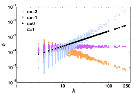
Figure 1: (Color online) Strength $\phi$ as a function of degree $k$ for different values of $\alpha$ in log-log plot.

II.2 Extreme event probability

The stationary distribution for the number of walkers in $j$-th node can be rewritten in terms of the generalized strength $\phi$ as

$$p_{j}=\frac{\phi_{j}}{\sum_{l=1}^{N}\phi_{l}}.$$ (7)

Thus, every node can be uniquely characterized by its generalized strength $\phi$. It is expected that two nodes with the same value of $\phi$ show similar behavior as far as biased walks on networks based on Eq. 2 are concerned. In case of $\alpha=0$, we get $\phi_{i}=k_{i}$ and the stationary distribution simplifies to $p_{j}=\frac{k_{j}}{2E}$, the result obtained for the case of standard random walk in Ref. rw1 . Thus, in the case of a standard random walk, the degree $k$ characterises the node. In the case of uncorrelated random networks, the stationary occupation probability can be further simplified by using the mean field approximation and can be written as fronczak1 ; fronczak2

$$p_{j}=\frac{k_{j}^{\alpha+1}}{N\langle k^{\alpha+1}\rangle}.$$ (8)

This approximate result suggests that the nodes with the same degree should have the identical transition probabilities fronczak1 . This does not necessarily hold well for the nodes of correlated networks such as the scale-free networks. This is because in a scale-free network, the neighbourhood of nodes with identical degree are not identical. Hence, to study extreme events we use Eq. 7 instead of Eq. 8.

Given that Eq. 7 gives the probability to find one walker on $i$-th node with generalized strength $\phi_{i}$, we can now obtain the distribution of random walkers on $i$-th node. The formulation is applicable to any node on the network and hence, in our further discussions, we suppress the index $i$ of the node. Random walkers are independent and non-interacting and hence the probability $f(w)$ of finding $w$ walkers on a node is $p^{w}$ while the rest of the walkers, $W-w$ are distributed on the rest of the nodes of the network. When properly normalized, this leads to a binomial distribution given by

$$f(w)={W\choose w}~{}p^{w}~{}(1-p)^{W-w}.$$ (9)

The mean and variance of the flux passing through the given node is

$$\langle f\rangle = W\frac{\phi}{\sum_{l=1}^{N}\phi_{l}},$$

$$\sigma^{2} = W\frac{\phi}{\sum_{l=1}^{N}\phi_{l}}\left(1-\frac{\phi}{\sum_{l=1}^{N}\phi_{l}}\right).$$ (10)

Note that the results in Eqs. 9 and 10 depend only on the generalized strength $\phi$ that characterises a node including its neighbourhood. It does not depend on the large scale connectivity pattern. Hence, these results will hold good for any network, such as scale-free, random or small world, irrespective of its degree distribution. Further, in the cases for which $\sum_{l=1}^{N}\phi_{l}>>\phi$, we obtain the approximate relation $\sigma\approx\langle f\rangle^{1/2}$. This relation can be thought of as a generalization of a similar relation for the unbiased random walks reported in Ref. vsa . However, the exponent $1/2$ is not universal and instead depends on details such as the fluctuation in number of walkers and sampling resolution of the flux breakdown . The distribution of random walkers on two nodes with different degrees, $k=4$ and $k=234$, is plotted in Fig. 2. The biased random walk simulations were performed on a scale-free network with 5000 nodes with 19915 links and 39830 walkers. Initially, at time $n=0$, the walkers are randomly distributed on $N$ nodes. The simulation results presented in Fig. 2 have been obtained after averaging over 100 realisations with different initial conditions of random walkers. The simulation results, the solid lines in Fig. 2, show a good agreement with the analytical distribution given by Eq. 9.

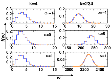
Figure 2: (Color online) The distribution of walkers on two nodes with $k=4$ and $k=234$ for ${\alpha}=-1.0,0.0$ and $1.0$. The solid lines show the distribution of walkers obtained from simulation while solid circles belong to the binomial distribution obtained analytically using the stationary probability in Eq. (7).

III Probability for extreme events

We take an extreme event to be the one for which the probability of occurrence is small and is typically associated with the tail of the probability distribution function for the events. We extend this principle to the events on the nodes of a network vsa . Given that the number of walkers $w$ passing through a node with generalized strength $\phi$ follow the Binomial distribution, if more than $q$ walkers pass through the node, then it is an extreme event for the node. Then, the probability for the occurrence of extreme event is

$$F_{i} = \sum_{w=q_{i}}^{W}~{}{W\choose w}~{}{p}_{i}^{w}~{}(1-{p}_{i})^{W-w},$$ (11)

$$= I_{p_{i}}(\lfloor q_{i}\rfloor+1,W-\lfloor q_{i}\rfloor),$$ (12)

where $\lfloor u\rfloor$ is the floor function defined as the largest integer not greater than $u$ and $I_{z}(a,b)$ is the standard incomplete Beta function lopez . In this form, the extreme event probability will depend on the choice of threshold $q_{i}$. First, we consider the case of constant threshold. If $q_{i}=0$, using Eq. 11 we obtain $F_{i}=1$ for all the nodes on the network. Thus, all the nodes will experience extreme events all the time. On the other hand, if we set $q_{i}=W$, then we obtain

$$F_{i}=p_{i}^{W}.$$ (13)

Since $p_{i}<<1$, we get $F_{i}\approx 0$ for all the nodes implying that there are no extreme events anywhere in the network. Hence, these choices of threshold values are not physically interesting cases. Any other arbitrary choice such as $q_{i}=q_{0}$, where $q_{0}$ is a constant, will predominantly lead to some nodes encountering extreme events nearly all the time and others having no events at all. This too is not an interesting case. The foregoing arguments imply that an interesting scenario would arise if the threshold is chosen to be proportional to the natural variability of the flux passing through a node. Thus, we choose the threshold for extreme events to be vsa

$$q_{i}=\langle f_{i}\rangle+m\sigma_{i},$$ (14)

where $m\geq 0$. The mean flux $\langle f_{i}\rangle$ and standard deviation $\sigma_{i}$ are given by Eq. 10. Substituting $q_{i}$ in Eq. 12, it is clear that the probability for the occurrence of extreme events is dependent only on the generalized strength $\phi$ of the node. In Fig. 3, we show the simulation and analytical results for the probability of extreme events as a function of $\phi$ for several choices of $\alpha$. The numerical results are based on simulations with $W=39380$ walkers on a scale-free network with $N=5000$ nodes evolved for $10^{7}$ time steps. An unusual feature is that $F_{i}$ predicts higher probability of occurrence of extreme events, on average, for nodes with small values of generalized strength $\phi$ than for the nodes with higher values of generalized strength $\phi$. For instance, in Fig. 3(a), the probability of extreme event occurrence is generally higher for nodes with $\phi<10^{-5}$ than for nodes with $\phi>10^{-3}$. A similar effect is seen in Figs. 3(b)- 3 (e). Even though nodes with higher the generalized strength $\phi$ attract more walkers as given by Eq. 5, this does not imply that they also have higher probability for extreme events. This is a generalization of the result obtained in Ref. vsa for the standard random walk on networks which shows that the extreme events are more probable for nodes with small degree than for the ones with high degree. The local fluctuations seen in Fig. 3 are inherent in the system and not due to insufficient ensemble averaging. Further, notice that Eq. 12 does not depend on the large scale structure of the topology and hence it is valid for biased random walks on any topology, random or small-world or scale-free.

However, the local connectivity patterns in the vicinity of any node plays a crucial role in the diffusion of an extreme event. Suppose an extreme event takes place at node $A$ at time $n$, then one interesting question is how probable it is for an extreme event to take place in its immediate neighborhood at time $n+1$, i.e, after the first jump. We call it first-jump probability and it is similar to the one reported in arw1 . In the case of a standard random walk ($\alpha=0$), our simulations (not shown here) indicate that in general if node $A$ is a hub, then the probability to encounter an extreme event in its neighbourhood is higher (at least by a factor of 3-4) compared to the case when node $A$ is a small degree node. For biased random walks, the results suggest a higher likelihood for an extreme event to be transferred to its neighbourhood in the case when $\alpha<0$ compared to the case with $\alpha>0$.

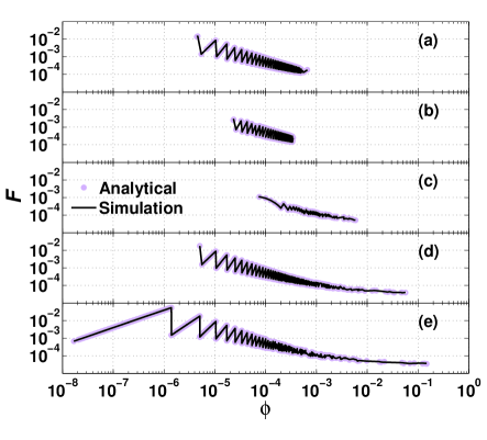
Figure 3: (Color online) The probability for the occurrence of extreme events plotted as a function of node generalized strength $\phi$ (normalized) for different values of bias parameters (a) $\alpha=-2.0$, (b) $\alpha=-1.0$, (c) $\alpha=0.0$, (d) $\alpha=1.0$ and (e) $\alpha=2.0$. The threshold for extreme event is $q=\langle f\rangle+4\sigma$. The circles are from analytical results in Eq. (12) while solid lines are the simulation results performed on a scale-free network ($N=5000$, $E=19915$) with $W=2E$ walkers averaged over 100 realizations with randomly chosen initial positions of walkers.

IV Fluctuations in event size

The size of an event is measured in units of the standard deviation $\sigma$ of the flux passing through a node. In this section, we show that the extreme fluctuations in the flux of walkers are realised in the case of $\alpha=2$ which implies that the walkers are biased toward the nodes with larger generalised strength $\phi$ (hubs). An event is of size $m$ if $m\sigma\leq w-\langle w\rangle<(m+1)\sigma$, where $w$ is the number of walkers on a given node.

Then, the probability for the occurrence of an event of size $m$ can be written down as,

$$\mathcal{P}_{m}=I_{p}(\lfloor q_{m}\rfloor+1,W-\lfloor q_{m}\rfloor)-I_{p}(\lfloor q_{m+1}\rfloor+1,W-\lfloor q_{m+1}\rfloor).$$ (15)

To illustrate the result, we show the distribution of event sizes in Fig. 4 for $\alpha=-2,-1,0,1,2$ in a scale-free network obtained from simulations evolved for $10^{7}$ steps and averaged over $100$ ensembles. Here, the events with probability of occurrence of less than $10^{-8}$ have been discarded to maintain the numerical accuracy. In the case of $\alpha=0$ (standard random walk), the distribution of events is shown in Fig. 4(c). The events of size $m=0$ are highly probable with $\mathcal{P}_{0}\sim 0.1$. In contrast, the probability for the events of size $|m|>0$ decrease and thus the extreme events of size $m=-2,8$ occur with probability $\mathcal{P}_{-2}\sim\mathcal{P}_{8}\sim 10^{-8}$. The limitation on the lower limit of event sizes is restricted by the minimum possible number of walkers on a node, i.e., $0$. For lower degree nodes, events of sizes $-2\sigma$ to $8\sigma$ are observed but in the case of higher degree nodes $k>100$, events sizes range from $-5\sigma$ to $6\sigma$ only. In the case of a standard random walk, for the whole network, event size $m$ varies from $-5\sigma$ to $8\sigma$.

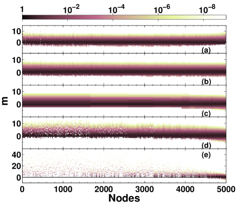
Figure 4: (Color online) The distribution of event sizes for biased random walks as a function of node number on $x$-axis obtained from simulations performed on a scale-free network for different values of bias parameters (a) $\alpha=-2.0$, (b) $\alpha=-1.0$, (c) $\alpha=0.0$, (d) $\alpha=1.0$ and (e) $\alpha=2.0$. The nodes are arranged in the order of increasing degree. The probability values $\mathcal{P}_{m}$ are color coded. This should be compared with analytical results in Fig. 5.

In comparison, for the case of $\alpha=1$ shown in Fig. 4(d) the events of size $8$ have higher probability of occurrence ($\mathcal{P}_{8}\sim 10^{-7})$ and events of even higher sizes are also possible. For $\alpha=2$, even higher size events, as large as 40, become highly probable for small degree nodes as seen in Fig. 4(e). Thus, in general, for larger $\alpha$, larger size events become probable when compared with the case of $\alpha=0$. Physically, this can be understood as follows. With $\alpha=0$, the random walkers perform unbiased random walk. However, for $\alpha=2$, the walkers preferentially choose to hop to nodes with larger degree (hubs). Since large degree nodes are mostly well connected among themselves, very few walkers reach small degree nodes. Hence the average flux through the small degree nodes becomes so small that even occasional visits by a few walkers lead to extremely large size events. These occasional visits lead to probability of order $10^{-6}$ even for events of size 40. Hence, in the case of biased random walks, extremely large fluctuations in event sizes can be observed in small degree nodes. This effect is also seen in the analytical results obtained using Eq. 15 shown in Fig. 5.

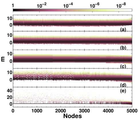
Figure 5: (Color online) The distribution of event sizes for biased random walks as a function of node number on $x$-axis obtained analytically using Eq. 15 for different values of bias parameter (a) $\alpha=-2.0$, (b) $\alpha=-1.0$, (c) $\alpha=0.0$, (d) $\alpha=1.0$ and (e) $\alpha=2.0$. The nodes are arranged in the order of increasing degree. The probability values $\mathcal{P}_{m}$ are color coded.

On the other hand, for cases $\alpha=-2,-1$ such large fluctuations are not visible in the event sizes in Fig. 4(a) and 4(b). For $\alpha=-1$ in Fig. 4(b), there is a small increase in the event sizes (when compared to $\alpha=0$) for the small degree nodes but it is not as large as in $\alpha=1$ case. Further, with $\alpha=-1$, it must also be noted that the probability profile remains similar for most of the nodes irrespective of the large differences in their degree. This is because $\phi$ is an approximate constant for most of the nodes since, in this case, the effect of the bias is balanced by the degree of these nodes. For $\alpha=-2$, the flux is strongly biased towards small degree nodes and again events of sizes $m=10$ can be seen in Fig. 4(a) though only on the higher degree nodes. The event sizes for hubs are not as large as observed in case of $\alpha=2$ for lower degree nodes. It can be explained as follows; when $\alpha=-2$, the flux preferentially flows through the small degree nodes which form the bulk in a scale-free network. Most small degree nodes do not have a direct link with other small degree nodes but are connected through a hub. Hence, despite the biased walk favoring the small degree nodes, sufficiently large flux flows through the hubs as well. Hence, abnormally large event size fluctuations are not seen in hubs for $\alpha=-1,-2$. All these features show a good agreement with the analytical result obtained in Eq. 15 and shown in Fig. 5.

V Discussion and summary

This work is an attempt to understand the extreme events occurring on the nodes due to flow on networks which typically is directed toward or away from the hubs. In this work, we study a biased random walk model in which the traffic preferentially moves either toward or away from the hubs and we analytically obtain the probabilities for the occurrence of extreme events. In this framework, extreme events are due to inherent fluctuations in the flux passing through any node and is defined as exceedences above a chosen threshold $q$. The threshold is chosen to be proportional to the natural variability of the node. Each node on the network is characterized by generalized strength $\phi$ which depends on its degree and that of its immediate neighbourhood. It is a measure of how much traffic is attracted to the particular node. The larger the generalized strength of a node is, larger its ability to attract walkers. In this paper, we have shown that the nodes with a smaller generalized strength, on an average, have a higher probability for the occurrence of extreme events when compared to nodes with higher generalized strength. Further, we have also shown that when the flux is biased toward the hubs, abnormally large fluctuations in event sizes become highly probable. This is one possible signature of the topologically biased flow in a scale-free network.

In general, it is possible to conceive of many ways by which bias can be imparted to independent random walkers on networks. These biasing strategies are motivated by real observations and the quest for efficient search strategies on networks. Various kind of biases based on the local environment, shortest paths, the entropy of random walk and various adaptive strategies are some examples of biased random walk on networks brw ; shw ; merw1 ; merw2 ; arw1 ; arw2 . It will be interesting to study the extreme event probabilities under such biasing strategies. However, we emphasise that if the stationary probability distribution equivalent to Eq. 5 exists for all the above strategies, then it would be possible to define extreme events and analyze them following the methods presented in this work.

In the context of scale-free network, it has been argued that hubs are important for better functioning of the network. Apart from being responsible for providing better connectivity, existence of hubs makes the scale-free network robust against the random node removal but fragile if the node removal is targeted node_del1 ; node_del2 . The results in this paper show that extreme events due to natural fluctuations are more probable on small degree nodes (when compared to the hubs). Hence special attention must be paid to designing the capacity of the small degree nodes so that extreme events can be smoothly handled without leading to disruption of the node. The results in this paper can be used to estimate the capacity a node should possess if it should handle extreme events of size, say, $m$. If we want the node to handle $4\sigma$ events smoothly, then the required capacity can be obtained by inverting Eq. 12. Thus, the numbers so obtained can be useful as an input for arriving at a capacity to be built for the nodes on a network.

- (1) S. Albeverio, V. Jentsch and Holger Kantz (Ed.) , Extreme events in nature and society, (Springer, 2005).
- (2) Stuart Coles An Introduction to Statistical Modeling of Extreme Values,(Springer, London, 2001)
- (3) http://blog.twitter.com/2010/02/measuring-tweets.html
- (4) http://www.comscore.com/Press_Events/Press_Releases/2010/1/Global_Search_Market_Grows_46_Percent_in_2009
- (5) U.S.-Canada Power System Outage Task force (April, 2004), see https://reports.energy.gov
- (6) D. De Martino, Luca Dall’Asta, Ginestra Bianconi and Matteo Marsili, Phys. Rev. E 79, 015101(R) (2009).
- (7) P. Echenique, J. Gomez-Gardenes and Y. Moreno, EPL 71, 325 (2005).
- (8) K. Kim, B. Kahng and D. Kim, EPL 86, 58002 (2009).
- (9) B. Tadic, G. J. Rodgers and S. Thurner, Int. J. Bifurcation Chaos Appl. Sci. Eng.17, 2363 (2007).
- (10) Douglas J. Ashton, T.C. Jarrett and N. F. Johnson, Phys. Rev. Lett. 94, 058701 (2005).
- (11) Liang Zhao, Ying-Cheng Lai, Kwangho Park and Nong Ye, Phys. Rev. E 71, 026125 (2005).
- (12) R. Germano and A.P.S. de Moura, Phys. Rev. E 74, 036117 (2006).
- (13) W. Wang, Zhi-Xi Wu, R. Jiang, G Chen and Y C Lai Chaos 19, 033106 (2009).
- (14) Vimal Kishore, M. S. Santhanam and R. E. Amritkar, Phys. Rev. Lett 106, 188701 (2011).
- (15) Agata Fronczak and Piotr Fronczak, Phys. Rev. E 80, 016107 (2009);
- (16) Wen-Xu Wang, B.H. Wang, C. Y. Yin, Y.B. Xie and T. Zhou, Phys. Rev. E 73, 026111 (2006).
- (17) S.-J. Yang, Phys. Rev. E 71, 016107 (2005).
- (18) J. D. Noh and H. Rieger, Phys. Rev. Lett. 92, 118701 (2004).
- (19) S. Meloni, J. Gomez-Gardenes, Vito Latora and Y. Moreno, Phys. Rev. Lett. 100, 208701 (2008).
- (20) J. L. Lopez and J. Sesma, Integral Transforms and Special Functions 8, 233 (1999).
- (21) V. Sood and P. Grassberger, Phys. Rev. Lett 99, 098701 (2007).
- (22) Shengyong Chen, Wei Huang, Carlo Cattani, and Giuseppe Altieri, Mathematical Problems in Engineering, 2012, 732698 (2012).
- (23) Z. Burda, J. Duda, J. M. Luck, and B. Waclaw, Phys. Rev. Lett. 102, 160602 (2009)
- (24) R. Sinatra, J. Gómez-Gardeñes, R. Lambiotte, V. Nicosia, and V. Latora, Phys. Rev. E 83, 030103(R) (2011).
- (25) B. Tadic, Eur. Phys. J. B 23,221 (2001).
- (26) A.N. Mian, R. Baldoni, R. Beraldi, Proceedings of the 29th IEEE International Conference on Distributed Computing Systems Workshops, Montreal, QC (IEEE, Piscataway, NJ,2009). pp. 153-157.
- (27) R. Cohen, K. Erez, ben-Avraham D. and S. Havlin, Phys. Rev. Lett 85, 4626 (2000).
- (28) R. Cohen, K. Erez, ben-Avraham D. and S. Havlin, Phys. Rev. Lett 86, 3682 (2001).