Also at ]Department of Physics, Technical University of Denmark, Lyngby 2800,Denmark Also at ]School of Physics, Tel Aviv University, Tel Aviv 69978, Israel And ]Israel Institute for Advanced Research IYAR, Rehovoth, Israel

Uncertainty Relation for Chaos

Abstract

A necessary condition for the emergence of chaos is given. It is well known that the emergence of chaos requires a positive exponent which entails diverging trajectories. Here we show that this is not enough. An additional necessary condition for the emergence of chaos in the region where the trajectory of the system goes through, is that the product of the maximal positive exponent times the duration in which the system configuration point stays in the unstable region should exceed unity. We give a theoretical analysis justifying this result and a few examples.

There are many systems for which local instability leads to chaotic behavior. It is often possible to characterize this local instability in terms of the divergence of orbits detected by computing Lyapunov exponents Gutzwiller , or by geometrical methods in cases where a geometric description becomes available, such as in the application of the Jacobi metric and the time dependence of the resulting Jacobi equation for geodesic deviation Gutzwiller ; PRE47 ; PRE48 ; PRL97 ; PRE96 for Hamiltonian systems, or the criteria based on the curvature of the dynamical manifold obtained from the recently developed geometric embedding method (GEM) Horwitz . These methods generally involve the computation of an exponential divergence as an indication of local instability. A given restricted region of exponential divergence, however, may not result in significant deviation of orbits, and therefore in chaotic behavior of the system. In this paper we give a quantitative bound which has the form of an uncertainty relation characterizing the effectiveness of the divergence in a locally unstable region. We find a relation between the time of passage of the orbit through an unstable region and the measure of instability, for example, a negative eigenvalue in the Jacobi equation, or the positive value of a Lyapunov exponent, which we denote in all these cases by $\lambda$, which results in stability. This relation is of the form of a product

$$\Delta t\cdot|\lambda|_{max}>1,$$ (1)

similar to that of an uncertainty relation between time and frequency in optics, or in quantum theory. The basis for this relation is that if there is an indication of exponential divergence, it is the time the system spends in the region of instability which determines whether the exponential divergence has reached a significant magnitude during this period. In general, the coefficient $\lambda$ is time dependent, but for a small region of instability, the relation equation (1) provides a useful measure. Moreover, this is a necessary condition of instability, and if it is not satisfied by the trajectories under study, one cannot expect chaotic behavior. Formula (1) is applied in several examples.

In a recent study Yahalom of the restricted three body problem, involving several configurations of an Earth, Sun, Jupiter type system, we successfully applied the geometric criterion of Horwitz based on a geometrical embedding of the Hamiltonian orbits derived from a conformal transformation of the original Hamiltonian of the form

$$H=\frac{p^{2}}{2m_{e}}+V(r,r_{j},r_{12})$$ (2)

where

$$V(r,r_{j},r_{12})=\frac{1}{2}m_{j}r_{j}^{2}\omega_{j}^{2}-\frac{4\pi^{2}m_{e}}{r}-\frac{4\pi^{2}m_{j}}{r_{j}}-\frac{4\pi^{2}m_{e}m_{j}}{r_{12}}.$$ (3)

This potential has an adiabatic time dependence due to the motion of the large planet (Jupiter) through the periodic dependence (frequency $\omega_{j}$ of its radial variable $r_{j}$; $r$ is the radial coordinate of the Earth from the Sun, and $r_{12}$ is the Earth- Jupiter distance). Although the GEM criterion was developed for time-independent potential systems, it was shown in Yahalom that the time dependence in this problem was negligible, provided the orbits did not pass too close to the boundaries of the physical region. Our prediction was that of stability with the exception of some small regions of instability near the foci (apsides) in highly eccentric orbits. These small regions of instability do not affect the overall stability of the system. In contrast, both Lyapunov methods and methods based on the time dependence of frequencies appearing in the application of the Jacobi metric, which predicted chaotic behavior for the system SafaaiSaadat , indicated instability over large regions of the orbits. One therefore must understand why exposure of the orbits to small regions of instability does not affect the outcome of the simulations, indicating completely stable behavior. These results were also obtained for the case of the Jupiter mass going to zero, for which the GEM method predicts the stability of the two-body Kepler problem correctly.

We have therefore investigated the application of the relation (1), and found that it was indeed fulfilled in these cases. We have furthermore applied the idea to other known potentially chaotic systems in dynamical regions (according to the choice of parameters) where the passage time multiplied by the maximum negative eigenvalue is small (but not zero) and found that these systems remained stable in this regime. Moreover, we found in these examples that as the parameters are changed to induce chaotic behavior, the degree of chaos was well correlated with the growth of the uncertainty product. This is consistent with the interpretation that the passage time for exponential deviations in the orbits induced by the time dependent eigenvalues of the Jacobi equation are critical in the development of chaos for such Hamiltonian systems. We have furthermore verified that a similar phenomenon occurs for the standard Lyapunov analysis in problems for which it is applicable. In the following we introduce a toy model for this phenomenon, and present results from simulations of motion based on a polynomial potential for the Hamiltonian system describing the Toda problem. We conclude with a discussion of the Kepler problem.

Assuming that we have two trajectories with a difference $\xi_{i}$, $i=1,2,3,...n$ in $n$ dimensions, we study a Jacobi equation with the simplifying assumption that we are close enough to the tangent space such that the covariant derivatives are well approximated by ordinary derivatives Gutzwiller , i.e., the geodesic deviation (Jacobi) equation is

$${\ddot{\xi}}_{i}=N_{ij}(t)\xi_{j}.$$ (4)

In the Lyapunov analysis:

$$N^{L}_{ij}=-\frac{1}{m_{i}}\frac{\partial^{2}V}{\partial x_{i}\partial x_{j}}$$ (5)

in which $x_{i}$ are the spatial degrees of freedom of the mechanical system, $V$ is the potential of the mechanical system and $m_{i}$ are the masses of the particles. In the GEM analysis Horwitz :

$$N^{G}_{ij}=-\frac{1}{m_{i}}\left(\frac{3}{2(E-V)}\frac{\partial V}{\partial x_{i}}\frac{\partial V}{\partial x_{j}}+\frac{\partial^{2}V}{\partial x_{i}\partial x_{j}}\right)$$ (6)

For a slowly varying matrix $N$ with a positive eigenvalue, $\xi$ may appear to be exponentially divergent on a small time interval. If we follow the orbit for some time, the maximum positive eigenvalue may go to zero, and the system will enter a stable regime. If the eigenvalue tends to zero sufficiently rapidly, the exponential divergence of the orbits, characterized by $\xi$, would not be adequate to lead to chaos. To see how this phenomenon can develop quantitatively, we compute the solution to the time dependent equation (4) in what follows.

Let us define ${\dot{\xi}}=\eta_{i}$; equation (4) can then be written

$${\dot{\zeta}}=M\zeta,$$ (7)

in which

$$\zeta=\left(\begin{array}[]{c}\xi\\ \eta\end{array}\right)$$ (8)

and

$$M=\left(\begin{array}[]{cc}0&I\\ N&0\end{array}\right)$$ (9)

where $I$ is a $n\times n$ unit matrix. Obviously the value of $\zeta$ cannot diverge faster than what is dictated by the maximal positive eigenvalue of $M$ over a certain duration. Let us now look at a specific example. For a $2\times 2$ (2D) $N$ we have a $4\times 4$ $M$. The eigenvalues $\lambda$ of $N$ are then determined by:

$$\lambda^{2}-\lambda{\rm Tr}N+\det{N}=0$$ (10)

The eigenvalues $\mu$ of $M$ are determined by

$$\mu^{4}-\mu^{2}{\rm Tr}N+\det{N}=0.$$ (11)

so that $\mu^{2}=\lambda$. Then, local stability is determined by

$$\lambda>0:\mu\ {\rm real,unstable}$$

$$\lambda<0,\mu\ {\rm imaginary,stable}$$ (12)

It might be convenient to take

$$N=aI+b\sigma_{1}+c\sigma_{3}\qquad(\sigma_{i}{\rm\ is\ a\ Pauli\ matrix})$$ (13)

as a real symmetric example. Then,

$$N=\left(\begin{array}[]{cc}a+c&b\\ b&a-c\end{array}\right),$$ (14)

and the eigenvalues become:

$$\lambda_{\pm}=a\pm\sqrt{b^{2}+c^{2}}.$$ (15)

Now let us assume that:

$$b=\rho\cos{\theta},\qquad c=\rho\sin{\theta},$$ (16)

where $\rho>0$ and $\theta$ are some arbitrary parameters. In this form the eigenvalues will take the form:

$$\lambda_{\pm}=a\pm\rho.$$ (17)

Notice that the value of $\theta$ does not effect the eigenvalues and hence we will take it as $\theta=0$. Moreover by proper temporal scaling we can always take $\rho=1$. For $a=-|a|<0$, the eigenvalue $\lambda_{-}$ is negative and hence always stable; we thus need to analyze only the behavior of $\lambda_{+}$. The following form for $a$ is assumed:

$$a=-\frac{t}{\Delta t}$$ (18)

for which $\Delta t>0$ is some given time interval. The eigenvalues are then:

$$\lambda_{\pm}=-\frac{t}{\Delta t}\pm 1.$$ (19)

In particular, $\lambda_{+}=1-\frac{t}{\Delta t}$ is positive for $t<\Delta t$ (and hence unstable) but negative for $t>\Delta t$ and hence stable. This model is therefore appropriate in order to study the effect of the duration of the trajectory in the unstable region on the systems overall stability. The maximal instability exponent is $\lambda_{+max}=1$ at $t=0$. Thus equation (1) takes the simple form:

$$\Delta t>1$$ (20)

as a necessary (but not sufficient condition) of instability. To appreciate the significance of the above result let us look at two trajectories displaced at $t=0$ by an amount $\vec{\xi}=(1,0)$ but with the same velocity $\vec{\eta}=(0,0)$. In the case $\Delta t=5$ depicted in figure 1, it is clearly seen that the exponential growth (black line) is not achieved by either component of $\vec{\xi}$. We see a growth by an order of magnitude in the size of the displacement $\xi_{1}$, the displacement $\xi_{2}$ achieves the same magnitude as $\xi_{1}$ although null at $t=0$ due to the coupling with $\xi_{1}$. The entire growth happens at an interval slightly longer than $\Delta t=5$ including a slight overshot. Entering the stable region the displacements oscillate with a constant amplitude. Let us now consider the case in which equation (20) is not satisfied, for example let $\Delta t=0.1$; this case is depicted in figure 2. One can hardly notice the exponential growth in figure 2; as to $\xi_{1}$ and $\xi_{2}$ the fact that the ”unstable” region is so minute does not allow them to grow at all and they oscillate at an amplitude smaller than the original displacement. Having demonstrated the chaotic uncertainty principle with a toy model we now move on to more realistic examples.

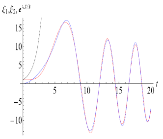
Figure 1: The case $\Delta t=5$, the figure depicts $\xi_{1}(t)$ $(\xi_{1}(0)=1)$ by a red line, $\xi_{2}(t)$ $(\xi_{2}(0)=0)$ by a blue line while the black line describes an exponential growth according to the maximal exponent $\lambda_{+max}=1$. (color online)

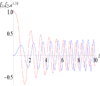
Figure 2: The case $\Delta t=0.1$, the figure depicts $\xi_{1}(t)$ $(\xi_{1}(0)=1)$ by a red line, $\xi_{2}(t)$ $(\xi_{2}(0)=0)$ by a blue line while the black line describes an exponential growth according to the maximal exponent $\lambda_{+max}=1$. (color online)

A generalization of the Toda potential is described by BenZion ; in this model the potential of the two-dimensional system is given by:

$$V(x,y)=\frac{1}{2}(x^{2}+y^{2})+x^{2}y-\frac{1}{3}y^{3}+\frac{3}{2}x^{4}+\frac{1}{2}y^{4}$$ (21)

Considering a unit mass, it was shown previously in BenZion that for energy $E$ somewhat larger than $0.2$ the system becomes chaotic. Calculating the value of $\lambda\Delta t$ in which $\Delta t$ is the duration spent in unstable regions, one arrives at figure 3. It is clearly

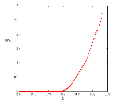
Figure 3: The product of $\lambda$ with the time spent in unstable regions $\Delta t$ vs. energy. As the product becomes appreciable, the increase of chaotic behavior is seen clearly on Poincaré plots.(color online)

seen that the product of $\lambda$ with the time spent in unstable regions only reaches considerable size when the system becomes chaotic, that is when $E>0.215$. The Poincaré plots for $0.2<E<0.215$ does not show chaotic behavior since the product of $\lambda$ with the time spent in the unstable region is not considerable. This is shown in figure 4. The Lyapunov exponent just below the chaotic threshold of $E=0.2$ (not shown here) predicts chaotic behavior which is not manifested; this is another indication of the effectiveness of the GEM method.

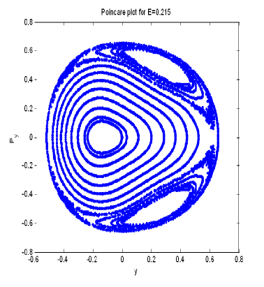
Figure 4: The Poincaré plot for $E=0.215$. For this value $\lambda\Delta t=1.044$ and a very mild chaotic behavior is seen as predicted by the chaotic uncertainty relation. (color online)

It is well known that the Kepler orbit which is clearly integrable and not chaotic, is predicted to be chaotic according to the Lyapunov stability criterion. At least one Lyapunov exponent is positive throughout the orbit indicating all over instability. In contrast, the geometric method developed by Horwitz et al. Horwitz generates the correct sign of the corresponding exponent. The same is true for the restricted three-body problem in which a ”Jupiter” is constrained to move on a large circular trajectory Yahalom . This system is described by equations (2) and (3). The above statement is true for low eccentricity orbits, however for high eccentricity orbits such as the one depicted in figure 5 even the GEM method suffers from local unstable exponents near the perihelion. Nevertheless, a calculation of the product of the exponent times the duration it takes the orbit to go through the unstable region indicates that the necessary condition (1) of instability is not met. For example the orbit of figure 5 exhibits

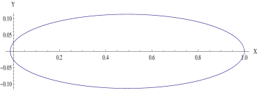
Figure 5: A high eccentricity orbit. (color online)

a positive geometric exponent near the perihelion (being stable everywhere else) of the form described in figure 6.

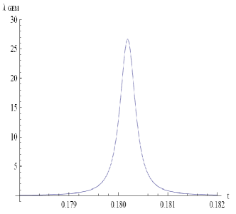
Figure 6: The geometric eigenvalue of the Keplerian orbit near perihelion. (color online)

For this unstable region we have $\lambda_{max}\Delta t\simeq 0.6$, which is below what is required for chaotic instability. The Lyapunov criterion, however, implies instability over the entire orbit.

Our analysis of the Kepler problem and the restricted three body problem using the GEM method has led us to investigate the meaning of localized instabilities. This in turn has led us to formulate the chaotic uncertainty principle of equation (1). The content of the idea was investigated through a toy model demonstrating that unless the condition is met one cannot expect small deviations to grow by more than an order of magnitude. The value of this idea was further underlined in the generalized Toda potential. Finally it proved most valuable in understanding the ineffectiveness of the very local indications of instability arising in the Kepler and three-body orbits that appear in the GEM analysis. We foresee the usefulness of the idea for studying chaotic systems in general.

References

- (1) 9
- (2) M.C. Gutzwiller, Chaos in Classical and Quantum Mechanics, Springer-Verlag, New York (1990). See also W.D. Curtis and F.R. Miller, Differentiable Manifolds and Theoretical Physics, Academic Press, New York (1985), J. Moser and E.J. Zehnder, Notes on Dynamical Systems, Amer. Math. Soc., Providence (2005), and L.P. Eisenhardt, A Treatise on the Differential Geometry of Curves and Surfaces, Ginn, Boston (1909) [Dover, N.Y. (2004)].
- (3) M. Pettini, Phys. Rev. E 47, 828 (1993).
- (4) L. Casetti and M. Pettini, Phys. Rev. E 48, 4320 (1993).
- (5) L. Caiani, L.Castti, and M. Pettini, Phys Rev. Lett. , 4631 (1997).
- (6) L. Casetti. C. Clementi and M. Pettini Phys. Rev. E 54, 5969 (1996).
- (7) L.Horwitz, Y. Ben Zion, M. Lewkowicz, M. Schiffer and J. Levitan, Phys. Rev. Lett, 98, 234301 (2007).
- (8) Y. Ben Zion and L. Horwitz, Phys. Rev. E 78, 036209 (2008).
- (9) A. Yahalom, J. Levitan, M. Lewkowicz and L. Horwitz ”Lyapunov vs. Geometrical Stability Analysis of the Kepler and the Restricted Three Body Problem” Physics Letters A, Volume 375, Issue 21, 23 May 2011, Pages 2111-2117. doi:10.1016/j.physleta.2011.04.016
- (10) H. Safaai, M. Hasan and G. Saadat, Understanding Complex Systems (Springer Berlin, 2006).