Classical dynamics of strings and branes,
with application to vortons
Brandon Carter
LUTH (CNRS), Observatoire Paris - Meudon
Invited contribution. to Proc. JGRG20,
ed. T. Hiramatsu, M. Sasaki, M. Shibata, T, Shiromizu,
Yukawa Institute, Kyoto, September, 2010.
Abstract. These notes offer an introductory overview of the essentials of classical brane dynamics in a space-time background of arbitrary dimension, using a systematic geometric treatment emphasising the role of the second fundamental tensor and its trace, the curvature vector . This approach is applied to the problem of stability of vorton equilibrium states of cosmic string loops in an ordinary 4-dimensional background.
1 Worldsheet Curvature Analysis
1.1 The first fundamental tensor
Earlier treatments of the classical dynamics of strings and higher p-branes were inclined to rely too much on gauge dependent auxiliary structures such as internal coordinates on the d=p+1 dimensional worldsheet, which can be useful for various computational purposes but tend to obscure what is essential. The present notes offer an introductory overview of a more geometrically elegant approach [2] that is particularly useful for work in a background spacetime whose dimension n is 5 or more [3, 4, 5], but that I originally developed for the purpose of studying cosmic string loops and particularly the question of the stability of their vorton equilibrium states [6] in a background of dimension n=4. Following the strategy originally advocated by Stachel[7], the guiding principle of this approach [2] is to work as far as possible with a single kind of tensor index, which must of course be the one that is most fundamental, namely that of the n-dimensional coordinates, on the background spacetime with metric
The idea is to avoid unnecessary use of the internal coordinate indices, which are lowered and raised by contraction with the induced metric (using the notation ) on the worldsheet, and with its contravariant inverse This is achieved by working instead with the (first) fundamental tensor as given by projection back onto the background according to the prescription
| (1) |
(in the manner that is applicable to the contravariant version of any worldsheet tensor) so that will be the tangential projector. The complementary orthogonal projector is As well as having the properties and these projection tensors will evidently be related by
1.2 The second fundamental tensor
In so far as we are concerned with tensor fields such as the frame vectors whose support is confined to the d-dimensional world sheet, the effect of Riemannian covariant differentation along an arbitrary directions on the background spacetime will not be well defined, only the corresponding tangentially projected differentiation operation
| (2) |
being meaningful for them, as for instance in the case of a scalar field for which the tangentially projected gradient is given in terms of internal coordinate differentiation simply by The action of this operator on the first fundamental tensor itself gives the entity
| (3) |
that we refer to [2] as the second fundamental tensor.
As this second fundamental tensor, will play an important role in the work that follows, it is worth lingering [2] over its essential properties. The expression (3) could of course be meaningfully applied not only to the fundamental projection tensor of a d-surface, but also to any (smooth) field of rank-d projection operators as specified by a field of arbitrarily orientated d-surface elements. What distinguishes the integrable case – in which the elements mesh together to form a well defined d-surface through the point under consideration – is the Weingarten identity, whereby that the tensor defined by (3) will have the symmetry property
| (4) |
an integrability condition that is derivable [2] as a version of the well known Frobenius theorem.
As well as being symmetric, the tensor is obviously tangential on the first two indices and also orthogonal on the last: It fully determines the tangential derivatives of the first fundamental tensor by the formula
| (5) |
(using round brackets to denote symmetrisation) and it is characterisable by the condition that the orthogonal projection of the acceleration of any tangential unit vector field (with ) will be given by
1.3 Extrinsic curvature vector and Conformation tensor
It is very practical for a great many purposes to introduce the extrinsic curvature vector defined [2] as the trace of the second fundamental tensor,
| (6) |
which is automatically orthogonal to the worldsheet, It is useful for many specific purposes to work this out in terms of the intrinsic metric and its determinant . For the tangentially projected gradient of a scalar field on the worldsheet, it suffices to use the simple expression However for a tensorial field (unless one is using Minkowski coordinates in a flat spacetime) the gradient will also have contributions involving the background Riemann Christoffel connection The curvature vector is thus obtained in explicit detail as
| (7) |
This expression is useful for specific computational purposes, but much of the literature on cosmic string dynamics has been made unnecessarily heavy by a tradition of working all the time with long strings of non tensorial terms such as those on the right of (7) rather than exploiting more succinct tensorial expressions, such as
As an alternative to the universally applicable tensorial approach advocated here, there is of course another more commonly used method of achieving succinctness in particular circumstances, which is to sacrifice gauge covariance by using specialised kinds of coordinate system. In particular, for the case of a string, i.e. for a 2-dimensional worldsheet, it is standard practise to use conformal coordinates and so that the corresponding tangent vectors and satisfy the restrictions which implies so that (7) simply gives
The physical specification of the extrinsic curvature vector (6) for a timelike d-surface in a dynamic theory provides what can be taken as the equations of extrinsic motion of the d-surface [2], the simplest possibility being the “harmonic” condition that is obtained (as shown below) from a surface measure variational principle such as that of the Dirac membrane model [8], or of the Goto-Nambu string model [9] whose dynamic equations in a flat background are therefore expressible with respect to a standard conformal gauge in the familiar form
There is a certain analogy between the Einstein vacuum equations, which impose the vanishing of the trace of the background spacetime curvature and the Dirac-Gotu-Nambu equations, which impose the vanishing of the trace of the second fundamental tensor Moreover, just as it is useful to separate out the Weyl tensor [10], i.e. the trace free part of the Ricci background curvature which is the only part that remains when the Einstein vacuum equations are satisfied, so also analogously, it is useful to separate out the the trace free part of the second fundamental tensor, namely the extrinsic conformation tensor [2], which is the only part that remains when equations of motion of the Dirac - Goto - Nambu type are satisfied.
Explicitly, the trace free extrinsic conformation tensor of a d-dimensional imbedding is defined [2] in terms of its first and second fundamental tensors as
| (8) |
Like the Weyl tensor of the background metric (whose definition is given implicitly by (13) below) this conformation tensor has the noteworthy property of being invariant with respect to conformal modifications of the background metric:
| (9) |
This is useful [11] for work like that of Vilenkin [12] in a Robertson-Walker cosmological background, which can be obtained from a flat spacetime by a conformal transformation for which is a time dependent Hubble expansion factor.
1.4 Codazzi, Gauss, and Schouten identities
As the higher order analogue of (3) we can go on to introduce the third fundamental tensor[2] as
| (10) |
which by construction is obviously symmetric between the second and third indices and tangential on all the first three indices. In a spacetime background that is flat (or of constant curvature as is the case for the DeSitter universe model) this third fundamental tensor is fully symmetric over all the first three indices by what is interpretable as the generalised Codazzi identity.
In a background with arbitrary Riemann curvature the generalised Codazzi identity is expressible [2] as
| (11) |
A script symbol is used here in order to distinguish the ( n- dimensional) background Riemann curvature tensor from the intrinsic curvature tensor of the ( d- dimensional) worldsheet to which the ordinary symbol has already allocated. For many of the applications that will follow it will be sufficient just to treat the background spacetime as flat, i.e. to take
For , the background curvature tensor will be decomposible (if present) in terms of the background Ricci tensor and its scalar trace,
| (12) |
and of its trace free conformally invariant Weyl part – which can be non zero only for 4 – in the well known [10] form
| (13) |
In terms of the tangential projection of this background curvature, the corresponding internal curvature tensor takes the form
| (14) |
which is the translation into the present scheme of what is well known in other schemes as the generalised Gauss identity.
The less well known analogue (attributable [10] to Schouten) for the (trace free conformally invariant) outer curvature is expressible [2] in terms of the relevant projection of the background Weyl tensor as
| (15) |
In a background that is flat or conformally flat (for which it is necessary, and for sufficient, that the Weyl tensor should vanish) the vanishing of the extrinsic conformation tensor will therefore be sufficient (independently of the behaviour of the extrinsic curvature vector ) for vanishing of the outer curvature tensor which is the condition for it to be possible to construct fields of vectors orthogonal to the surface and such as to satisfy the generalised Fermi-Walker propagation condition to the effect that should vanish.
2 Laws of motion for a regular brane complex
2.1 Definition of brane complex
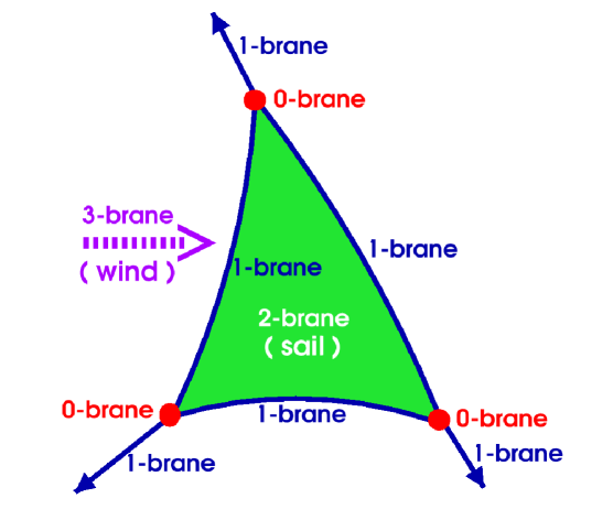
The term p-brane has come [13, 14] to mean a dynamic system localised on a timelike support surface of dimension d= p+1 , in a spacetime background of dimension n p . Thus a zero - brane means a “point particle”, and a 1-brane means a “string”, while a 2-brane means what is commonly called a “membrane”. At the upper extreme an ( n-1)-brane is what is commonly referred to as a “medium” (as exemplified by a simple fluid). The codimension-1 (hypersurface supported) case of an ( n-2)-brane (as exemplified by a cosmological domain wall) is what may be referred to as a “hypermembrane”, while the codimension-2 case of an ( n-3)-brane is what may analogously be referred to as a “hyperstring”.
A set of branes forms a “brane complex” if the support surface of each ( d-1)-brane member is a smoothly imbedded d-dimensional timelike submanifold of which the boundary, if any, is a disjoint union of support surfaces of lower dimensional members of the set. For the complex to qualify as regular [2] it is required that a p-brane member can act directly only on an ( p-1)-brane member on its boundary or on a -brane member on whose boundary it is itself located, though it may be passively influenced by higher dimensional background fields.
Direct mutual interaction between branes with dimension differing by 2 or more would usually lead to divergences, symptomising the breakdown of a strict – meaning thin limit – brane description. To cure that properly, a more elaborate treatment – allowing for finite thickness – would be needed, but it may suffice to use a thin limit approximation [16] whereby the divergence is absorbed [17, 18] in a renormalisation.
In the case of a brane complex, the total action will be given as a sum of contributions from the various (d-1)-branes of the complex, of which each has its own Lagrangian d-surface density scalar say. Each supporting d-surface will be specified by a mapping giving the local background coordinates ( = 0, …. , n-1) as functions of local internal coordinates ( = 0, … , d-1). The corresponding d-dimensional surface metric tensor induced as the pull back of the n-dimensional background spacetime metric determines the surface measure, in terms of which the total action will be expressible as
| (16) |
2.2 Conserved current and the stress-energy tensor
As well as on its own internal (d-1)-brane surface fields and their derivatives, and those of any attached d-brane, each contribution will also depend (passively) on the spacetime metric and perhaps other background fields, of which the most common example is a Maxwellian gauge potential for which the corresponding field is invariant under gauge changes and is automatically closed, Subject to the internal dynamic equations of motion given by the variational principle stipulating preservation of the action by variations of the independent field variables, the effect of arbitrary infinitesimal “Lagrangian” variations of the background fields will be to induce a corresponding variation
| (17) |
from which, for each -brane, one can read out the electromagnetic surface current vector and also (since ) the surface stress momentum energy tensor
| (18) |
For any d-dimensional support surface Green’s theorem gives
| (19) |
taking the integral on the right over the boundary (d-1)-surface of of where is the (uniquely defined) outward directed unit tangent vector on the d-surface at its ( d-1)-dimensional boundary.
The Maxwell gauge invariance condition (independence of ) is thus seen to be equivalent to the electric current conservation condition
| (20) |
which means that the source of charge injection into any particular (p-1)-brane is the sum of the currents flowing in from the p-branes to which it is attached.
2.3 Force and the stress balance equation
The condition of being “Lagrangian” means that is comoving as needed to be meaningful for fields with support confined to a particular brane. However for background fields one can also define an “Eulerian” variation, , with respect to some appropriately fixed reference system, in which the infinitesimal displacement of the brane complex is specified by a vector field The difference will be given by where the is the Lie differentiation operator, which will be given for the relevant background fields by the familiar formulae and
In a fixed Eulerian background, the background fields will have Lagrangian variations given just by their Lie derivatives with respect to the displacement . Subject to the internal field equations, the action variation due to the displacement of the branes will therefor just be The postulate that this vanishes for any entails the further d-surface tangentiality restriction and (by the Green theorem) the dynamic equations
| (21) |
in which total force density,
| (22) |
includes the Faraday-Lorenz contribution from the background, while on each ( p-1)-brane, the contact force exerted by attached p-branes is
| (23) |
in which it is to be recalled that, on the ( p+1)-dimensional support surface of each attached -brane, is the unit vector that is directed normally towards the bounding ( p-1)-brane.
The tangential force balance equations will hold as identities when the internal field equations are satisfied (because a surface tangential displacement has no effect). The non-redundent information governing the extrinsic motion of a -brane will be given just by the orthogonal part. Integrating by parts, as the surface gradient of the rank- orthogonal projector will be given in terms of the second fundamental tensor of the -surface by
| (24) |
the extrinsic equations of motion are finally obtained in the form
| (25) |
It is to be remarked that this is valid not just for a conservative force such as the electromagnetic example considered above, but also for dissipative forces such as frictional drag[11] by a relatively moving background medium.
The most familiar application is to the case of a point particle of mass m with unit velocity vector and orthogonally directed acceleration vector for which one has so that and
3 Canonical Liouville and symplectic currents
3.1 Canonical formalism for Branes
For the study of small perturbations, and particularly for the systematic derivation of conservation laws associated with symmetries, it is useful to employ a treatment of the canonical kind that was originally developped in the context of field theory (as a step towards quantisation) by Witten, Zuckerman, and others [19, 20, 21, 22, 23, 24, 25]. This section describes the generalisation of this procedure to brane mechanics in the manner initiated by Cartas-Fuentevilla [26, 27] and developed in collaboration with Dani Steer [28]. After a general presentation, including a review of the relationships between the various (Lagrangian, Eulerian and other) relevant kinds of variation, the procedure is illustrated by application to a particular category that includes the case of branes of purely elastic type.
Consider a generic conservative p-brane model whose mechanical evolution is governed by an action integral of the form
| (26) |
over a supporting worldsheet with internal co-ordinates and induced metric in a background with coordinates and (flat or curved) space-time metric The relevant Lagrangian scalar density is given as a function of a set of field components – including background coords – and of their surface deriatives, The relevant field variables can be of internal or external kind, the most obvious example of the latter kind being the background coordinates themselves.
The generic action variation,
| (27) |
specifies partial derivative components and and corresponding generalised momentum components The variation principle characterises dynamically admissible “on shell” configurations by the vanishing of the Eulerian derivative
| (28) |
In terms of this Eulerian derivative, the generic Lagrangian variation will have the form
| (29) |
There will be a corresponding pseudo-Hamiltonian scalar density
| (30) |
for which
| (31) |
(The covariance of such a pseudo-Hamiltonian distingushes it from the ordinary kind of Hamiltonian, which depends on the introduction of some preferred time foliation.)
For an on-shell configuration, i.e. when the dynamical equations
| (32) |
are satisfied, the Lagrangian variation will reduce to a pure surface divergence,
| (33) |
and the correponding on-shell pseudo-Hamiltonian variation will take the form
| (34) |
3.2 Symplectic structure
The generic first order variation of the Lagrangian will be given by
| (35) |
in terms of the generalised Liouville 1-form (on the configuration space cotangent bundle) defined by
| (36) |
Now consider a pair of successive independent variations which will give a second order variation of the form
| (37) |
Thus using the commutation relation one gets
| (38) |
where the symplectic 2-form (on the configuration space cotangent bundle) is defined by
| (39) |
For an on-shell perturbation we thus obtain
| (40) |
while for a pair of on-shell perturbations we obtain
| (41) |
The foregoing surface current conservation law is expressible in shorthand as
| (42) |
in which the closed (since manifestly exact) symplectic 2-form (39) is specified in concise wedge product notation as
| (43) |
Some authors prefer to use an even more concise notation system in which it is not just the relevant distinguishing (in our case acute and grave accent) indices that are omitted but even the wedge symbol that indicates the antisymmetrised product relation. However such an extreme level of abbreviation is dangerous [26] in contexts in which symmetric products are also involved.
3.3 Translation into strictly tensorial form
To avoid the gauge dependence involved in the use of auxiliary structures such as local frames and internal surface coordinates, by working [29] just with quantities that are strictly tensorial with respect to the background space, one needs to replace the surface current densities whose components and depend on the choice of the internal coordinates by vectorial quantities with strictly tensorial background coordinate components given by
| (44) |
and with strictly scalar divergences given by
| (45) |
In terms of the surface projected covariant differentiation operator defined in terms of the fundamental tensor by one thus obtains a Liouville current conservation law of the form
| (46) |
for any symmetry generating perturbation, i.e. for any infinitesimal variation such that Similarly a symplectic current conservation law of the form
| (47) |
will hold for any pair of perturbations that are on-shell, i.e. such that
3.4 Application to hyperelastic case
In typical applications, the relevant set of configuration components will include a set of brane field components as well as the background coords , so that in terms of displacement vector the Liouville current will take the form
| (48) |
in which the latter version replaces the original momentum components by the corresponding background tensorial momentum variables, which are given by and
The hyperelastic category [30] (generalising the case of an ordinary elastic solid which includes the special case of an ordinary barotropic perfect fluid) consists of brane models in which – with respect to a suitably comoving internal reference system – there are no independent surface fields at all – meaning that the and the are absent – and in which the only relevant background field is the metric that is specified as a function of the external coordinates . In any such case, the generic variation of the Lagrangian is determined just by the surface stress momentum energy density tensor according to the standard prescription
| (49) |
whereby is specified in terms of partial derivation of the action density with respect to the metric.
In a fixed background (i.e. in the absence of any Eulerian variation of the metric) the Lagrangian variation of the metric will be given by Comparing this to canonical prescription with shows that the relevant partial derivatives will be given by the (non-tensorial) formulae It can thus be seen that in the hyperelastic case, the canonical momentum tensor and the Liouville current will be given just in terms of surface stress tensor by the very simple formulae
| (50) |
In order to proceed, we must consider the second order metric variation, whereby (following Friedman and Schutz [31]) the hyper Cauchy tensor (generalised elasticity tensor) is specified [32] in terms of Lagrangian variations by a partial derivative relation of the form
| (51) |
The symplectic current is thereby obtained in the form
| (52) |
where
| (53) |
4 Brane perturbation by gravitational radiation
4.1 Generic case
A background metric perturbation will provide an extra Lagrangian and stress contributions and whence a corresponding force increment The effect of this is expressible as the inclusion of an extra term on the right of the original force balance equation, as expressed in terms of the unperturbed values of the metric stress tensor and force density so as to obtain a perturbed force balance of the form
| (54) |
in which the effective gravitational perturbation contribution is given by
| (55) |
a formula that was not so well known until relatively recently [32].
4.2 The case of a simple Dirac-Nambu-Goto type brane
The simplest dimensionally unrestricted application, is to a p-brane of the Dirac-Nambu-Goto type, for which the relevant master function is simply constant, so given in terms of a corresponding Kibble mass by (In the context of superstring theory is typically of the order of magnitude of the Planck mass , whereas in the context of cosmic string theory the Kibble mass is expected to comparable with the relevant Higgs mass, ) In this special case, the surface stress momentum energy tensor is of course simply proportional to the fundamental tensor:
| (56) |
so its trace will be given by ( p+1) where is interpretable as the surface tension. The corresponding the hyper-Cauchy tensor is found[32] to be
| (57) |
The dynamical equation of motion (54) will therefor reduce to the form
| (58) |
in which (as well as the possibility of drag) the right hand side will include an effective gravitational contribution expressible[32] in the form with
| (59) |
| (60) |
It was observed by Battye[33, 34] that the early work on gravitational perturbations of strings cited by Vilenkin and Shellard in their 1994 treatise [35] was seriously flawed by the use for estimating of a formula (7.7.3) without the orthogonal projection operator in the expression (59) for and entirely lacking the contribution which might be relatively negligible for high frequency radiation[33] of external origin, but not in the case of self-interaction for which the two contributions will be comparable. The self interaction contributions from (59) and (60) will be separately divergent, but in the “hyperstring” case these divergences will actually cancel each other. Thus (contrary to what was claimed in (7.7.7) [35]) the total self-interaction will remain finite[34, 17, 18] whenever the codimension is 2, as for an ordinary string in 4 dimensions (or for a “brane-world” in 6 dimensions).
4.3 Regularisation of self-interaction
To treat such self-interaction one must face the problem that the regularity condition (see Figure 1) is violated whenever a brane of dimension acts on a background of dimension . To cure this, a physically realistic regularisation involves replacing the infinitely thin worldsheet by a support of finite thickness. The divergent self-interaction fields such as and are then replaced by regularised averages and with dominant contribution proportional to the relevant source [17, 18]. This means and which for a Nambu-Goto hyperstring, gives with a proportionality coefficient that diverges as the thickness tends to zero. On such world sheet confined fields, the ordinary gradient operator must be replaced by the corresponding regularised operator so that for example the field will have the regularised average as needed for the electromagnetic self-interaction force density The required result, giving zero gravitational contribution, for Nambu-Goto hyperstrings (including [34] the ordinary string case p=1 with n=4) has been shown [16] to be provided generally by the conveniently simple and easily memorable formula
5 Vorton equilibrium states of elastic string loops
5.1 The category of simple elastic string models
For any string model the fundamental tensor of the 2 dimensional worldsheet will be expressible in terms of any orthonormal diad of space like and timelike vectors as There will generically be a prefered diad with respect to which the symmetric surface stress energy tensor will be expressible as
| (61) |
where is the string tension, and is the surface energy density, which, in the elastic case, is determined as a function of by an equation of state.
In addition to the extrinsic (transversely polarised)“wiggle” perturbations which, as in any string model, travel with a characteristic velocity such a model has perturbation modes of only one other kind: these are sound type (longitudinal compression) “woggle” modes, which propagate relative to the locally preferred frame with speed given by the formula . A particularly important special case is that of models of the integrable transonic type [36] for which the “wiggle” and “woggle” speeds coincide, which occurs when the equation of state is specified simply by the specification of a fixed value for the product . The kind of model appropriate for representing such familiar technical applications as bow strings, or the strings of musical instruments, will generally be of subsonic type, meaning that the wiggle speed is less than the sonic speed , while on the other hand it has been shown by Peter [37] that models of supersonic type will commonly be needed for the representation of cosmic strings of the conducting vacuum vortex type envisaged by Witten [38].
A model of any such elastic type is specifiable in variational form by a string Lagrangian depending only on the magnitude of the gradient of some stream function (which in the Witten case represents the phase of a complex scalar field). This means that the string model is characterised by a single variable equation of state giving as a function of the scalar It is useful [15, 39] to introduce the corresponding adjoint formulation in terms of the quantity with When , one finds that the tension and energy density will be given by while when they will be given by In all cases the phase gradient is proportional to a surface current, that has the property of being conserved, whenever there is no external force, so that the equation of motion of the worldsheet reduces to the simple form with
When he originally introduced the concept of conducting cosmic strings [38] Witten suggested that a simple linear action formula, involving just a single extra parameter (namely a lengthscale ) might be used as a good approximation, least in the weak current limit for which is sufficiently small. However it subsequently became clear that such a linear formula is inadequate even in the weak current limit, since it implies that wiggle propagation would always be subsonic , whereas detailed examination of the relevant kind of vacuum vortex by Peter [37] revealed that the wiggle propagation in such a case would typically be supersonic As a more satisfactory replacement for Witten’s direct linearity ansatz, it has been found [40, 41] that at the cost of introducing one more mass scale a reasonably good representation is obtainable by using an ansatz of logarithmic form
5.2 Stationary string states in flat background
We shall conclude this overview by considering what can be said about stationary equilibrium states, as characterised, in a flat background a world sheet that is tangent to a timelike unit static Killing vector satisfying . In such a worldsheet there will also be an orthogonal (and therefor spacelike) unit tangent vector satisfying the invariance condition For such a worldsheet, the first fundamental tensor will be given by while in terms of the curvature vector, the second fundamental tensor will be given by
Within the worldsheet, the preferred timelike eigenvector of the stress energy tensor, as characterised by the relation will be expressible in the form
| (62) |
which defines the relative flow velocity Under these conditions, the free dynamical equation (5.1) can be seen to reduce to the simple form
For an infinitely long string this equation can of course be solved in a trivial manner by choosing a configuration that is straight, which means in which case the value of is unrestricted. However for a finite closed loop the curvature cannot vanish everywhere, and where is non-zero the only way of satisfying the extrinsic equilibrium condition(5.2) is for the relative flow velocity to bethe same as the relevant wiggle propagation speed: while to satisfy the intrinsic (current conservation) equilibrium condition it is trivially sufficient (and generically necesssary) for the value of this speed to be uniform. Provided this centrifugal equilibrium condition is satisfied, there is no retriction on the curvature, which need not be uniform: thus the equilibrium configuration of the string loop need not be circular, but may have an arbitrary shape.
5.3 Stability criterion for circular vorton states
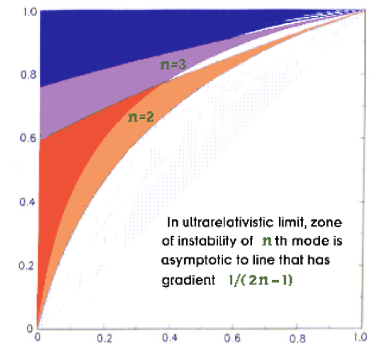
It is easy to see that the stability of a uniform circular equilibrium state of an elastic string loop in a flat background will depend just on the extrinsic (wiggle type) and longitudinal (sound type) perturbation speeds, and . Moreover it is fairly easy to show [6] that such a state will always be stable in the subsonic case, , which is what is most likely to be relevant in a terrestrial engineering context.Even in the supersonic case, it has been shown [6] that monopole and dipole perturbation modes are always stable. However instability may occur for higher modes, for which, in a state with radius the eigenfrequency is given by the solution of an equation of the cubic form for the quantity where is the relative velocity of orthogonaly polarised forward propagating wiggles, and the coefficients of the cubic are given by using the notation
The stability criterion, for all the roots to be real, is the positivity of a discriminant Figure 2 shows the zones of negativity (instability) for the lowest relevant mode numbers, by Martin [42]. In the ultrarelativistic limit , that is relevant for weak currents in conducting cosmic strings, one gets and
| (63) |
which is strictly positive (implying stability) almost always, the unstable exceptions being on the lines converging in the plot to the limit point , with gradient given in terms of the corresponding node number by
The upshot is that although some circular vorton states are unstable, there are plenty more – the ones that would presumably be selected under natural conditions – that are stable, at least with respect to macroscopic string perturbations. It is however to be remarked that – since it deals only with the thin string limit – the kind of analysis described here can not resolve the (sensitively model dependent) issue of stability with respect to quantum effects or other processes involving the microscopic internal structure of the vacuum vortex or whatever else may constitute the string.
Références
- [1]