Constraining the interior of extrasolar giant planets with the tidal Love number $k_{2}$ using the example of HAT-P-13b

Abstract

Context. Transit and radial velocity observations continuously discover an increasing number of exoplanets. However, when it comes to the composition of the observed planets the data are compatible with several interior structure models. Thus, a planetary parameter sensitive to the planet’s density distribution could help constrain this large number of possible models even further.

Aims. We aim to investigate to what extent an exoplanet’s interior can be constrained in terms of core mass and envelope metallicity by taking the tidal Love number $k_{2}$ into account as an additional, possibly observable parameter.

Methods. Because it is the only planet with an observationally determined $k_{2}$, we constructed interior models for the Hot Jupiter exoplanet HAT-P-13b by solving the equations of hydrostatic equilibrium and mass conservation for different boundary conditions. In particular, we varied the surface temperature and the outer temperature profile, as well as the envelope metallicity within the widest possible parameter range. We also considered atmospheric conditions that are consistent with nongray atmosphere models. For all these models we calculated the Love number $k_{2}$ and compared it to the allowed range of $k_{2}$ values that could be obtained from eccentricity measurements of HAT-P-13b.

Results. We use the example of HAT-P-13b to show the general relationships between the quantities temperature, envelope metallicity, core mass, and Love number of a planet. For any given $k_{2}$ value a maximum possible core mass can be determined. For HAT-P-13b we find $M_{\mathrm{core}}<27$ M_⊕, based on the latest eccentricity measurement. We favor models that are consistent with our model atmosphere, which gives us the temperature of the isothermal region as $\sim 2100$ K. With this external boundary condition and our new $k_{2}$-interval we are able to constrain both the envelope and bulk metallicity of HAT-P-13b to 1 – 11 times stellar metallicity and the extension of the isothermal layer in the planet’s atmosphere to 3 – 44 bar. Assuming equilibrium tidal theory, we find lower limits on the tidal $Q$ consistent with $10^{3}-10^{5}$.

Conclusions. Our analysis shows that the tidal Love number $k_{2}$ is a very useful parameter for studying the interior of exoplanets. It allows one to place limits on the core mass and estimate the metallicity of a planet’s envelope.

1 Introduction

Today more than 180 transiting exoplanets have been discovered. Within the exoplanet family planets that are found to transit their host star are especially important. The knowledge of mass and radius enables us to infer the density and bulk composition of a planet. Further, transit and secondary eclipse observations reveal information about an exoplanet’s atmosphere.

Despite all the information given, we are still far away from knowing the composition of the deep interior of exoplanets. Characteristics like the existence and mass of a potential core or the amount and distribution of heavy elements are quite ambiguous. Yet, this information is highly desired in order to understand planet formation.

For the solar system planets, the ambiguity of interior models can be reduced by taking into account information from the gravity field, which is quantified by the gravitational moments $J_{2}$, $J_{4}$, and $J_{6}$. In our solar system these parameters are measureable and improved methods continuously increase their accuracy. However, for an extrasolar planet gravitational moments cannot be determined. Hence, we need a similar parameter that is accessible and will also provide us with information about the interior density distribution of the planet. This can be accomplished with the tidal Love number $k_{2}$ (Love 1911; Gavrilov et al. 1975; Gavrilov & Zharkov 1977; Zharkov & Trubitsyn 1978). As it is equivalent to $J_{2}$ for the solar system planets (Hubbard 1984), it is promising that $k_{2}$ will help us to further constrain the interior models of exoplanets. Recent studies have shown that $k_{2}$ is itself in general a degenerate quantity if considered in a three-layer model (Kramm et al. 2011).

In this study, we focus on the transiting Hot Jupiter HAT-P-13b (Bakos et al. 2009). This planet is of great interest because it is the only planet so far which has an observationally determined value for the Love number $k_{2}$ (Batygin et al. 2009). Hence, it gives us the chance to investigate how much information about the interior structure can be inferred from an actually measured $k_{2}$ and serves as a case study in this work. We especially evaluate the impact of the new eccentricity measurement for HAT-P-13b by Winn et al. (2010) as it gives new information about allowed $k_{2}$ values.

In §2 we describe our modeling procedure, the equation of state (EOS) used, and our calculation of the Love number. The known observational constraints of the examined planet HAT-P-13b are given in §3 where we also discuss the effect of different eccentricity measurements, and describe the setup of our interior models. The results are explained in §4, and in §5 we compare with previous results. The applicability of the underlying theory is discussed in the Appendix. A summary is given in §6.

2 Methods

2.1 Modeling procedure

We construct planetary interior models by integrating the equation of hydrostatic equilibrium

$$\frac{\mathrm{d}P}{\mathrm{d}r}=-\frac{Gm(r)}{r^{2}}\rho(r)$$ (1)

and the equation of mass conservation

$$M_{\mathrm{p}}=\int_{0}^{R_{\mathrm{p}}}4\pi r^{2}\rho(r)\,\mathrm{d}r$$ (2)

inward, where $P$ is the pressure, $r$ the radial coordinate, $\rho(r)$ the mass density at $r$, $m(r)$ the mass inside the radius $r$, and $M_{\mathrm{p}}$ and $R_{\mathrm{p}}$ the total mass and radius of the planet, respectively. We define the surface of the planet $R_{\mathrm{p}}$ at the 1-bar pressure level $P_{1}=1\,\mathrm{bar}$. For Hot Jupiters the measured transit radius may be at lower pressures of about $\sim 10$ mbar (Fortney et al. 2003). For HAT-P-13b, however, the very outermost layer from 1 bar to 10 mbar does not contribute significantly to the radius (within the error bars for the transit radius measurement). Hence, we start our calculation of the interior at the 1-bar pressure level as previously done for solar system planets (Guillot 1999). The equations above require the following outer boundary conditions: the radius inside of $P_{1}$ equals the planet radius, so $r(P_{1})=R_{\mathrm{p}}$, and the mass inside of $R_{\mathrm{p}}$ is equal to the planet’s mass, so $m(R_{\mathrm{p}})=M_{\mathrm{p}}$. Furthermore, a planet has to obey the inner boundary condition $m(r=0)=0$. To fulfill this condition, we assume that a core exists and choose the core mass ($M_{\mathrm{core}}\geq 0$) such that total mass conservation is ensured. Equation (1) needs a $P$-$\rho$-relation (equation of state). For details about the EOS used, see § 2.2. To obtain $\rho_{1}=\rho(P_{1},T_{1})$ from the EOS we need the surface temperature $T_{1}$ which we consider as a variable parameter.

2.2 EOS

For the interior models in this work we assume a composition of hydrogen, helium, metals and rocks. The rocks are confined to a core and we apply the pressure-density relation by Hubbard & Marley (1989) which approximates a mixture of 38% SiO₂, 25% MgO, 25% FeS, and 12% FeO. For the envelope we suppose a mixture of H, He, and metals. For H and He we use the interpolated SCvH-i EOS (Saumon et al. 1995). To represent elements heavier than He (metals) we scale the density of the He-EOS by a factor of four.

2.3 Love number calculation

For the interior models generated in this work we calculate the Love number $k_{2}$ for a hydrostatic planet. This planetary property quantifies the deformation of the quadrupolic gravity field of the planet in response to an external massive body. In the cases of exoplanetary systems of interest, the parent star of mass $M_{*}$ causes a tide-raising potential (Zharkov & Trubitsyn 1978)

$$W(s)=\sum^{\infty}_{n=2}W_{n}=\frac{GM_{*}}{a}\sum^{\infty}_{n=2}\left(\frac{s}{a}\right)^{n}P_{n}(\cos\theta^{\prime})\quad,$$ (3)

where $a$ is the radius of the planet’s orbit, $s$ the radial coordinate of a point inside the planet, $\theta^{\prime}$ the angle between a planetary mass element at $s$ and $M_{*}$ at $a$, and $P_{n}$ are Legendre polynomials. The response of the planet’s potential at the surface is given by

$$V_{n}^{\mathrm{ind}}(R_{\mathrm{p}})=k_{n}W_{n}(R_{\mathrm{p}})\quad,$$ (4)

where $R_{\mathrm{p}}$ is the radius of the planet and $k_{n}$ are its tidal Love numbers. Like the gravitational moments $J_{2n}$ they are determined by the planet’s internal density distribution. For a more detailed description of the method used to calculate Love numbers and an analysis about some general dependences of $k_{2}$ on the density distribution see Kramm et al. (2011) and references therein.

For the solar system giant planets the lowest order gravitational moments $J_{2}$ and $J_{4}$ have proven to be extremely valuable constraints for planet modeling (see e.g. Guillot 1999; Saumon & Guillot 2004; Nettelmann 2011). For extrasolar planets on the other hand, constraints derived from transit and radial velocity observations are often limited to the mass, radius and effective temperature of the planet. In a few cases information about the atmosphere can be obtained from spectroscopy (see e.g Charbonneau et al. 2002; Pont et al. 2008), which at the current level helps to validate atmosphere models (Fortney et al. 2010).

It can be shown that to first order in the expansion of the planet’s potential, the Love number $k_{2}$ is proportional to $J_{2}$ (see e.g. Hubbard 1984), indicating that a measurement of $k_{2}$ provides us with equivalent information like $J_{2}$ for the solar system giants. In this way, knowledge about the Love number $k_{2}$ can give us some insight into the planet’s interior by constituting an additional constraint if observed. In fact, an estimation of the tidal Love number $k_{2}$ based on observations was made for the Hot Jupiter HAT-P-13b, as it is part of a system in a tidal fixed point (see §3.1). The consequences of this $k_{2}$-determination for the interior of HAT-P-13b are discussed in §4. Another possibility to determine $k_{2}$ observationally is to detect the tidally induced apsidal precession that is expected to be seen in the transit light curves of Hot Jupiters (Ragozzine & Wolf 2009).

3 Input data and model assumptions

3.1 Observational constraints

Discovered in 2009 by Bakos et al. (2009), the HAT-P-13 system is the first exoplanetary system that contains a transiting planet that is accompanied by a well-characterized longer-period companion. The planets orbit a metal rich ($\mathrm{[Fe/H]}=+0.41\pm 0.08\,\mathrm{dex}$) G4 star with $L_{*}=2.22\pm 0.31\,L_{\odot}$. The inner planet HAT-P-13b is a transiting Hot Jupiter which passes in front of its star every $P_{b}=2.916260\pm 0.000010$ days, correspondig to an orbital distance of $a_{b}=0.0427^{+0.0006}_{-0.0012}$ AU. The orbit is nearly circular with $e_{b}=0.021\pm 0.009$. The radius and mass of HAT-P-13b were determined with transit and radial velocity follow-up observations to be $M_{\mathrm{p}}=0.853^{+0.029}_{-0.046}$ M_J, and $R_{\mathrm{p}}=1.281\pm 0.079$ R_J, respectiveley. The companion HAT-P-13c is on a more distant orbit at $a_{c}=1.188^{+0.018}_{-0.033}$ AU with a period of $P_{c}=428.5\pm 3.0$ days. As it has not been observed in transit (Szabó et al. 2010) only the minimum mass $M\sin i=15.2\pm 1.0$ M_J is known. An important feature of the system is that the c planet is on a highly eccentric orbit with $e_{c}=0.691\pm 0.018$. For more details about the observed parameters of the system see Bakos et al. (2009).

The high eccentricity of planet c (compared to the inner short-period planet) is one prerequisite for the theory of Mardling (2007) on the tidal evolution of a two-planet system. A further requirement is that the system must be co-planar. Then, according to Mardling’s theory, the system evolves in the following phases: (1) The angle $\eta$ between the apsidal lines of the two planets circulates and the eccentricities slowly oscillate at constant amplitude accompanied by a decrease of the mean value of the inner planet’s eccentricity. This occurs on the circularization time scale $\tau_{\mathrm{circ}}$. For HAT-P-13b $\tau_{\mathrm{circ}}\sim 0.05$ Gyr assuming $Q_{\mathrm{p}}\sim 10^{5}$ and $k_{2}\sim 0.3$. (2) $\eta$ librates around a fixed value $\eta=0,\pi$. The eccentricities slowly oscillate with declining amplitude but maintain the mean value of the inner planet’s eccentricity. This occurs on twice the circularization time scale. At the end of this phase the system resides in the tidal fixed point characterized by aligned apsidal lines which then precess with the same rate. (3) The subsequent long term evolution proceeds on a time scale several orders of magnitude longer than the circularization time scale. So the tidal fixed point is actually a quasi fixed point. Long term tidal effects will cause a slow non-oscillatory decline of both eccentricities to zero unless the companion is not of very low mass and long period.

Bakos et al. (2009) observed that the pericenter of HAT-P-13b is aligned with that of the outer planet HAT-P-13c to within $4^{\circ}\pm 40^{\circ}$. If the apsidal lines are indeed aligned and if the system is co-planar, it is in the tidal fixed point. Batygin et al. (2009) (hereafter referred to as BBL) showed that under this assumption one can estimate the tidal Love number $k_{2}$ for the inner planet which in turn will give information about the interior of planet b. They first generated models that satisfy a given choice of the planetary mass, the radius, and an inferred planetary effective temperature $T_{\mathrm{eff}}=1649$ K. For these models BBL then calculated $k_{2}$ from the density distribution $\rho(r)$. Furthermore, they determined the fixed point eccentricity $e_{b}$ based on the constraint that the orbits of both planets have an identical precession rate when the system is in the tidal fixed point configuration: $\dot{\overline{\omega}}_{b\mathrm{total}}(e_{b},k_{2})=\dot{\overline{\omega}}_{c\mathrm{secular}}$ , where $\dot{\overline{\omega}}_{b\mathrm{total}}$ is the total precession of the inner planet incorporating the four most significant contributions arising from secular evolution induced by planet-planet interaction, the tidal and rotational bulges of the planet, and general relativity, where $\dot{\overline{\omega}}_{c\mathrm{secular}}$ is the precession of the orbit of planet c due to the secular evolution (see also Mardling 2007). BBL found that the different $k_{2}$-values of the inner planet result in significantly different eccentricities $e_{b}$ with larger $e_{b}$ implying a smaller $k_{2}$ and vice versa. They approximated this behavior with a fourth-order polynomial $e_{b}(k_{2})$. In summary, if a planetary system fulfills the requirements for the tidal evolution theory by Mardling (2007) and has evolved into the tidal fixed point, one can estimate the Love number $k_{2}$ of the inner planet by measuring the orbital parameters of the planets. It is important to note that the estimates for $k_{2}$ are only valid under these specific conditions, which may not apply for HAT-P-13 (see Appendix A for a discussion of the observational evidence of the requirements for the tidal fixed point theory). Nevertheless, HAT-P-13b serves as a good example for us here to investigate what conclusions about the interior of an extrasolar giant planet can be drawn from an inferred $k_{2}$ value.

In the case of HAT-P-13b, BBL derived from the measured $e_{b}=0.021\pm 0.009$ an allowed $k_{2}$-interval of $0.116<k_{2}<0.425$ (hereafter denoted as BBL-interval). They further concluded that the core mass of HAT-P-13b is 0 M_⊕ $<M_{c}<$ 120 M_⊕.

3.2 The importance of the eccentricity measurement

The inner planet’s eccentricity is a crucial observable in our analysis because this quantity determines the allowed $k_{2}$ interval. In fact, the value of the eccentricity is somewhat uncertain. While Bakos et al. (2009) report $e_{b}=0.021\pm 0.009$, a later study of new radial velocity measurements by Winn et al. (2010) found an eccentricity of only half that value ($e_{b}=0.0133\pm 0.0041$). We favor the eccentricity measurement from Winn et al. (2010), because they include the data from Bakos et al. (2009) and, in addition, use 75 new RV data points which extend the timespan of the data set by about 1 yr, and therefore allow a refinement of the orbital parameters. The consequences for the inferred $k_{2}$ interval are illustrated in Fig. 1.

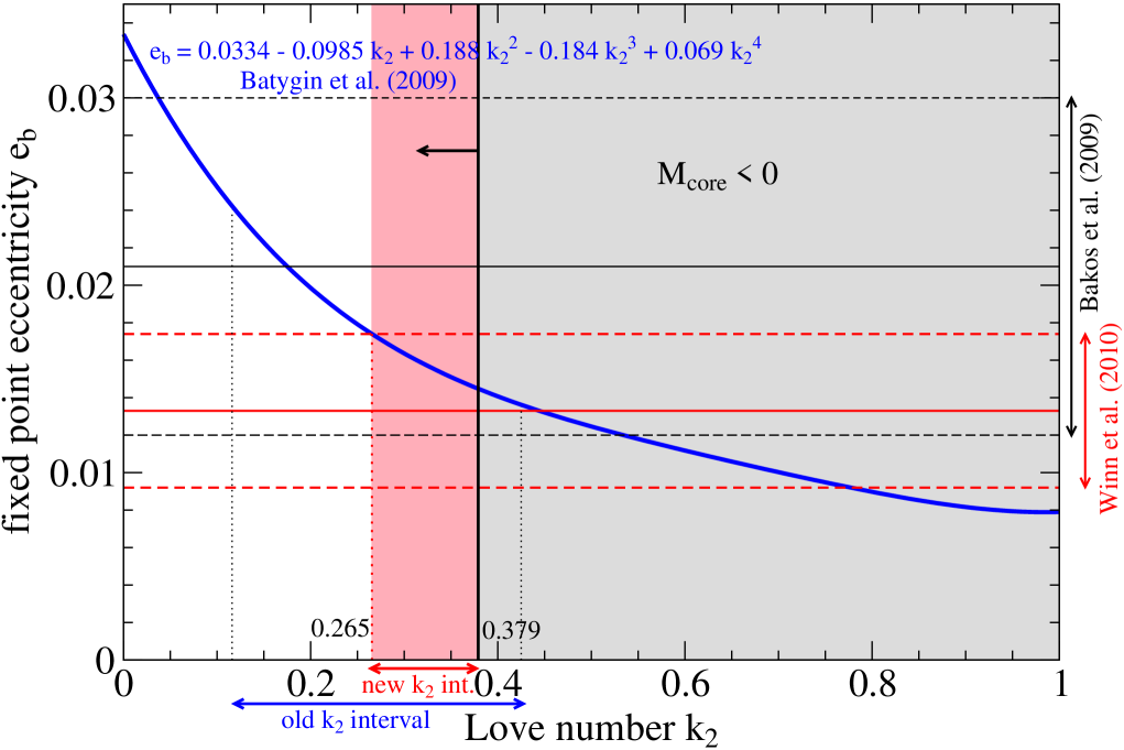
Figure 1: Relation between the fixed point eccentricity $e_{b}$ and the Love number $k_{2}$. The blue line shows the fourth order polynomial fit from Batygin et al. (2009). Different eccentricity measurements from Bakos et al. (2009) and Winn et al. (2010) are plotted in black and red, respectively, with solid lines showing the mean value of the measured eccentricity and dashed lines showing the error bars. The black dotted lines indicate the $k_{2}$ interval inferred from Batygin et al. (2009) based on the eccentricity measurement from Bakos et al. (2009), in the figure also referred to as old $k_{2}$ interval. The gray shaded area marks a region of $k_{2}$ values not possible for models of HAT-P-13b. The vertical black solid line ($M_{\mathrm{core}}=0$) shows the maximum possible $k_{2}$ value we found based on our interior modeling (see §4 for details). Combining the information of the $e_{b}$-$k_{2}$-relation from Batygin et al. (2009), the new eccentricity measurement from Winn et al. (2010), and our interior modeling, we find a new $k_{2}$ interval ranging from 0.265 – 0.379 (rosy shaded).

Based on the eccentricity measurement from Bakos et al. (2009), BBL found an allowed interval for $k_{2}$ of 0.116 – 0.425. This result also includes information from their interior modeling, which is why the limits of the interval are not equal to the intersections of their fourth order polynomial fit and the error bars of the eccentricity measurement. Winn et al. (2010) found a significantly smaller eccentricity. As the eccentricity gets smaller, the resulting $k_{2}$ must become larger. As a consequence, the lower limit of the $k_{2}$ interval is raised to 0.265. To find the upper limit, we make use of our interior models. We find the most homogeneous model of HAT-P-13b at a maximum $k_{2}$ of 0.379. At this point the core mass vanishes and there are no solutions beyond that $k_{2}$ value (for details see §4). This upper limit is also insensitive to variations in mass and radius within the observational error bars (see § 4.2).

By combining the information of the fourth order polynomial fit from BBL, the new eccentricity measurement from Winn et al. (2010), and our interior models, we derived a new $k_{2}$ interval of $0.265<k_{2}<0.379$. It can be expected that this smaller region of allowed $k_{2}$-values will significantly narrow the allowed range of solutions for the interior of HAT-P-13b.

3.3 Model assumptions

For our models we use the mean values for the mass and radius of HAT-P-13b (Bakos et al. 2009):

$$M_{\mathrm{p}}=0.853\,\mathrm{M}_{\mathrm{J}}=271\,\mathrm{M}_{\oplus}\quad,$$

$$R_{\mathrm{p}}=1.281\,\mathrm{R}_{\mathrm{J}}=14.35\,\mathrm{R}_{\oplus}\quad.$$

The uncertainties introduced by the error bars in mass and radius are discussed in § 4.2. We assume a two-layer structure, consisting of a rocky core and one homogeneous envelope of hydrogen, helium and metals. It is not necessary to consider three-layer models in this work because they are within the range of solutions confined by the two-layer models (see §4 for a discussion). We set the helium abundance in the envelope to the solar value $Y=0.27$ (Bahcall et al. 1995). The amount of heavy elements $Z$ was varied from $Z=0$, which gives a model with the biggest possible core when the other parameters are fixed, to a maximum value where the core vanishes.

Due to the proximity to its star, the temperature profile of HAT-P-13b is likely to be strongly influenced by the radiation of the star. The various processes in an exoplanet’s atmosphere influencing its temperature are very complex and beyond the scope of this work. As we aim to study the effects of input parameters important for planet modeling on the structure and Love number of a planet, we vary the envelope temperature within the widest possible range, even though extremely cold or hot models may be unrealistic. For HAT-P-13b we change the 1 kbar temperatures from 3800 to 9000 K. $T_{1\,\mathrm{kbar}}=3800$ K gives the most homogeneous planet with zero core mass and models with $T_{1\,\mathrm{kbar}}>9000$ K would have $k_{2}$ values smaller than the BBL-interval (see also §4). In the outermost layer of the planet from 1 bar to 1 kbar we assume the temperature profile to be either adiabatic or isothermal. This is supposed to account for the uncertainty of how the star’s radiation influences the outer envelope of the planet. As the planet is very close to its star, it is likely that there will be an isothermal layer to some extent (Fortney et al. 2007). In every case, for pressures $P>1$ kbar the planet is adiabatic.

In addition, we compute a model series that is consistent with the nongray model atmospheres from Fortney et al. (2007) in order to further pin down the outer boundary condition. Based on their pressure-temperature profiles of Jupiter-like planets around Sun-like stars (Fig. 3 in Fortney et al. 2007), we interpolated a model atmosphere for HAT-P-13b, assuming that the incoming energy flux remains constant: $L_{*}/(4\pi a^{2})=\mathrm{const.}$, where $L_{*}$ is the stellar luminosity and $a$ is the planet’s semi-major axis. Our interpolation yields $T_{1\,\mathrm{bar}}=2080$ K as new outer boundary condition. It further showed that an isothermal layer may reach down to $P_{\mathrm{ad}}\sim 100$ bar. Our interpolated model atmosphere is in agreement with an atmosphere model specifically calculated for HAT-P-13b, using the methods of Fortney et al. (2007). The thickness of the isothermal layer is a variable parameter (influenced by the age of the planet). Hence, in our model series based on the model atmosphere, we vary $P_{\mathrm{ad}}$ as a free parameter while keeping $T_{1\,\mathrm{bar}}$ fixed at 2080 K.

Our modeling procedure constitutes an improvement compared to the modeling done by Batygin et al. (2009) because we do not approximate the core material by a constant density and we include the effects of different temperatures and temperature profiles in the atmosphere. This allows us to draw some general conclusions about the capability of $k_{2}$ to constrain interior models of extrasolar giant planets.

4 Results

4.1 Love number, metallicity, and core mass

We present in Figs. 2 and 3 results for the calculated core mass, $k_{2}$, and envelope metallicity. The area between an adiabatic and isothermal line of the same 1 kbar temperature accounts for the uncertainty about the outer temperature profile as the thickness of a potential isothermal layer is not known. Also shown are the models based on our model atmosphere with an isothermal layer of 2080 K, reaching down to 1 (fully adiabatic), 5, 10, 50, or 72 bar, where the core disappears. In Fig. 2, the line connecting zero metallicity fully adiabatic models separates the region of all possible planetary models from the prohibited area which is not accessible for models of HAT-P-13b.

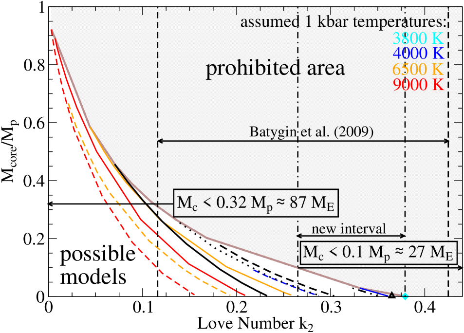
Figure 2: Love numbers $k_{2}$ and core masses of two-layer models of HAT-P-13b for different 1 kbar temperatures (color coded). For pressures $<1$ kbar the temperature profile is either adiabatic (colored solid) or isothermal (colored dashed). The metallicity increases along a line, reaching its maximum value for $M_{\mathrm{core}}/M_{\mathrm{p}}=0$. The zero metallicity line for fully adiabatic models (brown solid) separates the region of all possible planetary models (white) from the prohibited area (light gray). Vertical black dashed lines indicate the allowed interval for $k_{2}$-values derived by BBL. Based on that interval we find a maximum possible core mass of $0.32\,M_{\mathrm{p}}\approx 87$ M_⊕. Our new $k_{2}$ interval is shown with vertical black dot-dashed lines. It lowers the uncertainty of the planet’s core mass down to $0.1\,M_{\mathrm{p}}\approx 27$ M_⊕. The other black lines show our models that are based on our model atmosphere with a fully adiabatic envelope (solid black) and $P_{\mathrm{ad}}$ of 5 bar (dotted), 10 bar (dashed black), 50 bar (dot-dashed black), and 72 bar (black triangle).

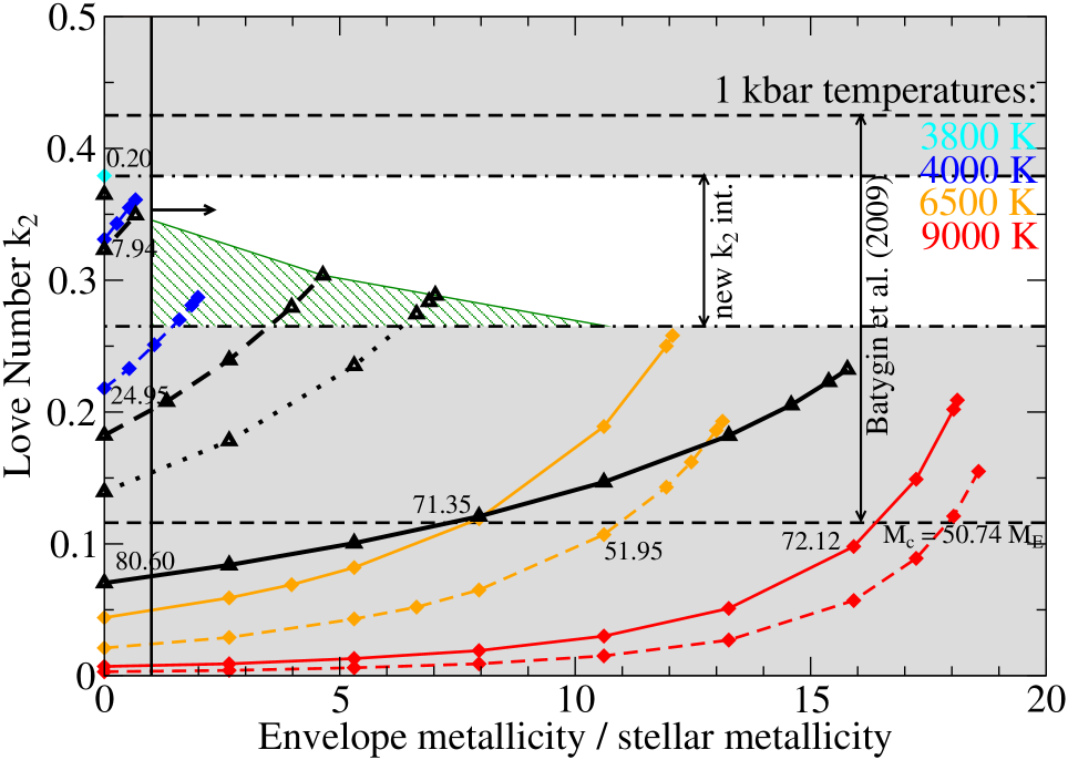
Figure 3: Love numbers $k_{2}$ as a function of the envelope metallicity. Shown are the same models as in Fig. 2. The numbers close to some models give the core mass in M_⊕. The shaded areas demonstrate how models can be ruled out by taking into account the $k_{2}$ intervals and assuming that the envelope metallicity is at least the stellar metallicity. Considering the information from the model atmosphere the favored models reduce to the green shaded area.

A general trend that can be seen in Fig. 2 and 3 is that the Love number $k_{2}$ increases as more metals are put in the envelope. This is the result of $k_{2}$ being a measure of the level of central condensation of an object. Since the total mass of the planet must always be $M_{\mathrm{p}}$, the enrichment of the envelope with metals leads to a decrease in core mass. A smaller core and higher metal content in the envelope means that the planet is more homogeneous, which is why the Love number grows. The maximum metallicity is reached when the core of the planet vanishes. This marks the maximum possible Love number of a planet for a given temperature.

The temperature itself also has a significant influence on the metallicity, core mass, and consequently Love number of the planet. Higher temperatures reduce the Love number $k_{2}$. The higher the envelope temperature, the lower its density. Low densities in the envelope require a more massive core in order to ensure mass conservation. High envelope temperatures thus lead to a strong central condensation, reflecting in a small Love number. For HAT-P-13b we find a minimum 1 kbar temperature of 3800 K for fully adiabatic models. At this low temperature the zero metallicity envelope is so dense that the core is almost vanished ($M_{\mathrm{core}}=0.2$ M_⊕). Hence, there is no enrichment of heavy elements possible in the envelope. At this temperature maximum homogeneity is reached. That translates into a maximum possible Love number for HAT-P-13b of $k_{2}=0.379$, well below the upper limit given by the BBL-interval. At high temperatures, on the other hand, the density in the envelope is low enough to enable the existence of massive cores. That creates the possibility to enrich the envelope with metals. For instance, at $T_{\mathrm{1\,kbar}}=9000$ K the core disappears at an envelope metallicity as high as 70%. The big cores of the hot models lead to very small Love numbers and tend to lie outside of the BBL-interval.

We note that models with an isothermal atmosphere generally yield smaller Love numbers than their adiabatic counterparts, because they are overall hotter.

As is obvious from Fig. 2 and 3 not all calculated models are placed in the BBL-interval or even in our narrower new $k_{2}$ interval, which means some of the models can be ruled out. The hot and metal poor models cannot fulfill the BBL-interval. Our new $k_{2}$ interval also rules out the metal rich hot models and only leaves us with the colder models.

Further constraints can be made by taking into account model atmospheres in order to get more information about the planet’s outer temperature profile. Our model atmosphere yields a 1 bar temperature of 2080 K. An isothermal layer of $P_{\mathrm{ad}}>3$ bar is required to produce solutions in our new $k_{2}$ interval.

Another point we can take into account is that planets form out of the same cloud of gas as their host star. Hence, it is reasonable to assume that the planet’s bulk metallicity is at least the stellar metallicity. Of course, a planet may also be enriched in metals due to capture of planetesimals during formation. Enhanced bulk metallicities for extrasolar giant planets over their parent star values were indeed found (Miller & Fortney 2011). We use this argument to also rule out interior models that have less than stellar metallicity (see Fig. 3). Here we can approximate the bulk metallicity with the envelope metallicity as the disputable models have such small cores that most of the planet’s metals are in the envelope. This leaves us only with very few models for the interior of HAT-P-13b, where we favor the ones compatible with the model atmosphere. Combining all the pieces of information, we can conclude from Fig. 3 that HAT-P-13b has an isothermal outer layer with a temperature of 2080 K that may reach down to 3 – 44 bar. Models with isothermal layers that extend to higher pressures have such small cores that their envelope metallicity cannot exceed stellar metallicity. Consequently, our models with $P_{\mathrm{ad}}\geq 50$ bar are ruled out. The envelope metallicity of the allowed models is 1 – 11 times the stellar metallicity. Also, the bulk metallicity cannot exceed this limit as $M_{\mathrm{core}}<27$ M_⊕.

In order to give a better overview of the different boundary conditions used we plot in Fig. 4 P–T profiles of acceptable and some unacceptable models. Those with $T_{\mathrm{1\,kbar}}<4000$ K and $T_{\mathrm{1\,kbar}}>6500$ K are too cold or too hot, respectively, and hence not shown in the plot. We find an area that roughly constrains the P-T-conditions near the atmosphere that produce acceptable models. In addition, a model also needs to have a high enough envelope metallicity in order to be acceptable. For example, our structure models compatible with our model atmosphere with $T_{\mathrm{1\,bar}}=2080$ K and an isothermal layer down to 10 bar lie in the favored area marked by Fig. 4. However, models of this kind with $Z=0$ are not acceptable whereas models with a high enough envelope metallicity are, compare also to Fig. 3.

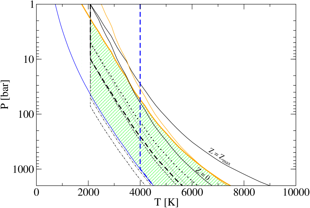
Figure 4: P–T profiles near the atmosphere of acceptable and unacceptable models. Colors and line styles are the same as in Figs. 2 and 3. For lines with same color and style, models with $Z=0$ and $Z=Z_{\mathrm{max}}$ are shown. Thick lines indicate acceptable models; compare these also to Fig. 3. The green shaded area marks the P–T regime for acceptable models. However, models in this regime are only acceptable when they also have a large enough amount of metals in their envelopes.

A very important parameter describing the interior of a planet is its core mass. This quantity is of interest because it may give a hint on the formation history of the planet. Figure 2 shows that the relationship between a $k_{2}$ value and a core mass is non-unique. If, for instance, $k_{2}=0.2$ it could either be a very hot $T_{\mathrm{1\,kbar}}=9000$ K, metal rich planet with a very small core or a lower temperature $T_{\mathrm{1\,kbar}}=6500$ K one with a core constituting 10% of the planet’s total mass. The only information that can be concluded is a maximum possible core mass, given by the line consisting of the adiabatic zero metallicity models. The maximum possible core mass of HAT-P-13b is given by the intersection of this line with the lower $k_{2}$ boundary, yielding $M_{\mathrm{core}}<0.32\,M_{\mathrm{p}}\approx 87$ M_⊕ for the BBL-interval. Taking into account our new $k_{2}$ interval lowers the uncertainty of the planet’s core mass down to $M_{\mathrm{core}}<0.1\,M_{\mathrm{p}}\approx 27$ M_⊕.

In principle, the area under each curve can be filled up with three-layer models (not shown in Fig. 2). Every redistribution of metals in the envelope would either result in a stronger central condensation (smaller $k_{2}$) or, if central condensation is kept constant, require a transport of material from the core to the envelope reducing the core mass. As a result of this degeneracy introduced by a discontinuity in the envelope (see also Kramm et al. 2011) it is only possible to determine a maximum possible core mass. Further narrowing of the maximum core mass could also be achieved with a more detailed measurement of the eccentricity of HAT-P-13b as that would lead to a smaller $k_{2}$ interval.

Finally, from all the interior models we presented here, we favor the ones with $T_{\mathrm{1\,bar}}=2080$ K, an isothermal outer layer of 3 – 44 bar, and an envelope metallicity of $1<Z/Z_{*}<11$ because they (i) are placed in our new $k_{2}$ interval, (ii) are consistent with the model atmospheres from Fortney et al. (2007), and (iii) have an envelope and bulk metallicity that is above the stellar metallicity. Assuming these parameters are ”correct” for HAT-P-13b, the planet would have a core mass of 27 M_⊕ or less. For comparison, Jupiter models from Fortney & Nettelmann (2010) predict $M_{Z,\mathrm{tot}}=15-38$ M_⊕, $M_{\mathrm{core}}=0-10$ M_⊕ and $Z_{\mathrm{p}}=4-12\,Z_{\odot}$.

4.2 Mass and radius uncertainties

We now investigate the effect of the measurement uncertainties for the mass and radius of HAT-P-13b. For that purpose, we varied the mass and radius within the $1\sigma$ error-bars to obtain different mean densities. As an example, we only look at models consistent with our model atmosphere and $P_{\mathrm{ad}}=1$ and 50 bar because all other valid models are bounded by these and react the same way on mass-radius variations.

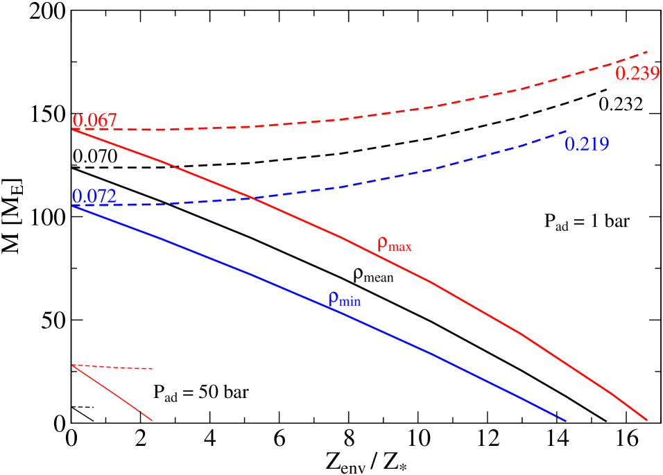
Figure 5: Core mass (solid lines) and total mass of metals (dashed lines) as a function of envelope metallicity for different mean densities according to the measurement uncertainties in mass and radius. The numbers are the Love numbers $k_{2}$ for zero and maximum possible metallicity in the envelope. Shown are only models compatible with our model atmosphere ($T_{\mathrm{1\,bar}}=2080$ K) for $P_{\mathrm{ad}}=1$ bar and $P_{\mathrm{ad}}=50$ bar.

Figure 5 shows the effect on core mass and metal enrichment. The uncertainty in mean density results in an uncertainty of about $\pm 20$ M_⊕  in core mass and mass of metals. For a given core mass, the envelope metallicity can vary up to $\pm 3\,Z_{*}$.

There is little effect on the Love number $k_{2}$. In Fig. 2, the line separating the prohibited area from the possible models consists of zero-metallicity models. Since for $Z_{\mathrm{env}}=0$ the Love number $k_{2}$ only varies by about $\pm 0.003$, only a minor shift of this line can be expected so that all the conclusions drawn for the fiducial $M_{\mathrm{p}}$ and $R_{\mathrm{p}}$ values remain valid also for other mean densities within the error bars.

4.3 Estimating the tidal $Q$ value

With $R_{\mathrm{p}}=1.281$ R_J HAT-P-13b has a large radius given its mass and age. This implies it possesses an interior energy source, like many other Hot Jupiter planets. Given its eccentric orbit, this energy source could have a strong contribution due to tidal heating.

Based on our analysis of $k_{2}$ and our interior models we found that the adiabatic transition is between 3 and 44 bar. We ran atmosphere models to estimate what values of the intrinsic temperature ($T_{\mathrm{int}}$) these would correspond to. At the adiabatic transitions of 3 and 44 bar we found $T_{\mathrm{int}}=750$ and 275 K, respectively. This also gives us the intrinsic luminosity $L_{\mathrm{int}}$. Assuming $L_{\mathrm{int}}$ is provided only by tidal heating, we estimated $Q$ with the following relation (Miller et al. 2009)

$$L_{\mathrm{int}}\approx P_{\mathrm{t}}=\frac{63}{4}\left[(GM_{*})^{3/2}\left(\frac{M_{*}R_{\mathrm{p}}^{5}e_{b}^{2}}{Q}\right)\right]a^{-15/2}\quad.$$ (5)

This gives us a lower limit on the $Q$ value of HAT-P-13b since tidal heating might not be the only interior energy source. There could be other effects contributing to $L_{\mathrm{int}}$, for instance Ohmic dissipation (Batygin & Stevenson 2010).

Our estimates of the lower limit on $Q$ for the different eccentricity measurements are displayed in Tab. 1. For comparison, Jupiter’s $Q$ value has been calculated to be between $10^{5}$ and $10^{6}$ (Goldreich & Soter 1966).

Table 1: Lower limits for the tidal $Q$ value of HAT-P-13b for different eccentricity measurements and intrinsic temperatures (resulting from the allowed extension of the isothermal layer in the planet’s atmosphere).

$T_{\mathrm{int}}$ [K]	$e_{b}=0.021$	$e_{b}=0.0133$
	(Bakos et al. 2009)	(Winn et al. 2010)
275 (44 bar)	176 485	70 790
750 (3 bar)	3 190	1 280

5 Discussion

5.1 Comparison with previous results

In addition to an allowed $k_{2}$-interval, Batygin et al. (2009) also provided a set of possible interior models of HAT-P-13b that give $k_{2}$ values within the given interval. These models range in core mass from 0 to 120 M_⊕. However, for the given BBL-interval we find a maximum possible core mass that is significantly smaller ($\approx 87$ M_⊕). This difference is a result of different model assumptions. The models of Batygin et al. (2009) all have cores with constant densities of 7-12 g/cm³ (Batygin, pers. comm.), resembling water cores. In contrast, the models presented in this work were calculated using a compressible rock EOS (Hubbard & Marley 1989), increasing the densities in the cores up to 12-40 g/cm³. As a consequence of the lower and constant core densities in the BBL models, a core of a specific mass requires a larger radius than a core of the same mass in our models. This results in a greater Love number than our models with the same core mass. That is why our models need smaller core masses in order to fall in the allowed $k_{2}$-interval. Models of HAT-P-13b in this work with a core mass of 120 M_⊕would have a smaller $k_{2}$ than the lower $k_{2}$-boundary of the BBL-interval. Hence, the different maximum core masses in this work and in Batygin et al. (2009) arise from the different core EOS used. This shows the major influence of the EOS. In our example here, the different core EOS cause an uncertainty of about 28% in the maximum possible core mass.

5.2 The eccentricity issue

As mentioned before (see § 3.2) the eccentricity is crucial for determining an allowed $k_{2}$-interval. We used the results from BBL to obtain a new $k_{2}$ interval from another eccentricity measurement (Winn et al. 2010). Our new interval, ranging from 0.265 to 0.379 is significantly smaller than the one previously used by BBL ($0.116<k_{2}<0.425$). This allowed for a more precise estimate of a maximum possible core mass ($M_{\mathrm{core}}<27$ M_⊕).

It of course has to be kept in mind that the ultimate significance of this new eccentricity value (and deduced $k_{2}$) is unclear. Other effects like the stellar jitter produce a large uncertainty on the eccentricity measurement of the inner planet, as recently pointed out by Payne & Ford (2011).

One way to help to constrain the eccentricity would be a detection of the occultation (secondary eclipse) of the planet (for instance, with Spitzer). The timing of the occultation can be used to place a strong constraint on $e\cos\omega$, where $e$ is the orbital eccentricity and $\omega$ is the longitude of periastron (Charbonneau et al. 2005). Observations to determine $e\cos\omega$ for HAT-P-13b are currently being made (Harrington & Hardy, pers. comm.).

6 Summary & Conclusions

In this work, we presented new interior models of the transiting Hot Jupiter HAT-P-13b with the aim of showing to what extent interior models of extrasolar giant planets can be constrained by using the tidal Love number $k_{2}$ in addition to the known observables mass and radius. We also varied the envelope temperature and metallicity in order to demonstrate the uncertainties imposed on the inferred interior models.

One main result of our work is that based on the Love number $k_{2}$ one cannot draw a conclusion on the precise core mass of the planet. Only a maximum possible core mass can be inferred which is given by adiabatic zero-envelope-metallicity models. Taking into account the allowed $k_{2}$ interval ($0.116<k_{2}<0.425$) derived from Batygin et al. (2009), we find a maximum value for HAT-P-13b’s core mass of 87 M_⊕. Further radial velocity observations from Winn et al. (2010) gave a new value for the planet’s eccentricity, allowing us to construct a new $k_{2}$ interval of $0.265<k_{2}<0.379$. With this smaller interval we were able to constrain the core mass of HAT-P-13b further down to 27 M_⊕.

We also showed the influence of the envelope’s temperature and metallicity. The coldest possible model defines a maximum possible value for $k_{2}$ as this is the most homogeneous model. For HAT-P-13b we find $k_{2,\mathrm{max}}=0.379$. This is well below the upper $k_{2}$ limit from Batygin et al. (2009).

As our analysis showed, the temperature and metallicity of the planet’s envelope are important parameters whose knowledge would significantly increase the effectiveness of constraining the planet’s interior with the Love number $k_{2}$. We therefore calculated a model series based on a theoretical model atmosphere from Fortney et al. (2007). Models of this kind have $T_{\mathrm{1\,bar}}=2080$ K and fall in our new $k_{2}$ interval if they have an outer isothermal layer with $3\,\mathrm{bar}<P_{\mathrm{ad}}<44\,\mathrm{bar}$. With this result we also estimated lower limits of the tidal $Q$ value of HAT-P-13b.

Based on our analysis and the applicability of the tidal fixed point theory we can rule out the majority of the calculated models. Assuming our new $k_{2}$-interval, we note that hot models with $T_{1\,\mathrm{kbar}}>6500$ K can be ruled out (compare Fig. 3). On the other hand, the very cold models with $T_{\mathrm{1\,kbar}}<4000\,$K are unlikely because they have a metallicity that is smaller than stellar. We favor models with $T_{\mathrm{1\,bar}}=2080$ K, an isothermal outer layer of 3 – 44 bar, and an envelope metallicity of $1<Z/Z_{*}<11$ because they (i) are placed in our new $k_{2}$ interval, (ii) are consistent with the model atmospheres from Fortney et al. (2007), and (iii) have an envelope metallicity that is above the stellar metallicity. Assuming these conditions really apply for HAT-P-13b the planet would have a core mass of 27 M_⊕ or less. Given the calculated tidal $Q$, if HAT-P-13b turns out to have a small core and an envelope enrichment similar to Jupiter, it could represent a Jupiter-like extrasolar planet.

By comparing with the previous results from Batygin et al. (2009) we have seen that the core EOS affects the core mass and Love number, resulting into a difference of about 28% in the prediction of a maximum possible core mass of HAT-P-13b.

As pointed out in §3.2, the eccentricity of the inner planet is a crucial parameter because it determines the Love number $k_{2}$. The value of the eccentricity is still uncertain. We analyzed the consequences of an $e_{b}=0.021\pm 0.009$ (Bakos et al. 2009) and $e_{b}=0.0133\pm 0.0041$ (Winn et al. 2010).

Finally, despite the uncertainty of the inner planet’s eccentricity it is still unclear whether the tidal fixed point theory from Mardling (2007) can really be applied to HAT-P-13b. Further observations are necessary to prove the co-planarity and apsidal alignment configuration of the system. Also, TTV measurements could provide clues about the existence of other long-period companions in the system.

Appendix A Applicability of the tidal fixed point theory

The analysis in this work is based on the assumption that the tidal fixed point theory of Mardling (2007) can be applied in order to extract a $k_{2}$ value from the inner planet’s eccentricity. For that purpose the planetary system has to fulfill the requirements mentioned in §3.1. Yet unproven and crucial to the evolution into the tidal fixed point is the co-planarity of the HAT-P-13 system. In fact, if the orbits of planet b and c are mutually inclined, the system will not evolve to the tidal fixed point. Instead it will relax to a limit cycle in $e_{b}$ - $\eta$ parameter space where the eccentricity of the inner planet $e_{b}$ and the angle between the periapse lines $\eta$ oscillate (Mardling 2010). In that case the Love number $k_{2}$ of the inner planet can not be determined unambiguously. In particular, Mardling (2010) shows that the analysis of Batygin et al. (2009) and hence the inferred $k_{2}$-interval is only valid if the mutual inclination of planets b and c is less than about 10^∘.

A direct estimate of the mutual inclination $\Delta i$ would be possible by observing planet c in transit and measuring the Rossiter-McLaughlin effect. A transit of HAT-P-13c was predicted to occur on April 28, 2010 (Winn et al. 2010). However, such a transit could not be observed. The multi-site campaign by Szabó et al. (2010) revealed that a transit of HAT-P-13c can be excluded with a significance level from 65% to 72%. Yet, a close to co-planar configuration cannot be ruled out. The transit probability of HAT-P-13c is at most 8.5% for a mutual inclination of the two planets of 8^∘ and decreases to zero for inclinations $\lesssim 4^{\circ}$ (Beatty & Seager 2010). Another reason why the campaign of Szabó et al. (2010) could not detect a transit may be that they only observed for 5 days. The orbital parameters (eccentricity and period) of the outer planet are not well constrained due to the effect of the unknown stellar jitter, which translates into large uncertainties about the predicted transit times of planet c, making it necessary to observe over a wide range of nights— $\sim 3$ weeks (Payne & Ford 2011).

Support for the hypothesis of co-planarity of the HAT-P-13 system comes from the study of the Rossiter-McLaughlin effect to determine the stellar obliquity $\Psi_{*,b}$. Winn et al. (2010) note that there is an indirect connection between $\Psi_{*,b}$ and $\Delta i$: a large $\Delta i$ would lead to nodal precession of b’s orbit around c’s orbital axis, causing periodic variations in $\Psi_{*,b}$. As a consequence, it would be unlikely to observe a low value of $\Psi_{*,b}$ unless $\Delta i$ is also small. At any rate, only the sky-projected angle $\lambda$ can be measured (not the true obliquity $\Psi_{*,b}$) which makes it still impossible to draw firm conclusions about $\Delta i$. Winn et al. (2010) find a small $\lambda=1.9\pm 8.6\,{\rm deg}$, suggesting that planet b’s orbital angular momentum vector is well-aligned with the stellar spin vector. This also increases the likelyhood that the orbits of planets b and c are co-planar.

Payne & Ford (2011) also suggest a method to determine the mutual inclination between planets b and c with the help of transit timing variations (TTV). In particular, they show that systems with $\Delta i\sim 0^{\circ}$ and $\Delta i\sim 45^{\circ}$ result in significantly different TTV profiles which can easily be distinguished. In fact, HAT-P-13b has been subject to a TTV campaign. Pál et al. (2011) detected TTV in the order of 0.01 days which ’suddenly’ occured during their observations in December 2010 and January 2011 while in the first three years of observations of HAT-P-13b there seemed to be a lack of TTV. If it is a periodic process, it should have a period of at least $\sim 3$ years, making it unlikely to be caused by HAT-P-13c. Hence, Pál et al. (2011) conclude that the measured TTV may be the result of perturbations of another long-period companion. Interestingly, Winn et al. (2010) also point to the possibility of an additional body d in the system as their models of two Keplerian orbits give an unacceptable fit to the RV data while a model assuming a third companion with a longer orbital period is successful. Furthermore, thinking about the origin of the HAT-P-13 system, Mardling (2010) suggests that the system originally contained a third planet which was later scattered out of the system.

Given all these issues, to our current knowledge it seems impossible to say whether HAT-P-13b is really subject to the tidal evolution into the tidal fixed point like envisioned by Mardling (2007). Further observations are necessary to pin down the mutual inclination of the planets and to prove or disprove the existence of another companion in the system.