Nanoshells as a high-pressure gauge analyzed to 200 GPa

Abstract

In this article we present calculations which indicate that nanoshells can be used as a high pressure gauge in Diamond Anvil Cells (DACs). Nanoparticles have important advantages in comparison with the currently used ruby fluorescence gauge. Because of their small dimensions they can be spread uniformly over a diamond surface without bridging between the two diamond anvils. Furthermore their properties are measured by broad band optical transmission spectroscopy leading to a very large signal-to-noise ratio even in the multi-megabar pressure regime where ruby measurements become challenging. Finally their resonant frequencies can be tuned to lie in a convenient part of the visible spectrum accessible to CCD detectors. Theoretical calculations for a nanoshell with a SiO₂ core and a golden shell, using both the hybridization model and Mie theory, are presented here. The calculations for the nanoshell in vacuum predict that nanoshells can indeed have a measurable pressure-dependent optical response desirable for gauges.However when the nanoshells are placed in commonly used DAC pressure media, resonance peak positions as a function of pressure are no longer single-valued and depend on the pressure media, rendering them impractical as a pressure gauge. To overcome these problems an alternative nanoparticle is studied: coating the nanoshell with an extra dielectric layer (SiO₂) provides an easy way to shield the pressure gauge from the influence of the medium, leaving the compression of the particle due to the pressure as the main effect on the spectrum. We have analyzed the response to pressure up to 200 GPa. We conclude that a coated nanoshell could provide a new gauge for high-pressure measurements that has advantages over current methods.

LABEL:FirstPage1

I Introduction

Recently nanoshellsNS have received a lot of attention because they possess interesting optical properties. Consisting of a dielectric core surrounded by a metallic shell, nanoshells allow surface plasmon polaritons to exist at the interfaces between the layers, resulting in a spectrum with very pronounced absorption and extinction peaks. The position and broadness of these resonance peaks depend on the size, shape and materials of the particles and on the surrounding medium. This versatility and sensitivity make nanoshells excellent probes in different fields, ranging from cancer ablationcancer and biosensorsbiosensor to surface enhanced raman spectroscopy applicationssers and plasmonicsPlasmonics . In this paper we investigate the usefulness of nanoshells in the field of high-pressure physics, and more precisely Diamond Anvil Cell (DAC) pressure measurementsDAC . The first theoretical calculations for a spherically symmetric SiO₂-gold nanoshell under pressure (up to 200 GPa) are presented, indicating clear measurable absorption peaks. The main idea behind the use of nanoshells as a pressure gauge is that the size of the nanoshell and the permittivity of the SiO₂ core and medium will change under pressure resulting in a shift of the resonance frequencies. The goal of this paper is to calculate the optical transmission as a function of wavelength for a spatial distribution of noninteracting monodisperse nanoshells.

At the moment there are several pressure gauges used in high-pressure physics. We briefly discuss them and conclude with the advantages of the nanoshell-gauge in comparison with the established methods. The prime and venerable pressure gauge is the shift of the peak of the ruby fluorescence spectrum with pressureRuby ; Rubyscale , excited by laser pumping. In this case micron sized ruby grains are embedded in the pressurization medium. Several problems can arise above a certain pressureRuby error ; Rubyto150GPa : at pressures above 100 GPa diamond fluorescence can become intense and mask the ruby line; ruby grains can be blown away during loading or masked during pressurization; above a few hundred GPa the standard method of pumping the ruby with a green or blue laser line becomes ineffectual as the laser light is absorbed by the diamond anvil. Although some of these problems can be overcomeEggert ; Chen , ruby becomes challenging to use at very high pressure. For cases where the ruby is lost or cannot be observed researchers have used the phonon Raman spectrum of the diamond from the high pressure culet or stressed region of the diamond. This is less precise and has some dependence on the diamond geometryBaer . Another method is to embed a grain of diamond in the pressurization medium, but this also has challenges and limitationsDubrovinskaia . An important gauge is the X-ray spectrum of metal “markers” embedded in the pressurization medium, but this is only useful at synchrotrons. Finally we mention that many of the pressure gauges have problems at high temperatures. The advantages of the nanoshells, which come dispersed in a volatile fluid, is that they can be painted onto the diamond culet in a thin invisible (to the eye) layer so they will not blow out and they cover the entire culet flat so they cannot easily be masked; they should maintain their sensitivity to the highest pressures; optical spectroscopy is easy to implement with a large signal-to-noise ratio, compared to fluorescence or Raman scattering, and will not be masked by fluorescence from the diamonds. We believe that nanoshells will maintain their sensitivity at high temperatures, but this requires further study.

The article is organized as follows. In section II we first review existing theories that can be used to calculate the spectrum and resonance frequencies of a nanoshell. Next, the pressure dependency is taken into account. In section III the results of the calculations are shown for the nanoshell geometry. To overcome some of the problems seen with nanoshells the coated nanoshell is introduced in section IV. Section V contains the conclusions.

II Theory

The optical properties of nanoshells are usually described by either Mie theory or the hybridization model. The hybridization model, developed by Nordlander and co-workersHybri1 , offers a fast-to-evaluate analytical form for the resonance frequencies, but it is only valid for small particles (smaller than ca. a tenth of the wavelength). Mie theoryStratton is valid for all particle sizes but this method is far more time consuming for calculating the peak positions since it does not allow for a closed form analytical formula for the position of the resonance peak. These resonance peak positions have to be numerically derived from the absorption or extinction spectrum.

In this section first both theories will be reviewed. The pressure dependency is taken into account in the last part of this section.

II.1 Hybridization theory

Hybridization theoryHybri1 is a phenomenological approach in which the nanoshell is modeled as a combination of a cavity and a metallic sphere. First the sphere and cavity are studied separately. The free electrons of the sphere are descibed as an incompressible fluid excited by plasmons and the dielectric function is assumed to be that of a Drude metalKittel :

$$\varepsilon_{s}\left(\omega\right)=\varepsilon_{b}-\frac{\omega_{pl}^{2}}{\omega^{2}},$$ (1)

where $\varepsilon_{b}$ indicates the background permittivity and $\omega_{pl}$ the bulk plasma frequency of the metal.

In a second step the resonance frequencies of the cavity and the sphere are hybridized due to the coupling between the cavity and the sphere modes, very similar to the hybridization of molecular orbitals. This results in a closed formula for the resonance frequenciesHybri2 :

$$\omega_{L,\pm}^{2} =\frac{\omega_{pl}^{2}}{\beta}\left(\left(L+1\right)^{2}\varepsilon_{m}+2L\left(L+1\right)\varepsilon_{b}+L^{2}\varepsilon_{c}+L\left(L+1\right)\left(\varepsilon_{m}-2\varepsilon_{b}+\varepsilon_{c}\right)x^{2L+1}\right.$$ (2)

$$\pm\left\{\left[L^{2}\varepsilon_{c}-\left(L+1\right)^{2}\varepsilon_{m}+L\left(L+1\right)\left(\varepsilon_{m}-\varepsilon_{c}\right)x^{2L+1}\right]^{2}\right.$$

$$\left.\left.+4L\left(L+1\right)\left[\left(L+1\right)\varepsilon_{m}+L\varepsilon_{c}\right]^{2}x^{2L+1}\right\}^{1/2}\right)$$

with:

$$\beta =2\left\{\left[\left(L+1\right)\varepsilon_{b}+L\varepsilon_{c}\right]\left[\left(L+1\right)\varepsilon_{m}+L\varepsilon_{b}\right]\right.$$ (3)

$$\left.+L\left(L+1\right)\left(\varepsilon_{b}-\varepsilon_{c}\right)\left(\varepsilon_{m}-\varepsilon_{b}\right)x^{2L+1}\right\},$$

where $\varepsilon_{c}$, $\varepsilon_{b}$ and $\varepsilon_{m}$ are the permittivities of the core, the background of the shell (see formula $\left(\ref{Drude}\right)$) and the medium respectively, $L$ is the orbital quantum number and $x=R_{c}/R_{s}$ is the ratio between the core $\left(R_{c}\right)$ and shell $\left(R_{s}\right)$ radii.

II.2 Mie theory

Mie theory is used to solve the Maxwell equations in systems with spherical symmetryStratton . It allows the calculation of the absorbed, scattered and total cross section for an incident beam of radiation as a function of frequency. The nanoshell is modeled as two concentric spherical spheres. For this case the results originally derived by Mie for a single spherical interface were worked out by Aden and KerkerAdenKerker . The coated nanoshell, which will be introduced later, is modeled by three concentric spheres. Extending Mie theory to three concentric spheres, although not available in literature, does not provide any new problems in comparison with the two concentric sphere case solved by Aden and Kerker. The final expressions for the electromagnetic fields in and around the coated nanoshell, as well as the scattering and absorption cross section, are given in the appendix. From the resulting total cross section the resonance frequencies can be determined numerically.

For this method the input parameters are again the sizes and permittivities of the shells. In analogy with the hybridization model we used the Drude dielectric function in Mie theory to describe the permittivity of the metal shell.

II.3 Pressure dependency: equation of state

Applying a pressure $P$ to a nanoshell will lead to a change of the volume of the core $V_{c}\left(P\right)$ and the shell $V_{s}\left(P\right)$. These changes can be calculated using the Vinet equation of state (EOS)VinetEOS :

$$P=3K_{0}\frac{1-\left(\frac{V}{V_{0}}\right)^{1/3}}{\left(\frac{V}{V_{0}}\right)^{2/3}}\exp\left\{\frac{3}{2}\left(K_{1}-1\right)\left[1-\left(\frac{V}{V_{0}}\right)^{1/3}\right]\right\},$$ (4)

which gives the relation between the pressure $P$ and the relative volume change $V/V_{0}$ with respect to a reference volume $V_{0}$ of a material at a certain temperature. Here $K_{0}$ and $K_{1}$ are material constants for which the values used in this article are presented in table 1.

Table 1: The material properties used in the pressure calculations of the nanoshell. Parameters $K_{0}$ and $K_{1}$ are valid up to $580$ GPa for gold and $150$ GPa for amorphous silicon according to resp. ref. K0K1enV0Au and ref. K0K1enV0SiO2 . The last column indicates the relative permittivity at ambient pressure. The permittivity indicated for gold is the bulk permittivity $\varepsilon_{b}$ as defined in equation 1.

Material	$\mathbf{K}_{0}$ $\left(\text{GPa}\right)$	$\mathbf{K}_{1}$	$\varepsilon$
Amorphous SiO2	$329$K0K1enV0SiO2	$4.1$K0K1enV0SiO2	$2.0449$PermSIO2
Au	$167$K0K1enV0Au	$5.94$K0K1enV0Au	$6.9$DrudeBronbackground

Using the Vinet EOS one can calculate the size change of the nanoshell under pressure where $V_{0}$ has been taken as the original volume at zero pressure. Under pressure the nanoshell will be compressed resulting in a different core and shell radius and a different bulk plasma frequency. These changes can be calculated from:

$$R_{c}\left(P\right) =R_{c}\left(0\right)\left(\frac{V_{c}\left(P\right)}{V_{c}\left(0\right)}\right)^{1/3},$$ (5)

$$R_{s}\left(P\right) =\left\{R_{s}^{3}\left(0\right)\left(\frac{V_{s}\left(P\right)}{V_{s}\left(0\right)}\right)+R_{c}^{3}\left(0\right)\left[\left(\frac{V_{c}\left(P\right)}{V_{c}\left(0\right)}\right)-\left(\frac{V_{s}\left(P\right)}{V_{s}\left(0\right)}\right)\right]\right\}^{1/3},$$ (6)

$$\omega_{pl}^{2}\left(P\right) =\frac{n\left(P\right)e^{2}}{\varepsilon_{0}m}=\left(\frac{V_{s}\left(0\right)}{V_{s}\left(P\right)}\right)\omega_{pl}^{2}\left(0\right),$$ (7)

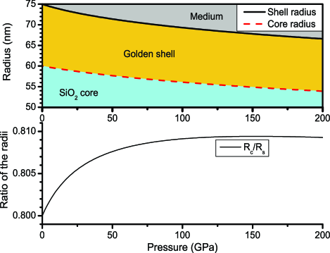
Figure 1: The behavior of the sizes of the nanoshell under pressure. The top panel presents the radii of the core and shell as a function of pressure. Notice that the golden shell will be compressed more than the core until about $150$ GPa where the core/shell ratio reaches a maximum. The bottom panel shows this ratio $R_{c}/R_{s}$, which is an important parameter for the optical response. The radii of the nanoshells in this article correspond to the size of commercially available nanoshells.

where $V_{c}\left(P\right)$ and $V_{s}\left(P\right)$ are the volumes of the core and the shell respectively, $n$ is the bulk electron concentration, $e$ is the electron charge, $\varepsilon_{0}$ is the permittivity of vacuum and $m$ is the electron mass. The pressure dependency of the radii is shown in Figure 1 for a nanoshell with $R_{c}=60\operatorname{nm}$ and $R_{s}=75\operatorname{nm}$. When the nanoshell is compressed the electron density will increase and so will the bulk plasma frequency (7). This will also influence the permittivity of the metal since the plasma frequency is an essential part of the Drude dielectric function (see Eq. $\left(\ref{Drude}\right)$).

The pressure and frequency dependency of the permittivity of SiO₂ in the megabar regime remains, to the best of our knowledge, unknown. However it is possible to estimate the pressure dependency from the Vinet EOS using the Clausius-Mossotti relationKittel :

$$\frac{\varepsilon\left(\omega,P\right)-1}{\varepsilon\left(\omega,P\right)+2}=\frac{4\pi}{3}n\left(P\right)\alpha,$$ (8)

where $n\left(P\right)=N/V\left(P\right)$ is the electron density and $\alpha$ the average atomic polarizability, assumed independent of pressure. This relation links the permittivity to the volume of a material. Dividing this equation with the same equation at zero pressure allows us to estimate

$$\varepsilon(\omega,P)=\frac{2\frac{\varepsilon(\omega,0)-1}{\varepsilon(\omega,0)+2}+\frac{V_{c}\left(P\right)}{V_{c}\left(0\right)}}{\frac{V_{c}\left(P\right)}{V_{c}\left(0\right)}-\frac{\varepsilon(\omega,0)-1}{\varepsilon(\omega,0)+2}},$$ (9)

where $V\left(P\right)/V_{0}$ can be calculated from the Vinet EOS $\left(\ref{Vinet EOS}\right)$ and $\varepsilon\left(\omega,0\right)$ represents the relative permittivity at zero pressure. The pressure dependency of the permittivity of SiO₂ and some other possible medium materials is shown in Figure 2.

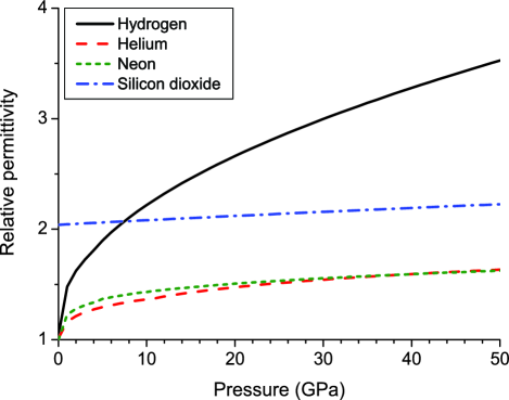
Figure 2: The pressure dependent permittivity of different materials. The permittivity of SiO₂ was calculated from the Vinet EOS and the Clausius-Mossotti relation. The other permittivites are based on literatureMediaProp .

Notice that there is no phase change in the SiO₂ curve. In nature SiO₂ is in a crystalline phase at zero pressure and will switch to the amorphous phase at about $90$ GPa. However, it has been reportedAmorfeSIO2kern that the fabrication method of the SiO₂ particles results in cores which are in the amorphous state also at zero pressure.

III Results for a nanoshell

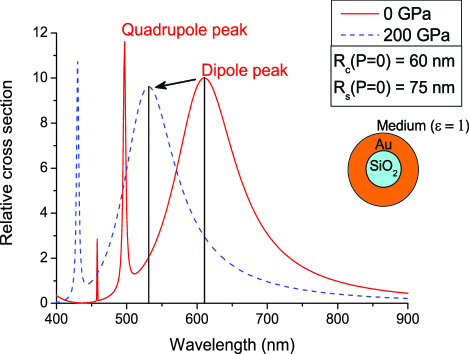
Figure 3: The relative cross section as a function of wavelength for different pressures for a nanoshell with parameters as mentioned in the figure. Notice the pressure-induced blueshift of the dipole peak from $611\operatorname{nm}$ at $0$ GPa to $531\operatorname{nm}$ at $200$ GPa as indicated by the two black lines.

Figure 3 shows the relative cross section of the considered nanoshell placed in vacuum as calculated with Mie theory. The relative cross section is the total optical cross section divided by $\pi R_{s}^{2}$, the area of the projection of the nanoshell on a plane perpendicular to the incoming radiation. From this figure one can clearly see a substantial blueshift when $200$ GPa pressure is applied. Another important observation concerns the width of the peak. This is important for increasing the precision in an experimental measurement since sharper peaks allow for a more accurate determination of the peak position. However, sharp resonance lines may elude experimental detection if they do not carry enough spectral weight. In Figure 3 one can see that the dipole peak (the rightmost peak) is a broad, clear and rather symmetric peak, while the quadrupole peak is much sharper and a good candidate for these kind of experiments. Numerically however it is easier to track the broad dipole peak, thus all results presented here will be with regard to the dipole peak. It is seen that although the quantitative results differ for all peaks, the qualitative results presented here hold true for all resonance peaks.

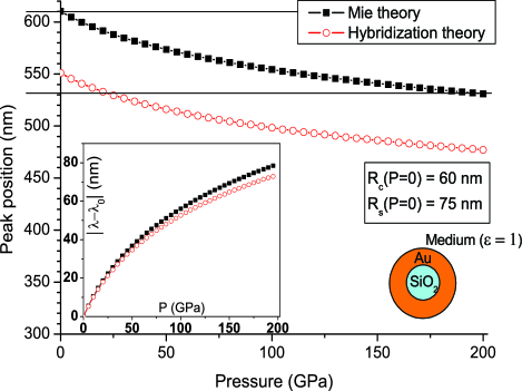
Figure 4: The position of the dipole resonance peak as a function of the pressure for a nanoshell with parameters as mentioned on the figure. The two horizontal black lines correspond to the two black lines on figure 3. The blueshift from $611\operatorname{nm}$ at $0$ GPa to $531\operatorname{nm}$ at $200$ GPa as predicted by Mie theory is clearly visible. The red circles were calculated with hybridization theory and also indicate a blueshift, but predict a different peak position. The inset shows the peak shift as a function of pressure compared to the original position at zero pressure.

In Figure 4 the position of the dipole resonance peak is shown as a function of pressure for a nanoshell in a medium with $\varepsilon=1$ constant. The black squares are calculated using Mie theory and a subsequent numerical determination of the peak maximum. The results from the hybridization theory are presented by the red circles. It is clear that the two theories do not agree on the exact position of the resonance peak for the considered nanoshell. This is due to the electrostatic limit used in the hybridization model which is only acceptable for nanoparticles much smaller than the wavelengths of the incident light (the limiting case for nanoshells much smaller than the wavelengths used in a DAC experiment, with sizes at the moment unachievable for fabrication, do agree). Still the hybridization model can prove to be useful because both theories agree well on the amount the peak shifts, as is shown in the inset of Figure 4. The two theories diverge from each other only at higher pressures. The results show that the nanoshell could be used to measure the pressure by determing the amount the resonance peak shifts. The inset is also an indication of the resolution that could be achieved. For this example nanoshell the dipole resonance peak shifts over $75\operatorname{nm}$ when $200$ GPa pressure is applied (for rubies this would be $51.1\operatorname{nm}$Ruby error ; Rubyto150GPa ).

To determine the usefulness of nanoshells as a pressure gauge, calibration would need to be done for every pressure medium separately. The nanoshell’s optical response depends on the dielectric function of the surrounding medium in which it is placed, and as such both the position of the resonance peaks and their pressure-induced shift will differ for different pressure media. The original data used for the calculation of the dielectric function are shown in table 2. In Figure 5

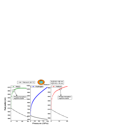
Figure 5: The position of the dipole peak as calculated with Mie theory for various pressure media: heliumMediaProp (red circles), hydrogenHydrogenSilvera (blue diamonds) and neonMediaProp (green triangles). In all figures the vacuum position is indicated in black for reference and the phase transition from liquid to solid is indicated. The plots only show the pressures for which experimental data is available. For completeness the original data are presented in table 2 together with the pressure range in which they are valid.

one can see the pressure dependency of the position of the dipole resonance peak for different pressure media: helium, hydrogen and neon. The behavior of the medium under pressure clearly has a large influence on the optical response of the nanoshell. For these media, the blueshift that occurs in vacuum has turned into a redshift as pressure is increased. From a certain pressure on, there will be almost no shift of the resonance peak, rendering the nanoshells ineffectual as pressure gauges in that region. Although it is possible to calculate the optical response of nanoshells for much higher pressures, the results are not presented here because they are based on extrapolation of data from a limited pressure region and as such are considered unreliable.

Table 2: The refractive index of materials used as pressure medium in a DAC as reported by references MediaProp and HydrogenSilvera . The last column presents the pressure range of the data on which these fits are based. The dielectric function $\varepsilon$ can be calculated by squaring the refractive index.

Material	Refractive index	$P$ range (GPa)
He (fluid)MediaProp	$n=0.8034+0.20256\left(1+P\right)^{0.12763}$	$0.08-11.5$
He (solid)MediaProp	$n=-0.1033+\left(1+P\right)^{0.052}$	$11.7-20.2$
H2HydrogenSilvera	$\begin{array}[c]{c}n=-0.687343+0.00407826P\\ +1.86605\left(0.29605+P\right)^{0.0646222}\end{array}$	$0-100$
Ne (fluid)MediaProp	$n=0.668+0.33\left(1+4.3P\right)^{0.076}$	$0.7-4.7$
Ne (solid)MediaProp	$n=0.9860+0.08597P^{0.1953}$	$5-27$

IV Results for a coated nanoshell

As was seen in the previous section, the simple nanoshell geometry is not ideal for high-pressure experiments. The peak shift is affected by the pressure medium so calibration will be necessary for each nanoshell and medium. A possible solution would be to shield the nanoparticle from the effects of the medium, therefore allowing the shift of the resonance peak to be influenced only by the compression of the nanoparticle. The absence of these problems when the nanoshell is placed in vacuum indicates that shielding the particle could indeed result in the desired effect.

Shielding the nanoparticle from the environments means creating a barrier between the golden shell and the dielectric medium. This barrier should also be a dielectric. If not, another set of surface plasmons polaritons would arise on the interface between the outer layer and the environment, counteracting the intent of the extra layer. In this article the extra coating is achieved by adding an extra SiO₂ layer to the model and extending Mie theory to three concentric spheres. Henceforth we shall indicate this type of ”nanomatryushka”nanomatr as ”coated nanoshell”. The main question to be answered is how thick this coating should be to effectively shield the nanoshell from the pressure effects on the dielectric function of the environment.

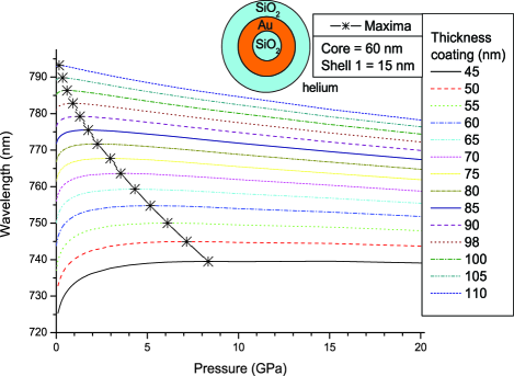
Figure 6: The dipole peak position as a function of pressure for the coated nanoshell with a $60\operatorname{nm}$ SiO₂ core, a $15\operatorname{nm}$ thick golden shell and for different thicknesses of the outer SiO₂ coating. For small coatings the redshift due to the medium is still clearly visible, while for thick coatings this effect seems to disappear. The black crosses indicate the pressure at which the wavelength peak position is maximal and where the redshift turns into a blueshift.

Figure 6 presents the dipole peak position for several coating thicknesses of the coated nanoshell as calculated by Mie theory. For reasons of comparison the core and the thickness of the golden shell are kept the same as for the nanoshell discussed before. Furthermore we have only studied the coated nanoshell in a helium environment since this is a commonly used quasi-hydrostatic pressure medium in DAC experiments. In neon the results will be almost the same because the dielectric functions of helium and neon are similar. For hydrogen the counteracting effect is not present, therefore the results with nanoshells are adequate and no further improvements are necessary.

In this article we do not compare the calculations for the coated nanoshell with calculations using the hybridization model. The expansion of the hybridization theory for multiple layered nanoshells is available in literatureHybri2 , but it is not considered here due to the expected deviations since the diameters of the coated nanoshell particles are $2$ or $3$ times larger than the nanoshell particles and thus the electrostatic approximation is certainly not valid.

It can be seen from Figure 6 that for thin coatings the redshift due to the effect of the medium is still visible. At a certain pressure the peak position will reach a maximum and from there on the peak will undergo a blueshift which is due to the compression of the nanoshell similar to the results in vacuum (Figure 4). This maximum is indicated by the black crosses and can be used as a measure for the pressure up to which the medium affects the optical response of the nanoparticle. It is clear that for thicker coatings the maximum shifts to lower pressures suggesting that the influence of the medium indeed diminishes and thus that the coating effectively shields the nanoparticle. Unfortunately the redshift never disappears completely meaning that the influence of the medium cannot be fully shielded by the dielectric layer. However, it is possible to position the maximum into a pressure region where it can do no harm for the pressure measurements.

Obviously, the thickness of the coating has to be adjusted to the needs of the experiments. A thicker coating will provide better shielding, but bigger particles take up more space and risk interacting with each other due to being in close proximity of one another. However, since the coated nanoshell is much larger than the nanoshell, the absolute cross section is larger, meaning that a smaller density is sufficient while still gaining the same response.

The derivative of the curves on Figure 6 give a direct indication of the sensitivity achievable with the coated nanoshell structures. On average the sensitivity for the coated nanoshell with a $110\operatorname{nm}$ thick coating (upper curve on Figure 6) is approximately $0.90$ $\operatorname{nm}/$GPa. The resolution for rubies in the same pressure regime ($0$ to $20$ GPa) is approximately $0.36$ $\operatorname{nm}/$GPaRuby error and for a nanoshell in vacuum as was shown in Figure 4 this would be $0.94$ $\operatorname{nm}/$GPa. From this we can conclude that the theory predicts a better resolution for nanoshells than for rubies in the pressure regime under consideration.

V Discussion and Conclusions

In this article we have carried out a theoretical analysis of nanoshells which can be designed so that they have absorption peaks in the IR-visible part of the optical spectrum due to scattering or absorption by localized surface plasmon polaritons. Calculations indicate that for nanoshells in vacuum these peaks have a substantial shift with pressure making them suitable as a pressure gauge for high-pressure research. A useful pressure gauge should have a calibration (peak wavelength vs pressure) independent of the pressurization medium. We found that for a simple nanoshell consisting of an SiO₂ core and a gold shell, the calibration differed with the pressurization medium; moreover it was double-valued and had a region of zero slope. The latter problem was resolved by coating the nanoshell with an SiO₂ cladding, resulting in a robust sensitive pressure gauge. The proposed nanoshell gauge has advantages in comparison with well-established pressure gauges: they will not easily blow out during loading of a DAC, they cannot easily be masked by fluorescence from the diamonds, they have large signal-to-noise ratio in comparison to fluorescence and Raman Scattering, and due to their small dimensions they will not be stressed by bridging between the diamonds at very high pressure when the gasket thins. All of these putative advantages must be confirmed by experiment.

A possible implementation of the coated nanoshell would be to distribute them inside the DAC cell together with the ruby on the diamond culet. For low pressures both gauges can be used and the coated nanoshell can be calibrated by using the extensive knowledge of the behavior of ruby under pressureRuby error . A possible challenge is the application of nanoshells to the surface of a diamond culet. Coated nanoshells can be acquired at high concentration $\left(2\sim 3\times 10^{9}/\operatorname{mm}^{3}\right)$ from Nanospectra Biosciences, Inc., in a liquid solution. A droplet can be placed on the culet and allowed to evaporate to produce a coverage bonded to the surface by van der Waals forces. Preliminary measurements show that to avoid clustering and segregation, it may prove useful to functionalize the diamond surface with a film of poly-4-vinylpyridine (pvp) which has dense sites that localize the nanoparticlesPVP . For high pressures the ruby measurement would be difficult or no longer be possible. The spectra of the coated nanoshells however will still be measurable since these measurements are based on absorption and transmission. In this way nanoshells could be easily used and effectively extend pressure measurements to ultra high pressures.

Appendix A Absorption and scattering of an electromagnetic wave by 3 concentric spheres.

The coated nanoshell was modeled using Mie theory for 3 concentric spheres. These spheres divide the space into 4 regions: the core of the nanoparticle, two shells and the medium in which the nanoparticle is immersed, respectively numbered $1$ through $4$ as shown in Figure 7.

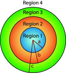
Figure 7: Schematic overview of the modeled system: region $1$ will be the SiO₂ core, region $2$ the golden shell, region $3$ the SiO₂ coating and region $4$ the pressure medium.

The radii of the three spheres are indicated with $a,b$ and $c$, from inner to outer. Using the notations of Bohren and Huffmanbohren the incoming plane wave can be expanded in vector spherical harmonics:

$$\vec{E}_{4,i} =\sum_{n=1}^{\infty}E_{n}\left(\vec{M}_{o1n}^{\left(1\right)}-i\vec{N}_{e1n}^{\left(1\right)}\right),$$ (10)

$$\vec{H}_{4,i} =\frac{-k_{4}}{\omega\mu_{4}}\sum_{n=1}^{\infty}E_{n}\left(\vec{M}_{e1n}^{\left(1\right)}+i\vec{N}_{o1n}^{\left(1\right)}\right),$$ (11)

with:

$$E_{n}=E_{0}i^{n}\frac{2n+1}{n\left(n+1\right)}.$$ (12)

The vector spherical harmonics can be written as:

$$\vec{M}_{e1n}^{\left(i\right)} =-z_{n}^{\left(i\right)}\left(kr\right)\pi_{n}\left(\cos\theta\right)\sin\varphi\vec{e}_{\theta}-z_{n}^{\left(i\right)}\left(kr\right)\tau_{n}\left(\cos\theta\right)\cos\varphi\vec{e}_{\varphi},$$ (13)

$$\vec{M}_{o1n}^{\left(i\right)} =z_{n}^{\left(i\right)}\left(kr\right)\pi_{n}\left(\cos\theta\right)\cos\varphi\vec{e}_{\theta}-z_{n}^{\left(i\right)}\left(kr\right)\tau_{n}\left(\cos\theta\right)\sin\varphi\vec{e}_{\varphi},$$ (14)

$$\vec{N}_{e1n}^{\left(i\right)} =\left(\frac{1}{kr}z_{n}^{\left(i\right)}\left(kr\right)n\left(n+1\right)\pi_{n}\left(\cos\theta\right)\sin\theta\cos\varphi\vec{e}_{r}\right.$$ (15)

$$\left.+dz_{n}^{\left(i\right)}\left(kr\right)\tau_{n}\left(\cos\theta\right)\cos\varphi\vec{e}_{\theta}-dz_{n}^{\left(i\right)}\left(kr\right)\pi_{n}\left(\cos\theta\right)\sin\varphi\vec{e}_{\varphi}\right),$$

$$\vec{N}_{o1n}^{\left(i\right)} =\left(\frac{1}{kr}z_{n}\left(kr\right)n\left(n+1\right)\pi_{n}\left(\cos\theta\right)\sin\theta\sin\varphi\vec{e}_{r}\right.$$ (16)

$$\left.+dz_{n}^{\left(i\right)}\left(kr\right)\tau_{n}\left(\cos\theta\right)\sin\varphi\vec{e}_{\theta}+dz_{n}^{\left(i\right)}\left(kr\right)\pi_{n}\left(\cos\theta\right)\cos\varphi\vec{e}_{\varphi}\right),$$

with the angle dependent functions (where $P_{n}^{m}\left(x\right)$ are the associated Legendre polynomials):

$$\pi_{n}\left(\cos\theta\right) =\frac{P_{n}^{1}\left(\cos\theta\right)}{\sin\theta},$$ (17)

$$\tau_{n}\left(\cos\theta\right) =\frac{dP_{n}^{1}\left(\cos\theta\right)}{d\theta},$$ (18)

and the radial dependent functions:

$$z_{n}^{1}\left(kr\right) =j_{n}\left(kr\right),$$ (19)

$$z_{n}^{2}\left(kr\right) =y_{n}\left(kr\right),$$ (20)

$$z_{n}^{3}\left(kr\right) =h_{n}^{\left(1\right)}\left(kr\right).$$ (21)

On the right hand side one can see the wel known spherical Bessel, Neumann and Hankel functions respectively.

In region $4$ there will also be a scattered wave which can be described by:

$$\vec{E}_{4,s} =\sum_{n=1}^{\infty}E_{n}\left(-a_{n}\vec{M}_{o1n}^{\left(3\right)}+ib_{n}\vec{N}_{e1n}^{\left(3\right)}\right),$$ (22)

$$\vec{H}_{4,s} =\frac{k_{4}}{\omega\mu_{4}}\sum_{n=1}^{\infty}E_{n}\left(b_{n}\vec{M}_{e1n}^{\left(3\right)}+ia_{n}\vec{N}_{o1n}^{\left(3\right)}\right),$$ (23)

where $a_{n}$ and $b_{n}$ are coefficients to be determined from the boundary conditions. The total electromagnetic wave in region $4$ is therefore given by the sum of the incoming and the scattered fields.

The electromagnetic fields in the other three regions are given by:

$$\left\{\begin{array}[c]{c}\vec{E}_{3}=\sum_{n=1}^{\infty}E_{n}\left(c_{n}^{\left(1\right)}\vec{M}_{o1n}^{\left(1\right)}+c_{n}^{\left(2\right)}\vec{M}_{o1n}^{\left(2\right)}-id_{n}^{\left(1\right)}\vec{N}_{e1n}^{\left(1\right)}-id_{n}^{\left(2\right)}\vec{N}_{e1n}^{\left(2\right)}\right)\\ \vec{H}_{3}=\frac{-k}{\omega\mu}\sum_{n=1}^{\infty}E_{n}\left(d_{n}^{\left(1\right)}\vec{M}_{e1n}^{\left(1\right)}+d_{n}^{\left(2\right)}\vec{M}_{e1n}^{\left(2\right)}+ic_{n}^{\left(1\right)}\vec{N}_{o1n}^{\left(1\right)}+ic_{n}^{\left(2\right)}\vec{N}_{o1n}^{\left(2\right)}\right)\end{array}\right.,$$ (26)

$$\left\{\begin{array}[c]{c}\vec{E}_{2}=\sum_{n=1}^{\infty}E_{n}\left(e_{n}^{\left(1\right)}\vec{M}_{o1n}^{\left(1\right)}+e_{n}^{\left(2\right)}\vec{M}_{o1n}^{\left(2\right)}-if_{n}^{\left(1\right)}\vec{N}_{e1n}^{\left(1\right)}-if_{n}^{\left(2\right)}\vec{N}_{e1n}^{\left(2\right)}\right)\\ \vec{H}_{2}=\frac{-k}{\omega\mu}\sum_{n=1}^{\infty}E_{n}\left(f_{n}^{\left(1\right)}\vec{M}_{e1n}^{\left(1\right)}+f_{n}^{\left(2\right)}\vec{M}_{e1n}^{\left(2\right)}+ie_{n}^{\left(1\right)}\vec{N}_{o1n}^{\left(1\right)}+ie_{n}^{\left(2\right)}\vec{N}_{o1n}^{\left(2\right)}\right)\end{array}\right.,$$ (29)

$$\left\{\begin{array}[c]{c}\vec{E}_{1}=\sum_{n=1}^{\infty}E_{n}\left(g_{n}\vec{M}_{o1n}^{\left(1\right)}-is_{n}\vec{N}_{e1n}^{\left(1\right)}\right)\\ \vec{H}_{1}=\frac{-k}{\omega\mu}\sum_{n=1}^{\infty}E_{n}\left(s_{n}\vec{M}_{e1n}^{\left(1\right)}+ig_{n}\vec{N}_{o1n}^{\left(1\right)}\right)\end{array}\right..$$ (32)

Using the boundary conditions:

$$\vec{E}_{j}\times\vec{e}_{r} =\vec{E}_{j+1}\times\vec{e}_{r},$$ (33)

$$\vec{H}_{j}\times\vec{e}_{r} =\vec{H}_{j+1}\times\vec{e}_{r}$$ (34)

at each interface, where $\vec{e}_{r}$ indicates the radial unit vector which is perpendicular to the boundary, we obtain a system of 12 coupled equations to be solved. This system of equations can be split in two sets of six equations that we write in matrix form $A_{i}\cdot x_{i}=b_{i}$ with for the first set of equations

$$A_{1}=\begin{bmatrix}0&0&0&j_{n}\left(k_{2}a\right)&y_{n}\left(k_{2}a\right)&-j_{n}\left(k_{1}a\right)\\ 0&0&0&dj_{n}\left(k_{2}a\right)&dy_{n}\left(k_{2}a\right)&-\frac{\mu_{2}k_{1}}{\mu_{1}k_{2}}dj_{n}\left(k_{1}a\right)\\ h_{n}^{\left(1\right)}\left(k_{4}c\right)&j_{n}\left(k_{3}c\right)&y_{n}\left(k_{3}c\right)&0&0&0\\ \frac{k_{4}\mu_{3}}{\mu_{4}k_{3}}dh_{n}^{\left(1\right)}\left(k_{4}c\right)&dj_{n}\left(k_{3}c\right)&dy_{n}\left(k_{3}c\right)&0&0&0\\ 0&j_{n}\left(k_{3}b\right)&y_{n}\left(k_{3}b\right)&-j_{n}\left(k_{2}b\right)&-y_{n}\left(k_{2}b\right)&0\\ 0&\frac{\mu_{2}k_{3}}{\mu_{3}k_{2}}dj_{n}\left(k_{3}b\right)&\frac{\mu_{2}k_{3}}{\mu_{3}k_{2}}dy_{n}\left(k_{3}b\right)&-dj_{n}\left(k_{2}b\right)&-dy_{n}\left(k_{2}b\right)&0\end{bmatrix},$$ (35)

and

$$b_{1}=\begin{bmatrix}0\\ 0\\ j_{n}\left(k_{4}c\right)\\ \frac{k_{4}\mu_{3}}{\mu_{4}k_{3}}dj_{n}\left(k_{4}c\right)\\ 0\\ 0\end{bmatrix},\qquad x_{1}=\begin{bmatrix}a_{n}\\ c_{n}^{\left(1\right)}\\ c_{n}^{\left(2\right)}\\ e_{n}^{\left(1\right)}\\ e_{n}^{\left(2\right)}\\ g_{n}\end{bmatrix}.$$ (36)

And for the second set of equations

$$A_{2}=\begin{bmatrix}0&0&0&dj_{n}\left(k_{2}a\right)&dy_{n}\left(k_{2}a\right)&-dj_{n}\left(k_{1}a\right)\\ 0&0&0&j_{n}\left(k_{2}a\right)&y_{n}\left(k_{2}a\right)&-\frac{\mu_{2}k_{1}}{\mu_{1}k_{2}}j_{n}\left(k_{1}a\right)\\ dh_{n}^{\left(1\right)}\left(k_{4}c\right)&dj_{n}\left(k_{3}c\right)&dy_{n}\left(k_{3}c\right)&0&0&0\\ \frac{k_{4}\mu_{3}}{\mu_{4}k_{3}}h_{n}^{\left(1\right)}\left(k_{4}c\right)&j_{n}\left(k_{3}c\right)&y_{n}\left(k_{3}c\right)&0&0&0\\ 0&dj_{n}\left(k_{3}b\right)&dy_{n}\left(k_{3}b\right)&-dj_{n}\left(k_{2}b\right)&-dy_{n}\left(k_{2}b\right)&0\\ 0&\frac{\mu_{2}k_{3}}{\mu_{3}k_{2}}j_{n}\left(k_{3}b\right)&\frac{\mu_{2}k_{3}}{\mu_{3}k_{2}}y_{n}\left(k_{3}b\right)&-j_{n}\left(k_{2}b\right)&-y_{n}\left(k_{2}b\right)&0\end{bmatrix},$$ (37)

$$b_{2}=\begin{bmatrix}0\\ 0\\ dj_{n}\left(k_{4}c\right)\\ \frac{k_{4}\mu_{3}}{\mu_{4}k_{3}}j_{n}\left(k_{4}c\right)\\ 0\\ 0\end{bmatrix},\qquad x_{2}=\begin{bmatrix}b_{n}\\ d_{n}^{\left(1\right)}\\ d_{n}^{\left(2\right)}\\ f_{n}^{\left(1\right)}\\ f_{n}^{\left(2\right)}\\ s_{n}\end{bmatrix}.$$ (38)

These equations are solved by matrix inversion. Hence the total solution in every region is known. The optical cross section can now be calculated by:

$$Q_{scatt} =\frac{2\pi}{k_{4}^{2}}\sum_{n=1}^{\infty}\left(2n+1\right)\left(\left|a_{n}\right|^{2}+\left|b_{n}\right|^{2}\right),$$ (39)

$$Q_{abs} =\frac{2\pi}{k_{4}^{2}}\sum_{n=1}^{\infty}\left(2n+1\right)\left(\left|a_{n}\right|^{2}+\left|b_{n}\right|^{2}-\operatorname{Re}\left(a_{n}+b_{n}\right)\right),$$ (40)

$$Q_{tot} =\frac{2\pi}{k_{4}^{2}}\sum_{n=1}^{\infty}\left(2n+1\right)\operatorname{Re}\left(a_{n}+b_{n}\right),$$ (41)

where $a_{n}$ and $b_{n}$ are the coefficients of the scattered wave as introduced in equations $\left(\ref{eq scatt E}\right)$ and $\left(\ref{eq scatt H}\right)$. The wave vector $k$ can be calculated from

$$k_{i}^{2}=\omega^{2}\varepsilon_{i}\mu_{i}$$ (42)

with $\varepsilon_{i}$ de permittivity and $\mu_{i}$ the permeability of the $i^{the}$ region.

References

- (1) L.R. Hirsch, A.M. Gobin, A.R. Lowery, F. Tam, R.A. Drezek, N.J. Halas and J.L. West, Annals of biomedical engineering 34, 15 .
- (2) J. Yang, J. Lee, J. Kang, S.J. Oh, H.-J. Ko, J.-H. Son, K. Lee, J-S.. Suh, Y.-M. Huh and S. Haam, Adv. Matter 21, 1 .
- (3) M.L. Brongersma, Nature materials 2, 296 .
- (4) J.B. Jackson, S.L. Westcott, L.R. Hirsch, J.L. West and N.J. Halas, Appl. Phys. Letters 82, 257 .
- (5) S. Lal, S. Link and N.J. Halas, Nature photonics 1, 641 .
- (6) A. Jayaraman, Rev. Mod. Phys 55, 1 .
- (7) H.K. Mao, J. Xu and P.M. Bell, Journal of geophysical research 91, 4673 .
- (8) G.J. Piermarini, S.J. Block, J.D. Barnett and R.A. Forman, J. Appl. Phys., 46, 2774 .
- (9) I.F. Silvera, A.D. Chijioke, W.J. Nellis, A. Soldatov and J. Tempere, Phys. Stat. Sol (b) 244, 460 .
- (10) A. Chijioke, W.J. Nellis, A. Soldatov and I.F. Silvera, J. Appl. Phys. 98, 114905,
- (11) J.H. Eggert, K.A. Goetel and I.F. Silvera, Appl. Phys. Letters 53, 2489
- (12) N.H. Chen and I.F. Silvera, Rev. Sci. Instrum. 67, 4275
- (13) B.J. Baer, M.E., Chang and W.J. Evans, J. Appl. Phys. 104, 034504 .
- (14) N. Dubrovinskaia, L. Dubrovinsky, R. Caracas and M. Hanfland, Appl. Phys. Letters 97, 251903
- (15) E. Prodan, C. Radloff, N.J. Halas and P. Nordlander, Science 302, 419 .
- (16) J.A. Stratton, Electromagnetic theory (McGraw-Hill book company, New York and London ), p.563-573.
- (17) C. Kittel, Introduction to solid state physics, fifth edition (John Wiley & Sons, USA ), p.410.
- (18) C. Radloff and N.J. Halas, Nano Letters 4, 1323 .
- (19) E. Prodan and P. Nordlander, J. Chem. Phys. 120, 5444 .
- (20) A.L. Aden and M. Kerker, J. Appl. Phys. 22, 1242 .
- (21) P. Vinet, J. Ferrante, J.H. Rose and J.R. Smith, Journal of geophysical research 92, 9319 .
- (22) K.P. Driver, R.E. Cohen, Z. Wu, B. Militzer, P.L. Rios, M.D. Towler, R.J. Needs and J.W. Wilkins, Proc. Natl. Acad. Sci. USA 107, 9519 .
- (23) C.E. Rayford II, G. Schatz and K. Shuford, Nanoscape 2, 27 .
- (24) M. Yokoo, N. Kawai, K.G. Nakamura, K-I Kondo, Y. Tange and T. Tsuchiya, Phys. Rev. B 80, 104114 .
- (25) I.N. Shklyarefskii and P.L. Pakhmov, USSR optika i Spektroskopiya 34, 163 also at http://www.mit.edu/~6.777/matprops/gold.htm.
- (26) S. Kalele, S.W. Gosavi, J. Urban and S.K. Kulkarni, Current science 19, 1038 .
- (27) A. Dewaele, J.H. Egert, P. Loubeyre and R. Le Toullec, Phys. Rev. B 67, 094112 .
- (28) W.J. Evans and I. F. Silvera, Phys. Rev. B 57, 14105 .
- (29) C.F. Bohren and D.R. Huffman, Absorption and scattering of light by small particles (Wiley-VCH, Germany ), p.82-104.
- (30) S. Malynych, I. Luzinov and G. Chymanov, J. Phys. Chem. B 106, 1280 .