Radiative corrections to anti-neutrino proton scattering at low energies

U. Raha, F. Myhrer and K.Kubodera
Department of Physics and Astronomy, University of South Carolina, Columbia, SC 29208

For the low-energy anti-neutrino reaction, $\bar{\nu}_{e}+p\to e^{+}+n$, which is of great current interest in connection with on-going high-precision neutrino-oscillation experiments, we calculate the differential cross section in a model-independent effective field theory (EFT), taking into account radiative corrections of order $\alpha$. In EFT, the short-distance radiative corrections are subsumed into well-defined low-energy constants the values of which can in principle be determined from the available neutron beta-decay data. In our low-energy EFT, the order-$\alpha$ radiative corrections are considered to be of the same order as the nucleon recoil corrections, which include the “weak magnetism” contribution. These recoil corrections have been evaluated as well. We emphasize that EFT allows for a systematic evaluation of higher order corrections, providing estimates of theoretical uncertainties in our results.

1 Introduction

Low-energy anti-neutrinos from nuclear reactors are well suited to determine the neutrino mixing angle $\theta_{13}$, which is important for the search of CP violation in the leptonic sector; see, e.g., Refs. [1, 2]. The Double-Chooz [3], Daya Bay [4], and RENO Collaborations [5] are aiming to measure $\theta_{13}$ with very high precision with the use of $\bar{\nu}_{e}$’s produced in nuclear reactors. The present upper bound to this quantity reported by the Chooz [3] and MINOS [6] Collaborations is: $\theta_{13}<11.4^{\circ}$.

The Double-Chooz, Daya Bay and RENO experiments monitor the inverse beta-decay reaction on a hydrogen target

$$\bar{\nu}_{e}+p\to e^{+}+n$$ (1)

for a known anti-neutrino energy flux. The positron yield is measured as a function of the positron energy. An accurate extraction of the mixing angle $\theta_{13}$ from an analysis of the measured positron yield requires a precise knowledge of the radiative corrections (RCs). In earlier papers [7, 8, 9], the relevant RCs were evaluated in the theoretical framework developed by Sirlin and Marciano [10, 11]. In this framework, to be referred to as the S-M approach, the RCs of order $\alpha$ are decomposed into so-called outer and inner corrections. The outer correction is a universal function of the lepton energy and is independent of the details of hadron physics, whereas the inner correction is influenced by short-distance physics and the hadron structure. The inner corrections coming from $\gamma$ and weak-boson loop diagrams are divided into high-momentum and low-momentum parts. The former is evaluated in the current-quark picture, while the latter is computed with the use of the phenomenological electroweak-interaction form factors of the nucleon. Although the estimates of inner corrections in the S-M formalism are considered to be reliable to the level of accuracy quoted in the literature, the possibility that these estimates may involve some degree of model dependence is not totally excluded.

We present here a calculation of the RCs to order $\alpha$ based on effective field theory (EFT). We use heavy-baryon chiral perturbation theory (HB$\chi$PT), which is an effective low-energy theory of QCD, see e.g. Ref [12]. In HB$\chi$PT the short distance hadronic and electroweak processes are subsumed into a well-defined set of low-energy constants (LECs). In other words, these LECs systematically parameterize the inner corrections of the S-M approach. Therefore, insofar as there are enough sources of information to determine the values of these LECs, HB$\chi$PT leads to model-independent results with systematic estimates of higher-order corrections. The use of HB$\chi$PT to calculate electroweak transition amplitudes for the nucleon and few-nucleon systems were pioneered in Refs. [13, 14, 15], and subsequently there have been many important developments. In Ref. [16], we presented the first ever EFT-based calculation of RCs for the neutron $\beta$-decay process, $n\to p+e^{-}+\!\bar{\nu}_{e}$. Because in HB$\chi$PT the nucleons are treated as point-like, it is expected on general grounds that the order-$\alpha$ RCs are common between neutron $\beta$-decay and inverse $\beta$-decay. Meanwhile, it should be mentioned that, in the counting scheme adopted here and in Ref.[16], the order-$\alpha$ RCs are of the same order as the $m_{\mbox{\tiny N}}^{-1}$ nucleon-recoil corrections including the “weak magnetism” contributions, and hence a consistent EFT calculation should include these recoil corrections simultaneously. We present here such an EFT calculation, taking advantage of the fact that the $m_{\mbox{\tiny N}}^{-1}$-expansion is a natural part of our counting scheme and thus dictates how to incorporate recoil corrections order by order (see later in the text).

Since exactly the same LECs are involved in the EFT calculations of inverse $\beta$-decay and neutron $\beta$-decay, we can in principle use the existing neutron $\beta$-decay data to determine those LECs and make a model-independent estimation of RCs for the inverse $\beta$-decay, provided that the $m_{\mbox{\tiny N}}^{-1}$ recoil corrections are properly taken into account. In this connection, we note that an attempt has been made in the literature [7, 19] to directly relate the neutron decay rate with the inverse $\beta$-decay cross section, assuming that the order-$\alpha$ corrections (RCs and recoil corrections combined) are common between these processes. As mentioned, this assumption is justified as far as the genuine RCs of order $\alpha$ is concerned. However, as described later in the text, our calculation shows differences between the $m_{\mbox{\tiny N}}^{-1}$ corrections for inverse $\beta$-decay, Eq. (1), and those for neutron $\beta$-decay. We therefore caution against writing the cross section for the reaction in Eq. (1) in terms of the neutron mean life, $\tau_{n}$, as advocated in Refs. [7, 19].

This paper is organized as follows. In section 2 we explain a theoretical framework to be used and present the results for the order-$\alpha$ RCs. In section 3 we consider the recoil corrections and compare our results with an earlier work[19]. Section 4 gives a summary of our calculations and conclusions. The appendix describes some technical details concerning the HB$\chi$PT treatment of the infrared singularity.

2 The QED corrections

We use here essentially the same theoretical framework as in Ref. [16], in which we calculated RCs for neutron $\beta$-decay. We therefore give only a brief recapitulation of our formalism, relegating details to Ref. [16].

Our calculation is based on the $\bar{Q}/\Lambda_{\chi}$-expansion scheme, where $\bar{Q}$ $\sim$ $E_{\nu}\!-\!\Delta_{N}\!-\!m_{e}$ ($\Delta_{N}=m_{n}-m_{p}$) represents a typical four-momentum transfer for incident low-energy reactor anti-neutrinos ($E_{\nu}\leq 10$ MeV), and $\Lambda_{\chi}\simeq 4\pi f_{\pi}\approx 1$ GeV ($f_{\pi}=92.4$ MeV is the pion-decay constant) is the chiral scale. It is to be noted that the expansion parameter in our scheme is very small and that, as explained in more detail below, the lowest order recoil corrections $\sim\bar{Q}/m_{\mbox{\tiny N}}$ are of the same order as the lowest order radiative corrections; viz., $\bar{Q}/m_{\mbox{\tiny N}}\sim\alpha/(2\pi)\sim\bar{Q}/\Lambda_{\chi}\sim 10^{-3}$, where $m_{\mbox{\tiny N}}=(m_{p}\!+\!m_{n})/2$.

The leading order (LO) transition matrix element for the inverse $\beta$-decay, Eq.(1), is evaluated ignoring nucleon recoil and radiative corrections. The next-to-leading order (NLO) corrections in our counting scheme are the recoil corrections ($\sim Q/m_{\mbox{\tiny N}}$) and the radiative corrections ($\sim\alpha/(2\pi)$). The recoil corrections, which include the “weak magnetism” term, will be specified in Eq.(LABEL:eq:Lnnee) below. For the sake of the transparency of presentation, we shall in this paper separate these corrections from the $m_{\mbox{\tiny N}}^{-1}$ (kinematic) corrections to the phase-space.

The effective lagrangian relevant to our calculation includes the relativistic leptonic weak interaction current and the LO and NLO heavy-baryon lagrangian

$${\cal L}_{eff} = {\cal L}_{QED}+{\cal L}_{NN}+{\cal L}_{NN\psi\psi}\;,$$ (2)

where

$${\cal L}_{QED}\!\! = \!-\frac{1}{4}F^{\mu\nu}\!F_{\mu\nu}-\frac{1}{2\xi_{A}}(\partial\!\cdot\!A)^{2}+\left(\!1\!+\!\frac{\alpha}{4\pi}e_{1}\!\right)\!\bar{\psi}_{e}(i\gamma\!\cdot\!D)\psi_{e}+m_{e}\bar{\psi}_{e}\psi_{e}+\bar{\psi}_{\nu}i\gamma\!\cdot\!\partial\psi_{\nu},$$ (3)

$${\cal L}_{NN}\!\! = \!\bar{N}\left[1+\frac{\alpha}{8\pi}e_{2}(1+\tau_{3})\right](iv\cdot D)N\;,$$ (4)

$${\cal L}_{NN\psi\psi}\! = \!\!\!\!-\!\left(\frac{G_{F}V_{ud}}{\sqrt{2}}\right)\!\left[\bar{\psi}_{e}\gamma_{\mu}(1-\gamma_{5})\psi_{\nu}\right]\!\left\{\bar{N}\tau^{+}\!\left[\left(1\!+\!\frac{\alpha}{4\pi}e_{\mbox{\tiny V}}\right)v^{\mu}-2g_{A}\!\left(1\!+\!\frac{\alpha}{4\pi}e_{\mbox{\tiny A}}\right)S^{\mu}\right]\!N\right.$$

$$+ \!\!\!\left.\!\!\frac{1}{2m_{N}}\bar{N}\tau^{+}\!\!\left[i(v^{\mu}v^{\nu}\!\!-\!g^{\mu\nu})(\stackrel{{\scriptstyle\leftarrow}}{{\partial}}\!-\!\stackrel{{\scriptstyle\rightarrow}}{{\partial}})_{\nu}\!-\!2i\mu_{\mbox{\tiny V}}\!\left[S^{\mu}\!,S\!\cdot\!(\stackrel{{\scriptstyle\leftarrow}}{{\partial}}\!+\!\stackrel{{\scriptstyle\rightarrow}}{{\partial}})\right]\!-\!2ig_{\mbox{\tiny A}}v^{\mu}S\!\cdot\!(\stackrel{{\scriptstyle\leftarrow}}{{\partial}}\!-\!\stackrel{{\scriptstyle\rightarrow}}{{\partial}})\right]\!N\right\}.$$

${\cal L}_{QED}$ in Eq.(3) is the usual QED lagrangian, where $F_{\mu\nu}\!=\!\partial_{\mu}A_{\nu}\!-\!\partial_{\nu}A_{\mu}$, and $D_{\mu}=\partial_{\mu}\!+\!ieA_{\mu}$ is the covariant derivative; for the gauge parameter $\xi_{A}$, we use here $\xi_{A}=1$ (Feynman gauge). ${\cal L}_{NN}$ is the heavy-nucleon lagrangian including the photon-nucleon interaction, and ${\cal L}_{NN\psi\psi}$ is the low-energy LO and NLO current-current weak interaction. We give in Eq.(LABEL:eq:Lnnee) the explicit forms of NLO nucleon-recoil terms dictated by HB$\chi$PT. In the above, $g_{A}=1.267$ is the axial coupling constant, while $v_{\mu}$ is the nucleon velocity vector, and $S^{\mu}$ is the nucleon spin; they satisfy $v\cdot S=0$. We choose here $v^{\mu}=(1,\vec{0})$ and $S^{\mu}=(0,\vec{\sigma}/2)$. In the NLO part of the lagrangian the nucleon isovector magnetic moment $\mu_{\mbox{\tiny V}}=\mu_{p}\!-\!\mu_{n}=4.706$. The low-energy constants (LECs), $e_{1}$, $e_{2}$, $e_{\mbox{\tiny V}}$ and $e_{\mbox{\tiny A}}$, are counter-terms which regulate the ultraviolet (UV) divergences of the virtual photon-loop diagrams. These LECs incorporate the short-range radiative physics that is not probed in a low-energy process. The LECs, $e_{1}$ and $e_{2}$, are related to the wave-function renormalization factors of the positron and proton, respectively. The LECs, $e_{\mbox{\tiny V}}$ and $e_{\mbox{\tiny A}}$, are related to the Fermi and Gamow-Teller amplitudes. The Fermi coupling constant, $G_{F}=1.166\times 10^{-5}$ GeV^-2, is determined from muon decay, and the CKM matrix element, $|V_{ud}|=0.97418\pm 0.00027$, is given by the PDG [20].

For later convenience, we rearrange the LECs in Eq.(LABEL:eq:Lnnee) by rewriting the hadronic part in the first line in Eq.(LABEL:eq:Lnnee) as

$$\bar{N}\tau^{+}\!\left[v^{\mu}\!-\!2\tilde{g}_{\mbox{\tiny A}}S^{\mu}\right]\!N+\left(\frac{\alpha}{4\pi}\right)\!e_{\mbox{\tiny V}}\bar{N}\tau^{+}\!\left[v^{\mu}\!-\!2\tilde{g}_{\mbox{\tiny A}}S^{\mu}\right]\!N+{\cal O}(\alpha^{2})\;,$$

where we have introduced the redefined axial coupling constant, $\tilde{g}_{\mbox{\tiny A}}=g_{\mbox{\tiny A}}[1\!+\!\frac{\alpha}{4\pi}(e_{\mbox{\tiny A}}\!-\!e_{\mbox{\tiny V}})]$. As in the neutron $\beta$-decay case [16], to the order of our concern, $g_{\mbox{\tiny A}}$ can always be replaced by $\tilde{g}_{\mbox{\tiny A}}$. This also applies to the NLO recoil contributions since the $m_{\mbox{\tiny N}}^{-1}$ recoil corrections are of the same order as order-$\alpha$ corrections in the adopted counting scheme. The order-$\alpha$ radiative corrections to the nucleon magnetic moments are for the same reason of higher order in our scheme and hence neglected in this work.

In this paper we derive a model-independent expression for the lowest order radiative and recoil corrections to the reaction, $\bar{\nu}_{e}(p_{\nu})+p(p_{p})\to e^{+}(p_{e})+n(p_{n})$, where the four-momentum of each particle is indicated in the parentheses. We shall concentrate on an experimental setup in which none of the particle spins are monitored by the detector. There is one subtle aspect of the above reaction which deserves some discussion. In experiments, the final state positron will always be accompanied by (often undetected) soft bremsstrahlung photons. If the bremsstrahlung photon energy, $E_{\gamma}$ is less than the detector resolution, $\Delta$, the energy recorded by the detector is the sum of the actual outgoing positron energy, $E_{e}$, and the bremsstrahlung photon energy, $E_{\gamma}$; i.e., $E=E_{e}+E_{\gamma}$ is what is measured as the “detected positron” energy, with the corresponding “detected positron” momentum being $|\mbox{\boldmath$p$}|=\sqrt{E^{2}-m^{2}_{e}}$. The two processes we evaluate are $\bar{\nu}_{e}+p\to e^{+}+n$ and $\bar{\nu}_{e}+p\to e^{+}+\gamma+n$. Due to the finite detector resolution the second bremsstrahlung process is not observed; it only contributes to the RCs of the first process, i.e., the soft bremsstrahlung photons are an integral part of the “detected positron”. Thus, the first process has become, $\bar{\nu}_{e}(p_{\nu})+p(p_{p})\to e^{+}(p)+n(p_{n})$, where the positron momentum $p_{e}$ has been replaced by $p$ in order to indicate that the soft bremsstrahlung process has been incorporated into this “effective” reaction. The cross section for this “effective” reaction is given in terms of the effective invariant amplitude ${\cal M}$:

$${\rm d}\sigma\!\!\! = \!\!\!\frac{1}{4m_{p}E_{\nu}}\int\frac{{\rm d}^{3}\mbox{\boldmath$p$}}{(2\pi)^{3}2E}\frac{{\rm d}^{3}\mbox{\boldmath$p$}_{n}}{(2\pi)^{3}2E_{n}}(2\pi)^{4}\delta^{(4)}(p_{\nu}\!+\!p_{p}\!-\!p\!-\!p_{n})\,\frac{1}{2}\sum_{\rm spins}|{\cal M}|^{2}$$ (6)

$$= \!\!\left(\frac{G_{F}V_{ud}}{\sqrt{2}}\right)^{2}\!\!f(E)\left[(1\!+\!3g_{A}^{2})\,{\cal G}_{1}(\beta)+(1\!-\!g_{A}^{2})\,{\cal G}_{2}(\beta)\beta\cos\theta_{e}\right]{\rm d}(\cos\theta_{e})\,,$$

where $\beta=|\mbox{\boldmath$p$}|/E=\sqrt{E^{2}-m^{2}_{e}}/E$ is the velocity of the outgoing “detected positron” for a given incident (anti-)neutrino beam energy, $E_{\nu}$ and detector reading, $E$; $\cos(\theta_{e})=\hat{\mbox{\boldmath$p$}}_{\nu}\!\cdot\hat{\mbox{\boldmath$p$}}$, and $f(E)$ is the phase-space factor to be discussed later in the text (see, Eq. (17)). The two velocity-dependent functions, ${\cal G}_{i}(\beta)$ ($i=1,\ 2$), are written up to NLO as

$${\cal G}_{i}(\beta)\! = \!\!1+\frac{\alpha}{2\pi}\,{\cal G}_{i}^{rad}(\beta)+\frac{1}{m_{\mbox{\tiny N}}}\,{\cal G}_{i}^{recoil}(\beta)\;,$$ (7)

Here ${\cal G}_{i}^{rad}(\beta)$ (see, Eqs. (10) and (11)) represent the lowest-order radiative corrections, and ${\cal G}_{i}^{recoil}(\beta)$ (see, Eq. (18)), which will be evaluated in the next section, represent the recoil corrections arising from the lagrangian in Eq.(LABEL:eq:Lnnee). The calculation of the function ${\cal G}_{i}^{rad}(\beta)$ is described next.

For the analysis of the radiative corrections, we explicitly distinguish between the outgoing positron and the bremsstrahlung photon. There are two distinct categories of radiative corrections, the bremsstrahlung and the virtual photon loop corrections. The corresponding Feynman diagrams are shown in Fig. 1. Since ${\cal O}(\alpha)$ and ${\cal O}(m_{N}^{-1})$ are of the same order in our counting scheme, the invariant matrix element, ${\cal M}_{br}$ for bremsstrahlung is evaluated assuming $E_{n}=m_{n}$. The differential cross section for the radiative process, $\bar{\nu}_{e}(p_{\nu})\!+\!p(p_{p})\!\to\!e^{+}(\tilde{p}_{e})\!+\!n(p_{n})\!+\!\gamma(\tilde{k})$, is given by

$${\rm d}\sigma_{br}(\bar{\nu}_{e}p\to e^{+}n\gamma) = \frac{1}{8m_{p}m_{n}E_{\nu}}\int\frac{{\rm d}^{3}\tilde{\mbox{\boldmath$p$}}_{e}}{(2\pi)^{3}2\tilde{E}_{e}}\frac{{\rm d}^{3}\tilde{\mbox{\boldmath$k$}}}{(2\pi)^{3}2\tilde{E}_{\gamma}}$$ (8)

$$\times (2\pi)\delta(E_{\nu}-\Delta_{N}-\tilde{E}_{\gamma}-\tilde{E}_{e})\frac{1}{2}\sum_{spins}|{\cal M}_{br}|^{2}\;,$$

where $\tilde{E}=\tilde{E}_{e}+\tilde{E}_{\gamma}=E_{\nu}-\Delta_{N}$ is the maximum energy of the “detected positron” in the static nucleon approximation, i.e., $m_{e}\leq E\leq\tilde{E}$. The bremsstrahlung matrix element squared with the static neutron is

$$\frac{1}{2}\sum|{\cal M}_{br}|^{2} = \left(\frac{eG_{F}V_{ud}}{\sqrt{2}}\right)^{2}\left(\frac{32m_{n}m_{p}\tilde{E}_{e}E_{\nu}}{\tilde{E}_{\gamma}(\tilde{p}_{e}\cdot\tilde{k})}\right)$$ (9)

$$\times \!\!\!\!\left\{-\left[\frac{(1+3g_{A}^{2})(\tilde{p}_{e}\cdot\tilde{k})}{\tilde{E}_{\gamma}}\right]\left[1+\left(\frac{1-g_{A}^{2}}{1+3g_{A}^{2}}\right)\frac{\tilde{\mbox{\boldmath$p$}}_{e}\cdot\mbox{\boldmath$p$}_{\nu}}{\tilde{E}_{e}E_{\nu}}\right]\right.$$

$$+ \!\!\!(1\!+\!3g_{A}^{2})\Big{[}\frac{2\tilde{E}_{e}^{2}+\tilde{E}_{e}\tilde{E}_{\gamma}+\tilde{\mbox{\boldmath$p$}}_{e}\cdot\tilde{\mbox{\boldmath$k$}}+\tilde{E}_{\gamma}^{2}}{\tilde{E}_{e}}-\ \frac{m_{e}^{2}\tilde{E}_{\gamma}(\tilde{E}_{e}+\tilde{E}_{\gamma})}{\tilde{E}_{e}(\tilde{p}_{e}\cdot\tilde{k})}\Big{]}$$

$$+ \!\!(1-g_{A}^{2})\Big{[}(\tilde{\mbox{\boldmath$p$}}_{e}\cdot\mbox{\boldmath$p$}_{\nu})\left(\frac{2\tilde{E}_{e}+\tilde{E}_{\gamma}}{\tilde{E}_{e}E_{\nu}}-\frac{m_{e}^{2}\tilde{E}_{\gamma}}{\tilde{E}_{e}E_{\nu}(\tilde{p}_{e}\cdot\tilde{k})}\right)\Big{]}$$

$$+ \left.\!\!(1-g_{A}^{2})\Big{[}(\tilde{\mbox{\boldmath$k$}}\cdot\mbox{\boldmath$p$}_{\nu})\left(\frac{\tilde{E}_{e}+\tilde{E}_{\gamma}}{\tilde{E}_{e}E_{\nu}}-\frac{m_{e}^{2}\tilde{E}_{\gamma}}{\tilde{E}_{e}E_{\nu}(\tilde{p}_{e}\cdot\tilde{k})}\right)\Big{]}\right\}\;.$$

We note that the above expression for $\sum|{\cal M}_{br}|^{2}$ is identical to that for neutron $\beta$-decay derived in Ref. [16]. We also remark that Eq.(9) was derived earlier by Fukugita and Kubota [9], who used the S-M approach [10, 11] and a finite photon mass in order to regulate the infrared (IR) singularity. In the integration over the bremsstrahlung photon energy in Eq.(8) the maximum photon energy occurs when $\tilde{E}_{e}\!=\!m_{e}$, i.e., $\tilde{E}^{max}_{\gamma}=\tilde{E}-m_{e}$. In this context, the same question again arises as to whether or not the experiment can distinguish between the two final states, $n+e^{+}+\gamma$ and $n+e^{+}$. If the detector resolution in the experimental setup is such that one can detect photons with an energy $\tilde{E}_{\gamma}$ in the interval $\Delta\leq\tilde{E}_{\gamma}\leq\tilde{E}_{\gamma}^{max}$, we should integrate the bremsstrahlung photon energy $\tilde{E}_{\gamma}=|\tilde{\mbox{\boldmath$k$}}|$ from 0 to $\Delta$ in Eq. (8). However, if the experiment is unable to distinguish these two final states, we should integrate from 0 to $\tilde{E}_{\gamma}^{max}$. In order to compare with earlier works, we concentrate here on the latter case. The integral over the radiative photon spectrum invariably gives rise to an IR singularity. We use dimensional regularization to deal with the IR singularity; some details regarding the bremsstrahlung integral are presented in the appendix. As is well known, the IR singularity appearing in Eq.(8) is cancelled by the contributions from virtual photon-loop diagrams in accordance with Bloch and Nordsieck [17], see also [18]. The evaluation of the loop diagrams in dimensional regularization can be found in the literature, see, e.g., Ref. [16]. It is notable that, apart from the so-called “Coulomb factor” $\pi^{2}/\beta$, which arises in, e.g. neutron $\beta$-decay from a photon-loop diagram, the matrix element given by these virtual photon loops is identical to the one in neutron $\beta$-decay.

The UV-divergencies originating from the photon loop diagrams are regulated by the LECs in the lagrangian. These LECs are renormalized by the usual effective field theoretical method based on dimensional regularization of the loop integrals, see e.g., Refs. [12, 22]. The finite LECs renormalized at the scale $\mu$ are

$$e_{V,A}^{R}(\mu^{2})=e_{V,A}-\frac{1}{2}(e_{1}+e_{2})+\frac{3}{2}\left[\frac{2}{d-4}-\gamma_{E}+{\rm ln}(4\pi)+1\right]+\frac{3}{2}\,{\rm ln}\left(\frac{\mu^{2}}{m_{N}^{2}}\right)\;.$$

The LEC, $e_{\mbox{\tiny V}}^{R}(\mu^{2})$, which was introduced by Ando et al. [16] in the evaluation of the RC for neutron $\beta$-decay, subsumes short distance physics not probed at low energies and depends on the regularization scale $\mu$.

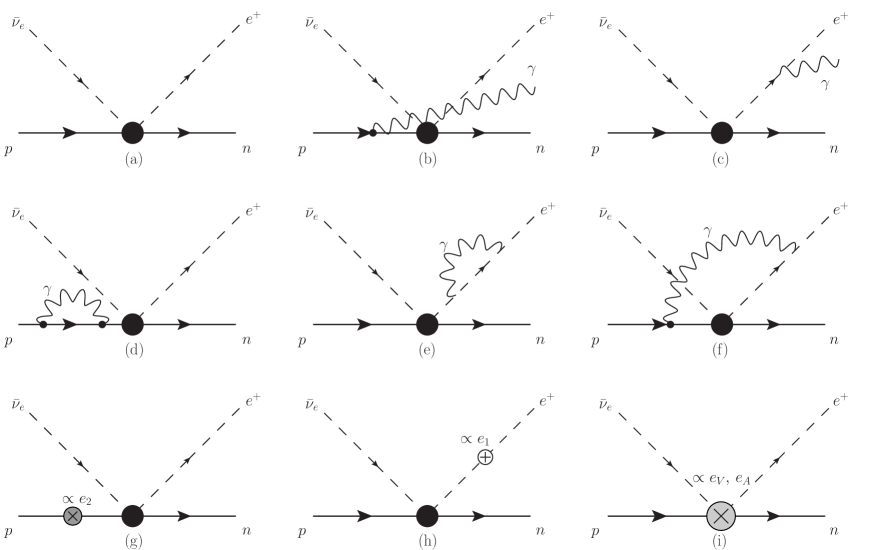
Figure 1: Feynman diagrams contributing to the cross section which includes ${\mathcal{O}}(\alpha)$ QED corrections: (a) — leading order (LO) Born amplitude; (b) and (c) — bremsstrahlung amplitudes; (d), (e) and (f) — virtual photon-loop diagrams; (g) and (h) — counter-term amplitudes involving the LECs $e_{1}$ and $e_{2}$, respectively; (i) — counter-term amplitudes involving both of the LECs, $e_{\mbox{\tiny V}}$ and $e_{\mbox{\tiny A}}$. The $m_{\mbox{\tiny N}}^{-1}$ correction is represented by diagram (a) but with the use of the vertex that arises from the $m_{\mbox{\tiny N}}^{-1}$ (NLO) part of the lagrangian in Eq.(LABEL:eq:Lnnee). To the order of our concern we do not consider diagrams in which a photon couples to the nucleon magnetic moments since this is ${\cal O}(\alpha/m_{N})$ or NNLO.

Combining the bremsstrahlung and virtual photon-loops contributions calculated to order $\alpha$, and noting that $\tilde{\beta}=\sqrt{\tilde{E}^{2}-m^{2}_{e}}/\tilde{E}=\beta+\mathcal{O}(m^{-1}_{N})$, we obtain, neglecting $\mathcal{O}(m^{-1}_{N})$ contributions, ${\cal G}^{rad}_{i}(\tilde{\beta})\simeq{\cal G}^{rad}_{i}(\beta)$, $i=1$, $2$, appearing in Eq.(7). Dropping terms of $\mathcal{O}(\alpha\,m^{-1}_{N})$, we choose to write the results in the following form:

$$1+\frac{\alpha}{2\pi}\,{\cal G}_{1}^{rad}(\beta) = \left[1\!+\!\frac{\alpha}{2\pi}\,\tilde{e}^{R}_{V}(\mu^{2})\right]\left[1\!+\!\frac{\alpha}{2\pi}\delta_{out}(\beta)\right]$$ (10)

$$1+\frac{\alpha}{2\pi}\,{\cal G}_{2}^{rad}(\beta) = \left[1+\frac{\alpha}{2\pi}\tilde{e}^{R}_{V}(\mu^{2})\right]\left[1+\frac{\alpha}{2\pi}\tilde{\delta}_{out}(\beta)\right]\;,$$ (11)

where the “inner” corrections, which are independent of $\beta$, are encoded in the LEC $\tilde{e}_{V}^{R}(\mu^{2})$ and defined as $\tilde{e}_{V}^{R}(\mu^{2})=e_{\mbox{\tiny V}}^{R}(\mu^{2})+\frac{5}{4}$. The “outer” radiative corrections constitute the well-known, model-independent, long-distance QED corrections that do not contain any hadronic effects, and are given by

$$\delta_{out}(\beta) = 3\,{\rm ln}\left(\!\frac{m_{\mbox{\tiny N}}}{m_{e}}\!\right)+\frac{23}{4}+\frac{8}{\beta}\,L\!\!\left(\frac{2\beta}{1\!+\!\beta}\right)-\frac{8}{4\beta}\,{\rm ln}^{2}\!\left(\frac{1\!+\!\beta}{1\!-\!\beta}\right)$$ (12)

$$+4\,{\rm ln}\!\left(\!\frac{4\beta^{2}}{1\!-\!\beta^{2}}\!\right)\left[\frac{1}{2\beta}\,{\rm ln}\!\left(\frac{1\!+\!\beta}{1\!-\!\beta}\right)\!-\!1\right]+\left(\frac{3\beta}{4}\!+\!\frac{7}{4\beta}\right){\rm ln}\!\left(\frac{1\!+\!\beta}{1\!-\!\beta}\right)$$

$$\tilde{\delta}_{out}(\beta) = 3\,{\rm ln}\left(\!\frac{m_{\mbox{\tiny N}}}{m_{e}}\!\right)+\frac{3}{4}+4\left(\frac{1\!-\!\sqrt{1\!-\!\beta^{2}}}{\beta^{2}}\right)+\frac{8}{\beta}\,L\!\!\left(1\!-\!\sqrt{\frac{1\!-\!\beta}{1\!+\!\beta}}\right)$$ (13)

$$+\left(\frac{1}{2\beta}-\frac{3}{8}-\frac{1}{8\beta^{2}}\right){\rm ln}^{2}\!\left(\frac{1+\beta}{1-\beta}\right)+\left[\frac{1}{2\beta}-2\right]{\rm ln}\!\left(\frac{1\!+\!\beta}{1\!-\!\beta}\right)$$

$$-4\left[\frac{1}{2\beta}\,{\rm ln}\!\left(\frac{1\!+\!\beta}{1\!-\!\beta}\right)\!-\!1\right]{\rm ln}\!\left[\left(\frac{1\!+\!\beta}{2\beta}\right)\frac{\sqrt{1\!+\!\beta}+\!\sqrt{1\!-\!\beta}}{\sqrt{1\!+\!\beta}\!-\!\sqrt{1\!-\!\beta}}\ \right]\;.$$

The above expressions for $\delta_{out}$ and $\tilde{\delta}_{out}$ reproduce the results obtained by Fukugita and Kubota [9]. We also note that $\delta_{out}\equiv h(\hat{E},E_{0})$, where $h(\hat{E},E_{0})$ is the function introduced by Sirlin [23].

As mentioned, $e_{\mbox{\tiny V}}^{R}(\mu^{2})$ also appears in the expression for the RC for neutron $\beta$-decay. Therefore, it is in principle possible to determine $e_{\mbox{\tiny V}}^{R}(\mu^{2})$ using relevant high-precision low-energy data involving baryons. Due to lack of useful experimental data, Ando et al. [16] determined $e_{\mbox{\tiny V}}^{R}(\mu^{2})$ at $\mu=m_{\mbox{\tiny N}}$ by comparing their results for neutron $\beta$-decay with those obtained in the S-M approach [10, 11].

3 The $m_{\mbox{\tiny N}}^{-1}$ recoil corrections

As mentioned, these corrections have two different origins. One comes from the lagrangian itself, and the other arises from the expansion of the kinematic factors in the phase-space integral. Below we treat these two types of recoil corrections separately and compare our results with those in Ref. [19]. It is to be noted again that, in evaluating the $\mathcal{O}(m^{-1}_{N})$ corrections, we can neglect $\mathcal{O}(\alpha)$ radiative effects, since $\mathcal{O}(\alpha\,m^{-1}_{N})$ terms are of higher order in our counting scheme. One can, therefore, assume that the outgoing positron energy, $E_{e}\approx E$, and correspondingly, the positron velocity, $\beta_{e}\approx\beta$.

Kinematic (phase space) corrections

The phase space factor, $f(E)$, appearing in Eq.(6) to the lowest order (LO) in the $m_{\mbox{\tiny N}}^{-1}$ expansion is given by $f(\tilde{E})=\tilde{E}^{2}\tilde{\beta}/\pi$ with the neutron regarded as being static, i.e., $E_{n}=m_{n}+{\cal O}(m_{\mbox{\tiny N}}^{-1})$. To NLO, the above expression for $f(E)$ needs to be corrected to incorporate the kinetic energy of the recoil neutron from the relation $E_{n}=m_{n}\!+\!(\mbox{\boldmath$p$}_{\nu}\!-\!\mbox{\boldmath$p$}_{e})^{2}/(2m_{\mbox{\tiny N}})\!+\!{\cal O}(m_{\mbox{\tiny N}}^{-2})$. Corresponding to this change in $E_{n}$, we have

$$E\! = \!\!E_{\nu}\!-\!\Delta_{N}\!-\!(\mbox{\boldmath$p$}_{\nu}\!-\!\mbox{\boldmath$p$}_{e})^{2}/(2m_{n})+\cdots=\tilde{E}-(\mbox{\boldmath$p$}_{\nu}\!-\!\mbox{\boldmath$p$}_{e})^{2}/(2m_{n})+\cdots$$ (14)

$$= \!\!\tilde{E}\left[1-\!\frac{1}{m_{\mbox{\tiny N}}}\left(E_{\nu}(1\!-\!\tilde{\beta}\cos\theta_{e})+\frac{\Delta_{N}^{2}-m_{e}^{2}}{2\tilde{E}}\right)+{\cal O}(m_{\mbox{\tiny N}}^{-2})\right]\;,$$

where, as earlier, $\tilde{E}=E_{\nu}-\Delta_{N}$, and the positron velocity becomes

$$\beta\! = \!\!\tilde{\beta}\left[1-\!\frac{1}{m_{\mbox{\tiny N}}}\!\left(\frac{1\!-\!\tilde{\beta}^{2}}{\tilde{\beta}^{2}}\right)\!\left(E_{\nu}(1\!-\!\tilde{\beta}\cos\theta_{e})+\frac{\Delta_{N}^{2}-m_{e}^{2}}{2\tilde{E}}\right)\!+{\cal O}(m_{\mbox{\tiny N}}^{-2})\right]\!,$$ (15)

where $\tilde{\beta}\!=\!\sqrt{\tilde{E}^{2}-m_{e}^{2}}/\tilde{E}$. Note that the positron energy, $E$ and the velocity, $\beta$, are equal to the recoil-corrected $E_{e}^{(1)}$ and $v_{e}^{(1)}$ in Ref. [19], respectively. Reflecting these changes, the phase space integral in Eq.(6) needs to be corrected as follows:

$$\int({\rm d}{\cal F})\ \frac{f(E)}{4\pi}\left(\frac{m_{n}+E_{n}}{E_{n}}\right)\delta({\cal F})\left(\left|\frac{{\rm d}{\cal F}}{{\rm d}E}\right|_{{\cal F}=0}\right)^{-1}\Big{[}(1+3g_{A}^{2})+(1-g^{2}_{A})\beta\cos\theta_{e}\Big{]}\,,$$ (16)

where ${\cal F}=E_{\nu}-\Delta_{N}-E-(\mbox{\boldmath$p$}_{\nu}-\mbox{\boldmath$p$}_{e})^{2}/(2m_{\mbox{\tiny N}})+\cdots$. The factor $(m_{n}+E_{n})/E_{n}\simeq 2$ in Eq.(16) has corrections of order $m_{\mbox{\tiny N}}^{-2}$, and the Jacobian factor produces the following NLO phase space factor in Eq.(6):

$$f(E)=\frac{E^{2}\beta}{\pi}\left[1-\frac{E}{m_{N}}\left(1-\frac{E_{\nu}}{\beta E}\cos\theta_{e}\right)+{\cal O}(m_{N}^{-2})\right]\;,$$ (17)

where the expressions for $E$ and $\beta$ are given in Eqs. (14) and (15).

Corrections from the next-to-leading-order lagrangian

The $m_{\mbox{\tiny N}}^{-1}$ corrections to the Lagrangian are explicitly written in Eq.(LABEL:eq:Lnnee). As noted before, the radiative corrections to these additional terms in the Lagrangian are of higher order than NLO in our counting and hence need not be considered here. Evaluating the NLO lagrangian recoil correction contributions, illustrated in diagram (a) in Fig. 1, we obtain the recoil terms in Eq.(7)

$${\cal G}_{1}^{recoil}(\beta) = \beta^{2}E\left(\frac{1-2g_{\mbox{\tiny A}}\mu_{\mbox{\tiny V}}+g_{\mbox{\tiny A}}^{2}}{1+3g_{\mbox{\tiny A}}^{2}}\right)-E_{\nu}\left(\frac{1+2g_{\mbox{\tiny A}}\mu_{\mbox{\tiny V}}+g_{\mbox{\tiny A}}^{2}}{1+3g_{\mbox{\tiny A}}^{2}}\right)$$

$${\cal G}_{2}^{recoil}(\beta) = E\left(\frac{1+2g_{\mbox{\tiny A}}\mu_{\mbox{\tiny V}}+g_{\mbox{\tiny A}}^{2}}{1-g_{\mbox{\tiny A}}^{2}}\right)-E_{\nu}\left(\frac{1-2g_{\mbox{\tiny A}}\mu_{\mbox{\tiny V}}+g_{\mbox{\tiny A}}^{2}}{1-g_{\mbox{\tiny A}}^{2}}\right)\;.$$ (18)

Comparing these results with those obtained for neutron $\beta$-decay [16], we note that there are several relative sign differences. Apart from the $m_{N}^{-1}$ phase-space corrections in neutron $\beta$-decay, the $m_{N}^{-1}$ corrections (arising from the Lagrangian $m_{N}^{-1}$ interaction terms) relevant to the neutron life-time are contained in the $C_{0}$ factor in Eq.(14) of Ref. [16]. Noting that in neutron beta-decay $E_{e}^{max}=E_{\nu}+E_{e}+{\cal O}(m_{N}^{-1})$, we may rewrite the $C_{0}$ factor as

$$C_{0}(E_{e}) = 1+\frac{1}{m_{N}}\left\{\beta^{2}E_{e}\left(\frac{1+2\mu_{V}g_{A}+g_{A}^{2}}{1+3g_{A}^{2}}\right)+E_{\nu}\left(\frac{1-2\mu_{V}g_{A}+g_{A}^{2}}{1+3g_{A}^{2}}\right)\right\}$$

Comparison of $C_{0}$ with ${\cal G}_{1}^{recoil}(\beta)$ in Eq.(18) clearly indicates that the $m_{\mbox{\tiny N}}^{-1}$ recoil corrections are not identical for the neutron $\beta$-decay and the inverse $\beta$-decay. Moreover, since the weak-magnetism term is dominant, the difference between $C_{0}$ and ${\cal G}_{1}^{recoil}(\beta)$ are of the same magnitude as the corrections themselves.

Combining the $m_{\mbox{\tiny N}}^{-1}$ Jacobian factor in the square brackets in Eq. (17), and the recoil correction arising from the lagrangian, Eq. (18), we confirm the recoil corrections given in Eqs. (12) and (13) in Ref. [19]. We prefer to keep these two $m_{\mbox{\tiny N}}^{-1}$ corrections separate since one is of a kinematical origin (phase space correction), whereas the other is of a dynamical origin arising from the transition matrix element.

4 Discussion

In this paper we have derived a model-independent expression for the radiative and $m_{\mbox{\tiny N}}^{-1}$ corrections for the low-energy anti-neutrino proton reaction to next-to-leading-order in an effective field theory approach. We have shown that short-distance physics not probed in this low-energy reaction can be subsumed into a single low-energy constant $e_{\mbox{\tiny V}}^{R}(\mu^{2})$. In the $\bar{Q}/\Lambda_{\chi}$-expansion scheme adopted here, the ${\cal O}(\alpha)$ and ${\cal O}(Q/m_{N})$ corrections are considered to be of the same order for the reactor anti-neutrino energy range. We have found that the $m_{\mbox{\tiny N}}^{-1}$ corrections appearing in Eq. (18), which originate from the lagrangian Eq. (LABEL:eq:Lnnee), are different from the $m_{\mbox{\tiny N}}^{-1}$ corrections found in neutron $\beta$-decay, see e.g., Ref. [16]. Therefore, to the order under consideration, it is not advisable to write the inverse beta-decay cross section (or the positron yield) in terms of the neutron mean life $\tau_{n}$, as advocated in Ref. [7].

The short-distance hadronic physics associated with the LEC, $e_{\mbox{\tiny V}}^{R}(\mu^{2})$, was extensively discussed in Refs. [10, 11]. The processes involved in $e_{\mbox{\tiny V}}^{R}(\mu^{2})$ were studied from an effective field theoretical perspective in Ref. [16]. In principle, we should be able to determine the LEC, $e_{\mbox{\tiny V}}^{R}(\mu^{2})$, from high-precision experimental data. Relegating this determination to future study, we choose here to estimate $e_{\mbox{\tiny V}}^{R}(\mu^{2})$ at the scale $\mu$ = $m_{\mbox{\tiny N}}$ by comparing the short-distance radiative corrections calculated in the S-M approach [10, 11] and the expressions obtained in EFT in Ref. [16]. The result is

$$\tilde{e}_{V}^{R}(m_{\mbox{\tiny N}}^{2})=4\,{\rm ln}\!\left(\!\frac{m_{Z}}{m_{p}}\!\right)\!+\!{\rm ln}\!\left(\!\frac{m_{p}}{m_{A}}\!\right)\!+\!2C\!+\!A_{g}=18.31-.25+1.78-0.34=19.5,$$ (19)

where, for the sake of definiteness, the value of the axial matching mass $m_{A}$=$1.2$ GeV has been used although its value involves uncertainty [10, 11]. With this value of $\tilde{e}_{V}^{R}(m_{\mbox{\tiny N}}^{2})$, the correction term involving LEC in Eqs. (10) and (11) is estimated to be $(\alpha/2\pi)\ \tilde{e}_{V}^{R}(m_{\mbox{\tiny N}}^{2})\simeq 0.023$. The dominant first term in Eq. (19) arises from well-known additional box diagrams with Z-exchange, replacing the photon-exchange, in electro-weak theory [10, 11]. This electro-weak physics can be naturally included in our approach. However, for an easy comparison with the neutron beta-decay radiative corrections evaluated in Ref. [16], we prefer to keep this contribution in the above LEC. As for the last two terms in Eq. (19), we remark that $A_{g}$ involves genuine short-distance hadron-structure physics, whereas the constant $C$ arises from photon-loop diagrams in which the photon couples to the nucleon magnetic moments and also from the hadronic form factors. The long-range parts of these corrections are naturally included in EFT at higher orders than considered in this paper.

As a final comment we note that in our work we have used the value of the Fermi constant $G_{F}$ determined from the muon lifetime measurement. The theoretical expression for $G_{F}$ is evaluated in standard electroweak theory, and it naturally includes log-terms involving $m_{Z}$. These log-terms appear in our expression for $e_{\mbox{\tiny V}}^{R}(\mu^{2})$, Eq. (19), and was also considered in Ref. [16], see e.g., Refs. [10, 11] for details.

In summary the integrated cross section for reaction (1) is

$$\sigma = (G_{F}V_{ud})^{2}\frac{\tilde{E}^{2}\tilde{\beta}}{\pi}(1+3g_{A}^{2})\left(1+\frac{\alpha}{2\pi}{\cal G}_{1}^{rad}(\tilde{\beta})\right)$$ (20)

$$\times\left\{1+\frac{1}{m_{N}}\Big{[}{\cal G}_{1}^{recoil}(\tilde{\beta})-\tilde{E}-\left(\frac{1+\tilde{\beta}^{2}}{\tilde{\beta}^{2}}\right)\left(E_{\nu}+\frac{\Delta_{N}^{2}-m_{e}^{2}}{2\tilde{E}}\right)\right.$$

$$\left.+\left(\frac{1-g_{A}^{2}}{1+3g_{A}^{2}}\right)\frac{E_{\nu}}{3}(2+\tilde{\beta}^{2})\Big{]}\right\}$$

where as before, $\tilde{E}=E_{\nu}-(m_{n}-m_{p})$ and $\tilde{\beta}=\sqrt{\tilde{E}-m_{e}^{2}}/\tilde{E}$, and where all $m_{N}^{-1}$ corrections in Eq.(20) except ${\cal G}_{1}^{recoil}(\beta)$ of Eq.(18) originate from the phase-space factor $f(E)$, Eq.(17).

Acknowledgements We are grateful to V. Gudkov and T. Kubota for useful discussion. This work is supported in part by the National Science Foundation grants, PHYS-0758114 and PHY-1068305.

Appendix

We use dimensional regularization to isolate the IR singularity. The 3-dimensional integral over $\tilde{\mbox{\boldmath$k$}}$ in Eq.(8) is replaced with a $d=4-2\epsilon$ dimensional integral where $\epsilon<0$ for the purpose of handling the IR singularity, i.e. Eq.(8) is rewritten as

$$\frac{{\rm d}\sigma_{br}}{{\rm d}{\rm cos}\theta_{e}}\!\!\! = \!\!\!\frac{1}{32m_{n}m_{p}E_{\nu}}\ \frac{\mu^{4-d}}{(2\pi)^{d}}\int_{0}^{\tilde{E}-m_{e}}\!\!\!{\rm d}|\tilde{\mbox{\boldmath$k$}}|\ |\tilde{\mbox{\boldmath$k$}}|^{d-2}\!{\rm d}^{d-2}\Omega_{\tilde{\mbox{\boldmath$k$}}}\!\left(\!\frac{|\tilde{\mbox{\boldmath$p$}}_{e}|}{|\tilde{\mbox{\boldmath$k$}}|}\!\right)\frac{1}{2}\sum_{spin}|{\cal M}_{br}|^{2}\;,$$ (21)

where $\tilde{\mbox{\boldmath$p$}}_{e}=\sqrt{(\tilde{E}\!-\!|\tilde{\mbox{\boldmath$k$}}|)^{2}\!-\!m_{e}^{2}}$. We note that in dimensional regularization, the angular integration $\int{\rm d}^{d-2}\Omega_{\tilde{\mbox{\boldmath$k$}}}$ yields ($\hat{\tilde{\mbox{\boldmath$p$}}}_{e}\!\cdot\!\hat{\tilde{\mbox{\boldmath$k$}}}=\cos\theta_{k}$)

$$\frac{\mu^{4-d}}{(2\pi)^{d}}\int\frac{{\rm d}^{d-2}\Omega_{\tilde{\mbox{\boldmath$k$}}}[1-{\rm cos}^{2}\theta_{k}]}{[1-\tilde{\beta}{\rm cos}(\theta_{k})]^{2}}$$

$$= \frac{\mu^{4-d}}{8\pi^{3}}\left\{\Big{[}1\!+\!|\epsilon|\left(\gamma_{E}\!-\!{\rm ln}(4\pi)\right)\Big{]}\left[-\frac{4}{\tilde{\beta}^{2}}+\frac{2}{\tilde{\beta}^{3}}{\rm ln}\left(\frac{1\!+\!\tilde{\beta}}{1\!-\!\tilde{\beta}}\right)\right]+\frac{4|\epsilon|}{\tilde{\beta}^{2}}\ {\cal C}(\tilde{\beta})+{\cal O}(\epsilon^{2})\right\}\;,$$

where $\tilde{\beta}\!=\!\sqrt{\tilde{E}^{2}-m_{e}^{2}}/\tilde{E}$ and the function ${\cal C}(\tilde{\beta})$ is given by (see e.g. Refs. [21])

$${\cal C}(\tilde{\beta})\!\! = \!\!1+\frac{1}{2\tilde{\beta}}{\rm ln}\!\left(\frac{1\!+\!\tilde{\beta}}{1\!-\!\tilde{\beta}}\right)\!\left[1-\frac{1}{2}\,{\rm ln}\!\left(\frac{1\!+\!\tilde{\beta}}{1\!-\!\tilde{\beta}}\right)\right]$$ (22)

$$\,\,+\,\,\,2\,{\rm ln}2\left[\frac{1}{2\tilde{\beta}}{\rm ln}\!\left(\frac{1+\tilde{\beta}}{1-\tilde{\beta}}\right)-1\right]+\frac{1}{\tilde{\beta}}L\!\left(\!\frac{2\tilde{\beta}}{1+\tilde{\beta}}\!\right)\,,$$

and $L(x)$ is the Spence function

$$L(x)=-Li_{2}(x)=\int_{0}^{x}{\rm d}t\frac{{\rm ln}(1-t)}{t}\;.$$

The integral over the photon momentum $\int{\rm d}\tilde{k}\ \tilde{k}^{d-5}\propto 1/|\epsilon|$ exhibit the IR-singularity. When we combine our expression for the integrated bremsstrahlung cross section with the contributions from the virtual photon loops, we find that the IR singularity is removed as it should.

References

• [1] K. Anderson et al., “White paper report on using nuclear reactors to search for a value of $\theta_{13}$”, (2004). http://www.hep.anl.gov/minos/reactor13/white.html
• [2] H. Minakata, H. Sugiyama, O. Yasuda, K. Inoue and F. Suekane, Phys.Rev. D 68, 033017 (2003) [arXiv:hep-ph/0211111]; Erratum ibid. D70 059901 (2004).
• [3] The Chooz Collaboration, M. Apollonio et al., Eur. Phys. J. C 27, 331 (2003). The first results from this collaboration can be found at http://doublechooz.in2p3.fr/Public/public.php and Y. Abe et al. (Double Chooz Collaboration), arXiv:1112.6353.
• [4] Daya Bay Collaboration, X. Guo et al., arXiv: hep-ex/0701029 DOE proposal (2007); F.P. An et al. (Daya Bay Collaboration), arXiv:1203.1669; see also the home page of this experimental collaboration http://dayabay.bnl.gov
• [5] RENO Collaboration, J.K. Ahn et al., arXiv:1003.1391 [hep-ex] Technical Design Report (2010). A web page of this experimental collaboration can be found at http://hcpl.knu.ac.kr/neutrino/neutrino.html
• [6] P. Adamson et al. (MINOS Collaboration), Phys. Rev. D 82, 051102 (2010); Phys. Rev. Lett. 106, 181801 (2011); Phys. Rev. Lett. 107, 021801 (2011).
• [7] P. Vogel, Phys. Rev. D29, 1918 (1984)
• [8] S.A. Fayans, Yad. Fiz. 42, 929 (1985) [Sov. J. Nucl. Phys. 42, 590 (1985)].
• [9] M.Fukugita and T. Kubota, Acta Phys. Polon. B35, 1687 (2004)[arXiv:hep-ph/0403149]; Erratum: arXiv:hep-ph/0403149
• [10] A. Sirlin, Nucl. Phys. B71, 29 (1974); A. Sirlin, Nucl. Phys. B100, 291 (1975); A. Sirlin, arXiv:hep-ph/0309187 (2003)
• [11] W.J. Marciano and A. Sirlin, Phys. Rev. Lett. 56, 22 (1986).
• [12] V. Bernard, N. Kaiser and U.-G. Meißner, Int. J. Mod. Phys. E4, 193 (1995).
• [13] M. Rho, Phys. Rev. Lett. 66,1275 (1991).
• [14] T.-S. Park, D.-P. Min and M. Rho, Phys. Rep. 233, 341 (1993).
• [15] T.-S. Park, D.-P. Min and M. Rho, Nucl. Phys. A, 596, 515 (1996).
• [16] S. Ando et al., Phys. Lett. B 595, 250 (2004).
• [17] F. Bloch and A. Nordsieck, Phys. Rev. 52, 54 (1937).
• [18] T. Kinoshita, J. Math. Phys. 3, 650 (1962); T.D. Lee and M. Nauenberg, Phys. Rev. 133, B1549 (1964); N. Nakanishi, Prog. Theor. Phys. 19, 159 (1958).
• [19] P. Vogel and J.F. Beacom, Phys. Rev. D 60, 053003 (1999).
• [20] Review of Particle Physics by the Particle Data Group, C. Amsler et al., Phys. Lett. B 667, 1 (2008)
• [21] R. Gastmans and R. Meuldermans, Nucl. Phys. B 63, 277 (1973); W.J. Marciano and A. Sirlin, Nucl. Phys. B 88, 86 (1975).
• [22] S. Scherer, Adv. Nucl. Phys., 27, 2001 (2003).
• [23] A. Sirlin, Phys. Rev. D bf 84, 014021 (2011); arXiv:1105.2842 [hep-ph].