Conductivity imaging from one interior measurement in the presence of perfectly conducting and insulating inclusions

Abstract

We consider the problem of recovering an isotropic conductivity outside some perfectly conducting or insulating inclusions from the interior measurement of the magnitude of one current density field $|J|$. We prove that the conductivity outside the inclusions, and the shape and position of the perfectly conducting and insulating inclusions are uniquely determined (except in an exceptional case) by the magnitude of the current generated by imposing a given boundary voltage. We have found an extension of the notion of admissibility to the case of possible presence of perfectly conducting and insulating inclusions. This also makes it possible to extend the results on uniqueness of the minimizers of the least gradient problem $F(u)=\int_{\Omega}a|\nabla u|$ with $u|_{\partial\Omega}=f$ to cases where $u$ has flat regions (is constant on open sets).

1 Introduction

This paper considers the inverse problem of determining an isotropic electrical conductivity $\sigma$ from one measurement of the magnitude of the current density field $|J|$ generated inside the domain $\Omega$ while imposing the voltage $f$ at the boundary. Extending the existing work, the problem here allows for some perfectly conducting and insulating inclusions be embedded in $\Omega$ away from the boundary. The domain $\Omega\subset\mathbb{R}^{n}$, $n\geq 2$, is assumed bounded, open and with a connected Lipschitz boundary.

The problem considered in this paper is modelled by two physical principles: the Maxwell model of the electromagnetic field at very low frequency, and a magnetic resonance technique to image current densities pioneered in [23] and [53]. Employment of dual physical models is a fairly new trend in quantitative imaging which seeks better accuracy and resolution of the reconstructed images, compared to the methods based on just one physical principle. For recent progress in such hybrid imaging methods in conductivity imaging we refer to [13], [3],[16],[2],[5],[7], [57], [28], and the review articles [6] and [46].

Inspired by [23] and [53], two subclasses of conductivity imaging methods have been developed: the ones which use interior knowledge of the current density field, and the ones that use the measurement of only one component of the magnetic field, known as Magnetic Resonance Electric Impedance Tomography (see [48],[50],[30],[35],[56],[36], [37] for work in this direction). The problem considered here belongs to the former subclass. The idea of using the current density field to image electrical conductivity appeared first in [58]. In [21] a perturbation method recovered the conductivity in the linearized case. Using the fact that $J$ is normal to equipotential lines, the method in [31] recovered two dimensional isotropic conductivities. In [26] the problem is reduced to the Neumann problem for the 1-Laplacian, and the examples of non-uniqueness and non-existence for this degenerate elliptic problem show that knowledge of the applied current at the boundary together with the magnitude of current density field inside is insufficient data to determine the conductivity. Instead, the “$J$- substitution” algorithm based on knowledge of the magnitude of two current density fields has been proposed; see also [25] and [27]. The idea of using two currents goes back to [52]; in [49] the problem is reduced to a first order system of PDEs and several numerical reconstructions based on solving this system are proposed. In independent work in [24], and respectively [32], a simple formula recovers $\nabla\ln(\sigma)$ at each point in a region where two transversal current density vectors have been measured; see also [20] for careful experimental validation of this formula.

In [43] a reconstruction method which uses the interior knowledge of the magnitude of just one current density field $|J|$ has been proposed. This method relies on the fact that, in the absence of singularities, equipotential sets are minimal surfaces in the metric $g=|J|^{2/(n-1)}I$ conformal to the Euclidean metric. In [45] it is shown that the equipotential surfaces are minimizers for the area functional

$$\mathcal{A}(\Sigma)=\int_{\Sigma}|J|dS,$$ (1)

where $dS$ is the induced Euclidean surface measure. (Note that $\mathcal{A}(\Sigma)$ is the area of $\Sigma$ in the Riemannian metric $g$ described above.) Moreover, in [44] it is shown that the voltage potential $u$ is a minimizer of the functional

$$\int_{\Omega}|J|\cdot|\nabla{v}|dx,$$ (2)

subject to $v\in W^{1,1}(\Omega)$ with $v=f$ at the boundary $\partial\Omega$, and that $u$ is the unique minimizer among $v\in W^{1,1}(\Omega)$ with $|\nabla v|>0$ a.e. in $\Omega$ and $v=f$ at the boundary. One can determine $u$, and hence $\sigma$ by a minimization algorithm. A structural stability result for the minimization of the functional in (2) can be found in [47]. Formally, the Euler-Lagrange equation for the non-smooth functional in (2) is the generalized 1-Laplacian. This is in contrast with the work in [3], [2] and [16], where the conductivity imaging from interior data leads to the generalized 0-Laplacian.

Partial reconstruction from incomplete data results are available for planar domains [45]: If $|J|$ is known throughout $\Omega$, but $f$ is only known on parts of the boundary. More precisely, if some interval $(\alpha,\beta)$ of boundary voltages is twice contained in the known values of $f$, then one can recover the conductivity in the subregion

$$\Omega_{\alpha,\beta}:=\{x\in\overline{\Omega}:\alpha<u(x)<\beta\}.$$ (3)

In fact $|J|$ need only be known in a subregion $\tilde{\Omega}$ which contains regions of the type (3) for unknown values $\alpha$’s and $\beta$’s. The method in [45] determines from the data if $\tilde{\Omega}$ contains regions of the type (3), and, if so, recovers all the (maximal) intervals $(\alpha,\beta)$, their corresponding $\Omega_{\alpha,\beta}$ and the conductivity therein.

In this paper we are interested in imaging an isotropic conductivity $\sigma$ from the magnitude of one current density field in the presence of perfectly conducting and insulating inclusions. We shall prove that the conductivity outside the inclusions, and the shape and position of the perfectly conducting and insulating inclusions are uniquely determined (except in an exceptional case, see Remark 2.2) by the magnitude of the current generated by imposing a given boundary voltage. We also establish a connection between the above problem and the uniqueness of the minimizers of weighted least gradient problem $F(u)=\int_{\Omega}a|\nabla u|$ with $u|_{\partial\Omega}=f$.

Unlike the results in [43], [44], and [45] that have been proven under the assumption that the interior data $|J|>0$ a.e. in $\Omega$, the results presented in this paper allow for $|J|\equiv 0$ in open subsets of $\Omega$. In the following section we present and discuss our main results.

2 Main results

Let $U$ be an open subset of $\Omega$ with $\overline{U}\subset\Omega$ to model the perfectly conducting inclusions, $V$ be an open subset of $\Omega$ with $\overline{V}\subset\Omega$ to model the insulating inclusions, and let $\chi_{U}$ and $\chi_{V}$ be their corresponding characteristic functions. Note that $U$ and $V$ may have more than one connected component. We assume $\overline{U}\cap\overline{V}=\emptyset$, $\Omega\setminus\overline{U\cup V}$ is connected, and the boundaries $\partial U$, $\partial V$ are piecewise $C^{1,\alpha}$. Let $\sigma_{1}\in L^{\infty}(U)$, and $\sigma\in L^{\infty}(\Omega\setminus\overline{U\cup V})$ be bounded away from zero. For $k>0$ consider the conductivity problem

$$\left\{\begin{array}[]{ll}\nabla\cdot((\chi_{U}(k\sigma_{1}-\sigma)+\sigma)\nabla u)=0,\ \ \hbox{in}\ \ \Omega\setminus\overline{V}\\ \frac{\partial u}{\partial\nu}=0\ \ \hbox{on}\ \ \partial V,\\ u|_{\partial\Omega}=f.\end{array}\right.$$ (4)

The perfectly conducting inclusions occur in the limiting case $k\to\infty$. The limiting solution is the unique solution to the problem:

$$\left\{\begin{array}[]{ll}\nabla\cdot\sigma\nabla u_{0}=0,&\mbox{in}\,\Omega\setminus\overline{U\cup V},\\ \nabla u_{0}=0,&\mbox{in}\ \ U,\\ u_{0}|_{+}=u_{0}|_{-},&\mbox{on}\ \ \partial(U\cup V),\\ \int_{\partial U_{j}}\sigma\frac{\partial u_{0}}{\partial\nu}|_{+}ds=0,&j=1,2,...,\\ \frac{\partial u_{0}}{\partial\nu}|_{+}=0,&\mbox{on}\;\partial V,\\ u_{0}|_{\partial\Omega}=f,\end{array}\right.$$ (5)

(see the Appendix for more details), where $U=\cup_{j=1}^{\infty}U_{j}$ is a partition of $U$ into connected components.

For Lipschitz continuous conductivities in any dimension $n\geq 2$, or for essentially bounded conductivities in two dimensions, the solutions of the conductivity equation satisfy the unique continuation property (see, [9] and references therein). Consequently the insulated (and possibly perfectly conducting) inclusions are the only open sets on which the interior data $|J|$ vanishes identically. However, in three dimensions or higher it is possible to have a Hölder continuous $\sigma$ and boundary data $f$ that yield $u\equiv constant$ in a proper open subset $W\subsetneq\Omega$, see [51, 41]. We call such regions $W$ singular inclusions. On the other hand Ohm’s law need not hold inside perfect conductors: the current $J$ inside perfectly conducting inclusions $U$ is not necessarily zero while $\nabla u\equiv 0$ in $U$ ([4], [34]).

The measured data for our inverse problem is the non-negative function $a=|J(x)|$ in $\Omega$, the magnitude of the current density field $J$ induced by imposing a voltage $f$ at the boundary $\partial\Omega$. We have $\nabla\cdot J=0$. In the perfectly conducting inclusion $U$ we will not rely on the Ohm’s law; we will use the condition (7) and the transmission condition $J_{-}\cdot\nu=J_{+}\cdot\nu$ across the boundary of $\partial U$ (see the Appendix). Indeed we have found an extension of the notion admissibility of [44] which will be crucial in allowing us to treat the case of perfectly conducting and insulating inclusions considered here. In a different direction, this also makes it possible to extend results on uniqueness of minimizers of weighted least gradient problems as discussed later in this section.

To formulate our results, we first need to introduce a notion of admissibility.

Definition 1

A pair of functions $(f,a)\in H^{1/2}(\partial\Omega)\times L^{2}(\Omega)$ is called admissible if the following conditions hold:

(i) There exist two disjoint open sets $U,V\subset\Omega$ (possibly empty) and a function $\sigma\in L^{\infty}(\Omega\setminus(U\cup V))$ bounded away from zero such that $\Omega\setminus(\overline{U\cup V})$ is connected and

$$\left\{\begin{array}[]{ll}a=|\sigma\nabla u_{\sigma}|\ \ \hbox{in}\ \ \Omega\setminus(\overline{U\cup V}),\\ a=0\ \ \hbox{in}\ \ V,\end{array}\right.$$

where $u_{\sigma}\in H^{1}(\Omega)$ is the weak solution of (5).

(ii) The following holds

$$\inf_{u\in W^{1,1}(U)}\left(\int_{U}a|\nabla u|-\int_{\partial U}\sigma\frac{\partial u_{\sigma}}{\partial\nu}|_{+}u\right)=0,$$ (7)

where $\nu$ is the unit normal vector field on $\partial U$ pointing outside $U$.

(iii) The set of zeroes of the function $a$ outside $\overline{U}$ can be partitioned as follows

$$\{x\in\Omega:\,a(x)=0\}\cap(\Omega\backslash\overline{U})=V\cup\overline{W}\cup\Gamma,$$ (8)

where $W$ is an open set (possibly empty) , $\Gamma$ is a Lebesgue-negligible set, and $\overline{\Gamma}$ has empty interior.

We call $\sigma$ a generating conductivity and $u_{\sigma}$ the corresponding potential.

Since for $u=constant$,

$$\int_{U_{j}}a|\nabla u|-\int_{\partial U_{j}}\sigma\frac{\partial u_{\sigma}}{\partial\nu}|_{+}u=0,$$

we have

$$\inf_{u\in W^{1,1}(U_{j})}\left(\int_{U_{j}}a|\nabla u|-\int_{\partial U_{j}}\sigma\frac{\partial u_{\sigma}}{\partial\nu}|_{+}u\right)\leq 0.$$

Hence the condition $(\ref{perfect-cond})$ holds if and only if

$$\inf_{u\in W^{1,1}(U_{j})}\left(\int_{U_{j}}a|\nabla u|-\int_{\partial U_{j}}\sigma\frac{\partial u_{\sigma}}{\partial\nu}|_{+}u\right)=0,$$

for all connected components $U_{j}$ of $U$.

We first note that any physical data $(f,a)$ naturally satisfies the first two conditions i) and ii) in the above definition. Indeed if $a=|J|$ where $\nabla\cdot J=0$ in $\Omega$, then for any $u\in W^{1,1}(U)$ we have

$$\int_{U}a|\nabla u|-\int_{\partial U}\sigma\frac{\partial u_{\sigma}}{\partial\nu}u = \int_{U}|J||\nabla u|-\int_{\partial U}\sigma\frac{\partial u_{\sigma}}{\partial\nu}u$$

$$\geq \int_{U}J\cdot\nabla u-\int_{\partial U}\sigma\frac{\partial u_{\sigma}}{\partial\nu}u$$

$$= \int_{\partial U}J_{-}\cdot\nu u-\int_{\partial U}\sigma\frac{\partial u_{\sigma}}{\partial\nu}u$$

$$= \int_{\partial U}J_{-}\cdot\nu u-\int_{\partial U}J_{+}\cdot\nu u=0.$$

Also by fourth equation in (5)

$$\int_{U}a|\nabla u|-\int_{\partial U}\sigma\frac{\partial u_{\sigma}}{\partial\nu}u=0,$$

for any constant function $u$ in $U$. Hence ii) holds for physical data $(f,a)$. The first condition i) also obviously holds for physical data $(f,a)$. We have added condition (iii) for technical reasons. Even though it is not always satisfied, this condition is very general, at least for physical applications.

On the other hand if

$$\int_{U}\sigma\frac{\partial u_{\sigma}}{\partial\nu}\neq 0,$$

then

$$E(u)=\int_{U}a|\nabla u|-\int_{\partial U}\sigma\frac{\partial u_{\sigma}}{\partial\nu}u,$$

is not invariant under adding or subtracting constant and therefore

$$\inf_{u\in W^{1,1}(U)}\left(\int_{U}a|\nabla u|-\int_{\partial U}\sigma\frac{\partial u_{\sigma}}{\partial\nu}u\right)=\infty.$$

Thus we have the following proposition about condition (7).

Proposition 2.1

Let $a\in L^{\infty}(\Omega)$ and $U$ be an open subset of $\Omega$. Then

• If $a\geq|J|$ in $U$ for some $J$ with $\nabla\cdot J\equiv 0$ in $U$ and $J_{-}=\sigma\frac{\partial u_{\sigma}}{\partial\nu}|_{+}$ on $\partial U$, then the condition (7) in Definition 1 holds.

• If the the condition (7) in Definition 1 holds, then

  $$\int_{U}\sigma\frac{\partial u_{\sigma}}{\partial\nu}=0.$$

We can now state one of our main uniqueness results.

Theorem 2.1

Let $\Omega\subset{}^{n}$, $n\geq 2$, be a domain with connected Lipschitz boundary and let $(f,|J|)\in C^{1,\alpha}(\partial\Omega)\times L^{2}(\Omega)$ be an admissible pair generated by some unknown conductivity $\sigma\in C^{\alpha}(\Omega\backslash(\overline{U\cup V}))$, where $U$ and $V$ are open sets as described in Definition 1. Then the potential $u_{\sigma}$ is a minimizer of the problem

$$u=\hbox{argmin}\{\int_{\Omega}|J||\nabla v|:v\in W^{1,1}(\Omega),\ \ v|_{\partial\Omega}=f\},$$ (9)

and if $u$ is another minimizer of the above problem, then $u=u_{\sigma}$ in

$$\Omega\backslash\{x\in\Omega:\ \ |J|=0\}.$$

Moreover the set of zeros of $|J|$ and $|\nabla u_{\sigma}|$ can be decomposed as follows

$$\{x\in\Omega:\ \ |J|=0\}\cup\{x\in\Omega:\ \ \nabla u_{\sigma}=0\}=:Z\cup\Gamma,$$

where $Z$ is an open set and $\Gamma$ has measure zero and

$$Z=U\cup V\cup W.$$

Consequently $\sigma=\frac{|J|}{|\nabla u_{\sigma}|}\in L^{\infty}(\Omega\setminus\overline{Z})$ is the unique $C^{\alpha}(\Omega\setminus\overline{Z})$-conductivity outside $Z$ for which $|J|$ is the magnitude of the current density corresponding to the voltage $f$ at the boundary.

Remark 2.2

The above theorem allows us to identify the potential $u=u_{\sigma}$ and the conductivity $\sigma$ outside the open set $Z=U\cup V\cup W$. There are number of ways to determine if an open connected component $O$ of $Z$ is a perfectly conducting inclusion, an insulating inclusion, or a singular inclusion:

• If $\nabla u\equiv 0$ in $O$ and $|J|(x)\neq 0$ for some $x\in O$, then $O$ is a perfectly conducting inclusion.

• If $|J|\equiv 0$ in $O$ and $u\not\equiv constant$ on $\partial O$, then $O$ is an insulating inclusion.

• If $J\equiv 0$ in $O$, $u=constant$ on $\partial O$, and $J$ is not $C^{\alpha}$ at $x$ for some $x\in O$, then $O$ is either an insulating inclusion or a perfectly conducting inclusion.

• If $J\equiv 0$, $u=constant$ on $\partial O$, and $J\in C^{\alpha}(\partial O)$, then the knowledge of the magnitude of the current $|J|$ (and even the full vector field $J$) is not enough to determine the type of the inclusion $O$.

Remark 2.3

On can compare the forward problem (5) with the minimization problem (9) to see that second, third, fourth, and fifth condition in the forward problem (5) do not appear in the problem (9). This means that all of the information about the location and shape of the inclusions is encoded in $|J|$.

Now we introduce an interesting connection between Theorem 2.1 and the uniqueness of minimizers of weighted least gradient problems. Indeed, Theorem 2.1 can also be applied independently to prove uniqueness of the minimizers of the weighted least gradient problem

$$u_{0}=\hbox{argmin}\{\int_{\Omega}a|\nabla u|,\ \ u\in W^{1,1}(\Omega),\ \ \hbox{and}\ \ u|_{\partial\Omega}=f\},$$ (10)

in situations where thje minimizer has flat regions (is constant on open sets).

Example 2.4

For instance consider the following example [54]. Let $D=\{x\in R^{2}:\ \ x^{2}+y^{2}<1\}$ be the unit disk and $f(x,y)=x^{2}-y^{2}$. Consider the problem

$$u_{0}=\hbox{argmin}\{\int_{D}|\nabla u|,\ \ u\in W^{1,1}(D),\ \ \hbox{and}\ \ u|_{\partial D}=f\},$$ (11)

which corresponds to $a\equiv|J|\equiv 1$ in $D$. We claim that $(1,x^{2}-y^{2})$ is an admissible pair according to Definition 1. To prove our claim we let $U=(-\frac{1}{\sqrt{2}},\frac{1}{\sqrt{2}})\times(-\frac{1}{\sqrt{2}},\frac{1}{\sqrt{2}})$ and $V=\emptyset$. Define

$$\sigma=\left\{\begin{array}[]{ll}\frac{1}{4|x|},\ \ \text{if }\ \ |x|\geq\frac{1}{\sqrt{2}},\ \ |y|\leq\frac{1}{\sqrt{2}},\\ \frac{1}{4|y|},\ \ \text{if }\ \ |x|\leq\frac{1}{\sqrt{2}},\ \ |y|\geq\frac{1}{\sqrt{2}},\\ \end{array}\right.$$

and

$$u_{\sigma}=\left\{\begin{array}[]{ll}2x^{2}-1,\ \ \text{if }\ \ |x|\geq\frac{1}{\sqrt{2}},\ \ |y|\leq\frac{1}{\sqrt{2}},\\ 0,\hskip 36.135pt\ \hbox{if}\ \ (x,y)\in U,\\ 1-2y^{2},\ \ \text{if }\ \ |x|\leq\frac{1}{\sqrt{2}},\ \ |y|\geq\frac{1}{\sqrt{2}}.\\ \end{array}\right.$$

It is easy to see that $u_{\sigma}$ is the solution of (5) and $|J|\equiv 1\equiv\sigma|\nabla u_{\sigma}|$ on $\Omega\setminus\overline{U}$. Hence (i) holds in the definition of admissibility, Definition 1. The condition (iii) also obviously holds. It remains to show that (7) holds. Define the vector field $J(x,y)$ in $U$ as follows

$$J(x,y)=\left\{\begin{array}[]{ll}-j,&\text{if }\ \ y\geq|x|,\\ j,&\text{if }\ \ -y\geq|x|,\\ i,&\text{if }\ \ x>|y|,\\ -i,&\text{if }\ \ -x>|y|,\\ \end{array}\right.$$

Let

$$U_{0}=\{(x,y)\in U|\ \ |x|\neq|y|\}=T_{1}\cup T_{2}\cup T_{3}\cup T_{4},$$

where $T_{i}$, $1\leq i\leq 4$, are the four disjoint triangles in Figure 1. Then $|J|=1$ in $U$, $J\in C^{\infty}(U_{0})$ and we have

$$\int_{U}|\nabla u|-\int_{\partial U}\sigma\frac{\partial u_{\sigma}}{\partial\nu}u \geq \int_{U_{0}}|J||\nabla u|-\int_{\partial U}\sigma\frac{\partial u_{\sigma}}{\partial\nu}u$$

$$\geq \int_{U_{0}}J\cdot\nabla u-\int_{\partial U}\sigma\frac{\partial u_{\sigma}}{\partial\nu}u$$

$$= \sum_{i=1}^{4}\int_{T_{i}}J\cdot\nabla u-\int_{\partial U}\sigma\frac{\partial u_{\sigma}}{\partial\nu}u$$

$$= \int_{\partial U}J\cdot\nu u-\int_{\partial U}\sigma\frac{\partial u_{\sigma}}{\partial\nu}u$$

$$= 0,$$

since $J\cdot\nu\equiv\sigma\frac{\partial u_{\sigma}}{\partial\nu}$ on $\partial U$. Thus the condition (7) holds and $(1,x^{2}-y^{2})$ is admissible in the sense of Definition 1. It follows from Theorem 2.1 that $u_{\sigma}$ is the unique minimizer of the problem (11).

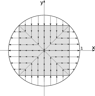
Figure 1: Current density vector field for Example 2.4

The following theorem shows that the equipotential sets contained entirely outside the conductive inclusions are area minimizers. We describe a surface as the level set of a regular map $u$, while competitors are described by level sets of some compact perturbations of the regular map $u$.

Theorem 2.5

(Minimizing property of level sets). Let $\Omega\subset{}^{n}$, $n\geq 2$, be a domain with connected Lipschitz boundary and let $(f,|J|)\in C^{2}(\partial\Omega)\times L^{2}(\overline{\Omega})$ be an admissible pair generated by some unknown $C^{1}$ conductivity. Then for every $v\in C^{2}(\overline{\Omega})$ with $v=f$ on $\partial\Omega$ such that

$$\{x:|\nabla v|=0\}=Z_{v}\cap L_{v},\ \ a(\overline{Z_{v}})=\{0\},$$

where $Z_{v}$ is open and $L_{v}$ has Lebesgue measure zero we have

$${\cal A}(u^{-1}(\lambda))\leq{\cal A}(v^{-1}(\lambda)),$$ (15)

for a.e. $\lambda\in\R$, where $\mathcal{A}$ is defined as $(\ref{massfunctional})$.

The partial data result [45, Theorem 3.4] also recovers the conductivity in two dimensional subregions of type (3) assuming that $|J|>0$ almost everywhere. Below we show that, under the assumption the full vector field $J$ is known (not just its magnitude $|J|$), the partial reconstruction result is valid in three or higher dimensions. The result below can be viewed as the extension of the results in [31] to three or higher dimensional models.

Theorem 2.6

(Partial determination). Let $\Omega\subset{}^{n}$ ($n\geq 2$) be simply connected. For $i=1,2$, let $\sigma^{i}\in C^{\alpha}(\Omega\backslash\overline{U^{i}\cup V^{i}})$ be bounded away from zero, and $u_{i}$ satisfy $(\ref{pde_inclusions})$, where $U^{i}$ and $V^{i}$ are open sets of $\Omega$, and let

$$J_{i}=\left\{\begin{array}[]{ll}\sigma^{i}\nabla u_{i}&\hbox{in}\ \ \Omega\backslash(U^{i}\cup V^{i})\\ 0&\hbox{in}\ \ V^{i}\end{array}\right.$$

For $\alpha<\beta$ let

$$\Omega_{\alpha,\beta}:=\{x\in\overline{\Omega}:\ \ \alpha<u_{1}<\beta\}\ \ \hbox{and}\ \ \Gamma:=\Omega_{\alpha,\beta}\cap\partial\Omega.$$ (17)

Assume that

$$\{x\in\Omega\setminus\overline{U_{1}}:|J_{1}(x)|=0\}=V^{1}\cup W^{1}\cup\Gamma^{1},$$

where $W^{1}$ is open and $\Gamma^{1}$ has Lebesgue measure zero. Then

1. if $u_{1}|_{\Gamma}=u_{2}|_{\Gamma}$ and $J_{1}=J_{2}$ in $\Omega$. Then $U^{1}\cap\Omega_{\alpha,\beta}=U^{2}\cap\Omega_{\alpha,\beta}$, $(W^{1}\cup V^{1})\cap\Omega_{\alpha,\beta}=(W^{2}\cup V^{2})\cap\Omega_{\alpha,\beta}$

   $$u_{1}=u_{2}\ \ \hbox{in}\ \ \Omega_{\alpha,\beta}\backslash V^{1}\ \ \hbox{and}\ \ \sigma^{1}=\sigma^{2}\ \ \hbox{in}\ \ \Omega_{\alpha,\beta}\setminus\overline{U^{1}\cup V^{1}\cup W^{1}}.$$

2. if $u_{1}|_{\Gamma}=u_{2}|_{\Gamma}$ and $J_{1}=J_{2}$ in $\Omega_{\alpha,\beta}$. Then

   $$\{x\in\overline{\Omega}:\ \ \alpha<u_{2}(x)<\beta\}=\Omega_{\alpha,\beta},$$ (18)

   $U^{1}\cap\Omega_{\alpha,\beta}=U^{2}\cap\Omega_{\alpha,\beta}$, $(W^{1}\cup V^{1})\cap\Omega_{\alpha,\beta}=(W^{2}\cup V^{2})\cap\Omega_{\alpha,\beta}$ and

   $$u_{1}=u_{2}\ \ \hbox{in}\ \ \Omega_{\alpha,\beta}\backslash V^{1}\ \ \hbox{and}\ \ \sigma^{1}=\sigma^{2}\ \ \hbox{in}\ \ \Omega_{\alpha,\beta}\setminus\overline{U^{1}\cup V^{1}\cup W^{1}}.$$

Similar to Theorem 2.1 we may determine if an open connected component $O$ of $U^{1}\cup V^{1}\cup W^{1}=U^{2}\cup V^{2}\cup W^{2}$ is a perfectly conducting, insulating, or singular inclusion (see Remark 2.2).

3 Unique determination of the conductivity

In this section we prove Theorems 2.1 and 2.6. The arguments extend those in [44] and [45] by replacing the new admissibility condition. We start with the following proposition.

Proposition 3.1

Let $\Omega\subset{}^{n}$, $n\geq 2$ be a domain and $(f,|J|)\in H^{1/2}(\partial\Omega)\times L^{2}(\Omega)$. Then

1. Assume $(f,|J|)$ is admissible, say generated by some conductivity $\sigma\in L^{\infty}(\Omega\backslash(\overline{U\cup V}))$ where $U$ and $V$ is described in Definition 1 and $u_{0}$ is the corresponding voltage potential. Then $u_{0}$ is a minimizer for $F(u)$ in (2) over

   $$A:=\{u\in H^{1}(\Omega):\ \ u|_{\Omega}=f\}.$$ (19)

   Moreover, if $f\in C^{1,\alpha}(\partial\Omega)$ and if the generating conductivity $\sigma\in C^{\alpha}(\Omega\backslash\overline{U\cup V})$, then the corresponding potential $u_{0}\in C^{1,\alpha}(\Omega\backslash\overline{U\cup V})$ is a minimizer of $F(u)$ over $A$.

2. Assume that the set of zeros of $a=|J|$ can be decomposed as follows

   $$\{x\in\Omega:\ \ a(x)=0\}=V\cup\Gamma_{1},$$

   where $V$ is an open set and $\Gamma_{1}$ has measure zero. Suppose $u_{0}$ is a minimizer for $F(u)$ in (2) over $A$ and the set of zeroes of $|\nabla u_{0}|$ can be decomposed as follows

   $$\{x\in\Omega\setminus V:|\nabla u_{0}|=0\}=\overline{U}\cup\Gamma_{2},$$

   where $U$ is an open set and $\overline{U\cup V}\subset\Omega$, and $\Gamma_{2}$ has measure zero. If $U\cap V=\emptyset$ and $|J|/|\nabla u_{0}|\in L^{\infty}(\Omega\backslash(\overline{U\cup Z}))$ , then $(f,|J|)$ is admissible.

Proof: Assume $(f,|J|)$ is admissible and generated by some conductivity $\sigma\in L^{\infty}_{+}(\Omega\backslash(U\cup V))$. For any $u\in A$ we have

$$F(u) = \int_{\Omega\backslash\overline{(U\cup Z)}}\sigma|\nabla u_{0}||\nabla u|dx+\int_{U}|J||\nabla u|dx$$

$$\geq \int_{\Omega\backslash\overline{(U\cup Z)}}\sigma\nabla u_{0}.\nabla u+\int_{U}|J||\nabla u|dx$$

$$= \int_{\partial\Omega}\sigma\frac{\partial u_{0}}{\partial\nu}uds-\int_{\partial V}\sigma\frac{\partial u_{0}}{\partial\nu}uds-\int_{\partial U}\sigma\frac{\partial u_{0}}{\partial\nu}uds+\int_{U}|J||\nabla u|dx$$

$$= \int_{\partial\Omega}\sigma\frac{\partial u_{0}}{\partial\nu}uds-\int_{\partial U}\sigma\frac{\partial u_{0}}{\partial\nu}uds+\int_{U}|J||\nabla u|dx$$

$$\geq \int_{\partial\Omega}\sigma\frac{\partial u_{0}}{\partial\nu}fds=F(u_{0}).$$

where we have used the admissibility condition (7) and $\nu$ is the outer normal to the boundary of $\Omega$, $U$, and $V$. Hence $u_{0}$ is a minimizer of $F(u)$.

To prove 2) we note that by Lebesgue dominated convergence theorem, the functional $F$ is Gateaux-differentiable at $u\in H^{1}(\Omega)$ with $\frac{|J|}{|\nabla u|}\in L^{\infty}_{+}(\Omega\backslash\overline{(U\cup V)})$. Since

$$F(u_{0})=\int_{\Omega}|J||\nabla u_{0}|=\int_{\Omega\setminus\overline{U\cup V}}|J||\nabla u_{0}|,$$

at a minimizer $u_{0}$ we have

$$F^{\prime}(u_{0})(\varphi)=\int_{\Omega\backslash\overline{U\cup V}}\frac{|J|}{|\nabla u_{0}|}\nabla u_{0}.\nabla\varphi dx=0,$$

for all $\varphi\in W_{0}^{1,1}(\Omega\setminus\overline{U})$. Now let $\sigma=\frac{|J|}{|\nabla u_{0}|}$, then $\nabla.(\sigma\nabla u_{0})=0$ in $\Omega\setminus\overline{V\cup U}$. On the other hand we have

$$\int_{\Omega\backslash\overline{U\cup V}}\frac{|J|}{|\nabla u_{0}|}\nabla u_{0}.\nabla\varphi dx=\int_{\partial(U\cup V)}\sigma\frac{\partial u_{0}}{\partial\nu}\varphi dx=\int_{\partial V}\sigma\frac{\partial u_{0}}{\partial\nu}\varphi dx=0,$$

for all $\varphi\in W_{0}^{1,1}(\Omega\setminus\overline{U})$. Therefore $\frac{\partial u_{0}}{\partial\nu}=0$ on $\partial V$. Now let $O$ be a connected component of $U$. Then for all $\varphi\in W^{1,1}_{0}(\Omega\setminus\overline{U\setminus O})$ with $\varphi\equiv 1$ in $O$ we have

$$\int_{\Omega\backslash\overline{U\cup V}}\frac{|J|}{|\nabla u|}\nabla u_{0}.\nabla\varphi dx=\int_{\partial(U\cup V)}\sigma\frac{\partial u_{0}}{\partial\nu}\varphi dx=\int_{\partial O}\sigma\frac{\partial u_{0}}{\partial\nu}dx=0.$$

This implies that $u_{0}$ is a solution of (5) (see the appendix for more details).

Moreover for every $u\in W^{1,1}_{0}(\Omega)$ with $u|_{\partial\Omega}=f$

$$\int_{\Omega}|J||\nabla u_{0}|dx \leq \int_{\Omega\setminus\overline{V}}|J||\nabla u|dx$$

$$= \int_{U}|J||\nabla u|dx+\int_{\Omega\setminus\overline{U\cup V}}|J||\nabla u|dx$$

$$= \int_{U}|J||\nabla u|dx+\int_{\Omega\setminus\overline{U\cup V}}\sigma|\nabla u_{0}||\nabla u|$$

$$= \int_{U}|J||\nabla u|dx+\int_{\Omega\setminus\overline{U\cup V}}\sigma\nabla u_{0}.\nabla u$$

$$= \int_{U}|J||\nabla u|dx-\int_{\partial U}\sigma\frac{\partial u_{0}}{\partial\nu}udx+\int_{\partial\Omega}\sigma\frac{\partial u_{0}}{\partial\nu}fdx.$$

Since

$$\int_{\Omega}|J||\nabla u_{0}|dx=\int_{\partial\Omega}\sigma\frac{\partial u_{0}}{\partial\nu}fdx,$$

the admissibility condition (7) follows from the above inequality. Thus $(|J|,f)$ is an admissible pair. $\Box$

Now we are ready to prove Theorem 2.1.

Proof of Theorem 2.1: Assume $u_{0}$ is a solution of (5) that corresponds to the admissible pair $(f,|J|)$. It is a direct consequence of the admissibility assumption that

$$\{x\in\Omega:\ \ |J|=0\}\cup\{x\in\Omega:\ \ \nabla u_{\sigma}=0\}=:Z\cup\Gamma,$$

where $Z$ is an open set and $\Gamma$ has measure zero and

$$Z=U\cup V\cup W.$$

Als well, since $\partial(U\cup V)$ is piecewise $C^{1,\alpha}$,

$$u_{0}\in C^{1,\alpha}(\Omega\backslash\overline{U\cup V})\cap C(\Omega\backslash\overline{U\cup V}\cup\partial\Omega)\cap C^{1,\alpha}(\Omega\backslash\overline{U\cup V}\cup T)$$

for every $C^{1,\alpha}$ component of $\partial(U\cup V)$.

By our assumptions $|J|>0$ a.e. in $\Omega\setminus\overline{U\cup V\cup W}$. Hence, equality in (1) yields $|\nabla u_{0}|>0$ a.e. on $\Omega\setminus\overline{U\cup V\cup W}$. Since $U\cup W$ is a disjoint union of countably many connected open sets and $u_{0}$ is constant on every connected open subset of $U\cup W$, the set

$$\Theta:=\{u_{0}(x):\ \ x\in\overline{U\cup W}\}$$

is countable.

Now suppose $u_{1}$ is another minimizer. Then we have

$$\nabla u_{0}=0\ \ \hbox{in}\ \ U\ \ \hbox{and}\ \ \frac{\partial u_{0}}{\partial\nu}=0\ \ \hbox{on}\ \ \partial(V\cup W).$$

Without loss of generality we can assume $u_{0}\geq 0$ in $\overline{\Omega}$. Then

$$F(u_{1}) = \int_{\Omega\setminus\overline{U\cup V\cup W}}\sigma|\nabla u_{0}|.|\nabla u_{1}|dx\geq\int_{\Omega\setminus\overline{U\cup V\cup W}}\sigma|\nabla u_{0}.\nabla u_{1}|dx$$

$$\geq \int_{\Omega\setminus\overline{U\cup V\cup W}}\sigma\nabla u_{0}.\nabla u_{1}=\int_{\partial\Omega}\sigma_{0}\frac{\partial u_{0}}{\partial\nu}u_{1}ds=\int_{\partial\Omega}\sigma_{0}\frac{\partial u_{0}}{\partial\nu}fds$$

$$= F(u_{0}),$$

where $\nu$ is the outer normal to the boundary of $\Omega$. Since $u_{0}$ and $u_{1}$ both minimize the functional $F(u)$, equality holds in (3). On the other hand the equality in Cauchy inequality can only hold for parallel vectors, we have that

$$\nabla u_{1}(x)=\lambda(x)\nabla u_{0}(x),\ \ \ \ \hbox{a.e.}\ \ x\in\Omega\setminus\overline{U\cup V\cup W},$$ (21)

for some Lebesgue- measurable $\lambda(x)$. In particular,

$$\frac{\nabla u_{0}(x)}{|\nabla u_{0}(x)|}=\frac{\nabla u_{1}(x)}{|\nabla u_{1}(x)|}$$ (22)

a.e. on

$$(\Omega\setminus\overline{U\cup V\cup W})\cap\{x\in\Omega:|\nabla u_{1}|\neq 0\}.$$

Let $E_{t}=\{x\in\Omega\setminus\overline{U\cup V\cup W}:u_{0}(x)>t\}$. Since $\Theta$ is countable, for a.e. $t>0$, $\partial E_{t}\cap\overline{(U\cup W)}=\emptyset$ (otherwise $u_{0}$ must be a constant). We claim that the sets $\partial E_{t}\cap(\Omega\setminus\overline{V})$ are smooth $C^{1}$ manifolds in $\Omega\setminus\overline{V}$ for almost all $t>0$ with $\partial E_{t}\cap\overline{U\cup W}=\emptyset$. To prove this note that since $u_{0}\in C^{1}(\Omega\backslash\overline{U\cup V)}$, from equality (22) we have that the measure theoretical normal $\nu_{t}(x)=-\frac{\nabla u_{0}}{|\nabla u_{0}|}$ extends continuously from $\partial^{*}E_{t}\cap(\Omega\backslash\overline{V})$ to the topological boundary $\partial E_{t}\cap(\Omega\backslash\overline{V})$, where $\partial^{*}E_{t}$ is the measure theoretical boundary of $E_{t}$. By the regularity result of De Giorgi (see, e.g. Theorem 4.11 in [18]), we conclude that $\partial E_{t}\cap\Omega\backslash\overline{V}$ is a $C^{1}$-hypersurface for almost all $t>0$.

The function $u_{1}$ is constant on every $C^{1}$ connected components of $\partial E_{t}\cap(\Omega\backslash\overline{V})$. Indeed, let $\gamma:(-\epsilon,+\epsilon)\rightarrow\partial E_{t}\cap(\Omega\backslash\overline{V})$ be an arbitrary $C^{1}$ curve in $\partial E_{t}\cap(\Omega\backslash\overline{V})$. Then we have

$$\frac{d}{dt}u_{1}(\gamma(s))=|\nabla u_{1}(\gamma(s))|\nu(\gamma(s)).\gamma^{\prime}(s)=0,$$

because either $|\nabla u_{1}(\gamma(s))|=0$ or $\nu(\gamma(s)).\gamma^{\prime}(s)=0$ on $\partial E_{t}\cap(\Omega\backslash\overline{V})$. So $u_{1}$ is constant along $\gamma$.

Let $t$ be one of the values for which $\partial E_{t}\cap(\Omega\backslash\overline{V})$ is a hypersurface and $\partial E_{t}\cap\overline{U\cup W}=\emptyset$ (which is the case for almost every $t>0$). We show next that each connected component of $\partial E_{t}$ intersects the boundary $\partial\Omega$.

Arguing by contradiction, assume that $\Sigma_{t}$ is a connected component of $\partial E_{t}$ such that $\Sigma_{t}\cap\partial\Omega=\emptyset$. We consider two cases:

(I) $\Sigma_{t}\cap\partial V=\emptyset$,

(II) $\Sigma_{t}\cap\partial V\neq\emptyset.$

Case I: Assume that $\Sigma_{t}\cap\partial V=\emptyset$. Then $\partial\Omega\cup\Sigma_{t}$ is a compact manifold with two connected components. By the Alexander duality theorem for $\partial\Omega\cup\Sigma_{t}$ (see, e.g., Theorem 27.10 in [19]) we have that ${}^{n}\setminus(\partial\Omega\cup\Sigma_{t})$ is partitioned into three open connected components: ${}^{n}=({}^{n}\setminus\overline{\Omega}\cup O_{1}\cup O_{2})$. Since $\Sigma_{t}\subset\Omega$ we have $O_{1}\cup O_{2}=\Omega\setminus\Sigma_{t}$ and then $\partial O_{i}\subset\partial\Omega\cup\Sigma_{t}$ for $i=1,2$.

We claim that at least one of the $\partial O_{1}$ or $\partial O_{2}$ is in $\Sigma_{t}$. Assume not, i.e. for $i=1,2$, $\partial O_{i}\cap\partial\Omega\neq\emptyset$. Since $\partial\Omega$ is connected (by assumption) we have that $O_{1}\cup O_{2}\cup\partial\Omega$ is connected which implies that $O_{1}\cup O_{2}\cup({}^{n}\setminus\Omega)$ is also connected. Again by applying the Alexander duality theorem for $\Sigma_{t}\subset{}^{n}$, we have that ${}^{n}\setminus\Sigma_{t}$ has exactly two open connected components, one of which is unbounded: ${}^{n}\setminus\Sigma_{t}=O_{\infty}\cup O_{0}$. Since $O_{1}\cup O_{2}\cup({}^{n}\backslash\Omega)$ is connected and unbounded, we have that $O_{1}\cup O_{2}\cup({}^{n}\backslash\Omega)\subset O_{\infty}$, which leaves $O_{0}\subset{}^{n}\setminus(O_{1}\cup O_{2}\cup({}^{n}\setminus\Omega))\subset\Sigma_{t}$. This is impossible since $O_{0}$ is open and $\Sigma_{t}$ is a hypersurface. Therefore either $O_{1}$ or $O_{2}$ or both has the boundary in $\Sigma_{t}$.

Assume $\partial O_{1}\subset\Sigma_{t}$. We claim that $u_{0}=t$ in $O_{1}$. Indeed, since $O_{1}$ is an extension domain ($\partial\Omega_{1}$ has a unit normal everywhere) the new map $\tilde{u_{0}}$ defined by

$$\tilde{u_{0}}:=\left\{\begin{array}[]{ll}u_{0},\ \ x\in\Omega\setminus O_{1},\\ t,\ \ \ \ x\in\overline{O_{1}},\end{array}\right.$$

is in $W^{1,1}(\Omega)\cap C(\overline{\Omega})$ and decreases the functional, which contradicts the minimality of $u_{0}$. Therefore $u_{0}=t$ in $O_{1}$, which makes $|\nabla u_{0}|=0$ in $O_{1}$. This is contradiction since we have assumed $\partial E_{t}\cap\overline{U\cup W}=\emptyset$.

Case (II): Assume $\Sigma_{t}\cap\partial V\neq\emptyset$ and let

$$V_{t}=\{x:\ \ x\in V_{i}\ \ \hbox{and}\ \ V_{i}\cap\Sigma_{t}\neq\emptyset\},$$

where $V_{i}$ are the connected components of $V$. Now define

$$\Sigma^{*}_{t}:=\partial V_{t}\cup\Sigma_{t}.$$

By our assumptions $\Sigma^{*}_{t}$ is a piecewise $C^{1}$-hyperfurface and $\Sigma^{*}_{t}\cap\partial\Omega=\emptyset.$ Since $\partial\Omega\cup\Sigma^{*}_{t}$ is a compact manifold with two connected components, by the Alexander duality theorem and an argument similar to that of case (I) we conclude that $\Omega\backslash\Sigma^{*}_{t}=O_{1}\cup O_{2}$ and at least one of the $\partial O_{1}$ or $\partial O_{2}$ is in $\Sigma^{*}_{t}$. Assume $\partial O_{1}\subset\Sigma^{*}_{t}$ and let

$$O=O_{1}\cap(\Omega\backslash\overline{V}).$$

Then $O$ is a non-empty open subset of $\Omega\backslash\overline{V}$. We claim that $u_{0}=t$ in $O$. Indeed the new map defined by

$$\tilde{u_{0}}:=\left\{\begin{array}[]{ll}u_{0},\ \ x\in\Omega\backslash(V\cup O),\\ t,\ \ \ \ x\in\overline{O},\end{array}\right.$$

can be extended to a function in $W^{1,1}(\Omega)\cap C(\bar{\Omega})$ which decreases the functional and contradics the minimality of $u_{0}$. Hence $u_{0}=t$ in $O$ which is a contradiction because we have assumed $E_{t}\cap\overline{U\cup W}=\emptyset.$

In both cases the contradiction follows from the assumption that $\Sigma_{t}\cap\partial\Omega=\emptyset$. We conclude that each connected component of $\partial E_{t}$ reaches the boundary $\partial\Omega_{t}$. Since $u_{0}$ and $u_{1}$ coincide on the boundary $\partial\Omega$, we have showed that $u_{0}|_{\partial E_{t}}=u_{1}|_{\partial E_{t}}=t$ for almost every $t$. Therefore $u_{0}=u_{1}$ a.e. in $\Omega\setminus\overline{U\cup W}$.

Now note that $u_{0}=u_{1}$ on the boundary of each connected component of $U\cup W$. Since, $u_{0}$ and $u_{1}$ are constant on each connected component of $U\cup W$, $u_{0}$ and $u_{1}$ should also agree on $U\cup W$. Hence $u_{0}=u_{1}$ on $\Omega\setminus V$ and the proof is complete. $\Box$

Proof of Theorem 2.6: To prove the theorem we shall prove the stronger statement 2). It is enough to prove the theorem for each connected component of $\Omega_{\alpha,\beta}$. Hence without loss of generality we may assume that $\Omega_{\alpha,\beta}$ is connected. By the definition of $\Omega_{\alpha,\beta}$ we have

$$u_{1}(\partial\Omega_{\alpha,\beta}\setminus\Gamma)\subset\{\alpha,\beta\}.$$ (25)

Let $J(x):=J_{1}(x)=J_{2}(x)$ for $x\in\Omega_{\alpha,\beta}$. By our assumptions $|J|>0$ a.e. in $\Omega\setminus_{\alpha,\beta}\overline{U^{1}\cup V^{1}\cup W^{1}}$. Hence, $|\nabla u_{1}|>0$ a.e. on $\Omega_{\alpha,\beta}\setminus\overline{U^{1}\cup V^{1}\cup W}$. Since $U^{1}\cup W^{1}$ is a disjoint union of countably many connected open sets and $u_{1}$ is constant on every connected open subset of $U^{1}\cup W$, the set

$$\Theta:=\{u_{1}(x):\ \ x\in\overline{U^{1}\cup W^{1}}\}$$

is countable. Without loss of generality we can assume $u_{1}\geq 0$ in $\Omega_{\alpha,\beta}$.

Since $J_{1}=J_{2}$ in $\Omega_{\alpha,\beta}$, we have that

$$\nabla u_{1}(x)=\lambda(x)\nabla u_{2}(x),\ \ \ \ \hbox{a.e.}\ \ x\in\Omega_{\alpha,\beta}\backslash\overline{U^{1}\cup V^{1}\cup W^{1}},$$ (26)

for some nonnegative Lebesgue-measurable function $\lambda(x)$. In particular, for a.e. $x\in\Omega_{\alpha,\beta}\setminus\overline{U^{1}\cup V^{1}\cup W^{1}}$ we must have

$$\frac{\nabla u_{1}(x)}{|\nabla u_{1}(x)|}=\frac{\nabla u_{2}(x)}{|\nabla u_{2}(x)|}.$$ (27)

Let $E_{t}=\{x\in\Omega_{\alpha,\beta}\setminus\overline{U^{1}\cup V^{1}\cup W^{1}}:u_{1}(x)>t\}$. Since $\Theta$ is countable, for a.e. $t>0$, $\partial E_{t}\cap\overline{U^{1}\cup W^{1}}=\emptyset$ (otherwise $u_{1}$ must be a constant). With an argument similar to that of Theorem 2.1, one can show that the sets $\partial E_{t}\cap(\Omega_{\alpha,\beta}\backslash\overline{V^{1}})$ are smooth $C^{1}$ manifolds in $\Omega_{\alpha,\beta}$ for almost all $t>0$ with $\partial E_{t}\cap\overline{U^{1}\cup W^{1}}=\emptyset$ and the function $u_{2}$ is constant on each connected components of $\partial E_{t}\cap(\Omega_{\alpha,\beta}\backslash\overline{V^{1}})$.

Now let $t\neq\alpha,\beta$ to be one of the values for which $\partial E_{t}\cap(\Omega_{\alpha,\beta}\backslash\overline{V^{1}})$ is a hypersurface and $\partial E_{t}\cap\overline{U^{1}\cup W^{1}}=\emptyset$ (which is the case for almost every $t>0$). We next show that each connected component of $\partial E_{t}$ intersects $\Gamma$.

Arguing by contradiction, assume that $\Sigma_{t}\subset\Omega_{\alpha,\beta}$ is a connected component of $\partial E_{t}$ such that $\Sigma_{t}\cap\partial\Omega=\emptyset$. We consider two cases:

(I) $\Sigma_{t}\cap\partial V^{1}=\emptyset$,

(II) $\Sigma_{t}\cap\partial V^{1}\neq\emptyset.$

Case I: Assume $\Sigma_{t}\cap\partial V^{1}=\emptyset$. Then $\partial\Omega\cup\Sigma_{t}$ is a compact manifold with two connected components. By the Alexander duality theorem we have that ${}^{n}\setminus(\partial\Omega\cup\Sigma_{t})$ is partitioned into three open connected components: ${}^{n}=(({}^{n}\setminus\overline{\Omega})\cup O_{1}\cup O_{2})$. Since $\Sigma_{t}\subset\Omega$ we have $O_{1}\cup O_{2}=\Omega\setminus\Sigma_{t}$ and then $\partial O_{i}\subset\partial\Omega\cup\Sigma_{t}$ for $i=1,2$. With an argument similar to the one provided for the proof of Theorem 2.1, we can show that at least one of the $\partial O_{1}$ or $\partial O_{2}$ is in $\Sigma_{t}$. Assume $\partial O_{1}\subset\Sigma_{t}$. Since $u_{1}$ satisfies the elliptic equation

$$\nabla.(\sigma_{1}\nabla u_{1})=0,\ \ \hbox{in}\ \ O_{1}$$

and $u_{1}=t$ on $\partial O_{1}$, $u_{1}=t$ in $O_{1}$ and therefor $|J|=0$ on $O_{1}$. This is a contradiction since we have assumed $\partial E_{t}\cap\overline{U^{1}\cup W^{1}}=\emptyset$.

Case (II): Assume $\Sigma_{t}\cap\partial V^{1}\neq\emptyset$ and let

$$V_{t}=\{x:\ \ x\in V_{i}^{1}\ \ \hbox{and}\ \ V_{i}\cap\Sigma_{t}\neq\emptyset\},$$

where $V_{i}^{1}$ are the connected components of $V^{1}$. Now define

$$\Sigma^{*}_{t}:=\partial V_{t}\cup\Sigma_{t}.$$

By our assumptions $\Sigma^{*}_{t}$ is a piecewise $C^{1}$-hyperfurface and $\Sigma^{*}_{t}\cap\partial\Omega=\emptyset.$ Since $\partial\Omega\cup\Sigma^{*}_{t}$ is a compact manifold with two connected components, by Alexander duality theorem and an argument similar to that of Theorem 2.1 we conclude that $\Omega\backslash\Sigma^{*}_{t}=O_{1}\cup O_{2}$ and at least one of the $\partial O_{1}$ or $\partial O_{2}$ is in $\Sigma^{*}_{t}$. Assume $\partial O_{1}\subset\Sigma^{*}_{t}$ and let

$$O=O_{1}\cap(\Omega_{\alpha,\beta}\backslash\overline{V^{1}}).$$

Then $O$ is a non-empty open subset of $\Omega_{\alpha,\beta}\backslash\overline{V^{1}}$. We claim that $u_{0}=t$ in $O$. Indeed the new map defined by

$$\tilde{u_{0}}:=\left\{\begin{array}[]{ll}u_{0},\ \ x\in\Omega\backslash(V^{1}\cup O),\\ t,\ \ \ \ x\in\overline{O},\end{array}\right.$$

can be extended to a function in $W^{1,1}(\Omega)\cap C(\bar{\Omega})$ that solves the equation (5). Since the equation (5) has a unique solution $u=\tilde{u}$. Thus $u_{0}=t$ in $O$ which is a contradiction since we have assumed $\partial E_{t}\cap\overline{U^{1}\cup W^{1}}=\emptyset$.

In both cases the contradiction follows from the assumption $\Sigma_{t}\cap\partial\Omega_{\alpha,\beta}=\emptyset$. Since $t\neq\alpha,\beta$ and

$$u_{1}(\partial\Omega_{\alpha,\beta}\setminus\Gamma)\subset\{\alpha,\beta\},$$

$E_{t}$ intersects $\Gamma$ for almost every $t\geq 0$.

Since $u_{0}$ and $u_{1}$ coincide on $\Gamma$, we have showed that $u_{1}|_{\partial E_{t}}=u_{2}|_{\partial E_{t}}=t$ for almost every $t$. Therefore $u_{0}=u_{1}$ a.e. in $\Omega_{\alpha,\beta}\setminus\overline{U^{1}\cup W^{1}}$. Now note that $u_{1}=u_{2}$ on the boundary of each connected component of the set $U^{1}\cup W$. Since, $u_{1}$ and $u_{2}$ are constant on each connected component of $U^{1}\cup W^{1}$, $u_{1}$ and $u_{2}$ should also agree on $U^{1}\cup W$. Hence $u_{1}=u_{2}$ on $\Omega_{\alpha,\beta}\backslash\overline{V^{1}}$. The proof is complete. $\Box$

4 Equipotential surfaces are area minimizing in the conformal metric

In this section we present the proof of Theorem 2.5. We prove that the equipotential sets are global minimizers of $E(\Sigma)$. This is a consequence of minimizing property of the voltage potential for the functional $F(u)$. First we recall the co-area formula.

Theorem 4.1

(Co-area formula). Let $u\in Lip(\Omega)$ and $a$ be integrable in $\Omega\subset{}^{n}$. Then, for a.e. $t\in\R$, $H^{n-1}(u^{-1}(t)\cap\Omega)<\infty$ and

$$\int_{\Omega}a|\nabla u(x)|dx=\int_{-\infty}^{\infty}\int_{u^{-1}(t)}adH^{n-1}(x)dt,$$ (29)

where $H^{n-1}$ is the $(n-1)-$dimensional Hausdorff measure.

Proposition 4.1

Let $a\geq 0$ be integrable in $\Omega$, $U$ be an open subset of $\Omega$, and

$$u\in argmin\left\{\int_{\Omega}a|\nabla v|dx:\ \ v\in Lip(\Omega),\ \ \hbox{and }\ \ v|_{\Omega}=f\right\}.$$

For $\lambda\in\R$ arbitrary fixed, let $u_{+}=\max\{u-\lambda,0\}$ and $u_{-}=\max\{u,\lambda\}$ be defined in $\Omega$, and $f_{+}=\max\{f-\lambda,0\}$, respectively $f_{-}=\min\{f,\lambda\}$, be defined on the boundary $\partial\Omega$. Then

$$u_{+}\in argmin\left\{\int_{\Omega}a|\nabla v|dx:\ \ v\in Lip(\Omega),\ \ \hbox{and }\ \ v|_{\Omega}=f_{+}\right\},$$

and

$$u_{-}\in argmin\left\{\int_{\Omega}a|\nabla v|dx:\ \ v\in Lip(\Omega),\ \ \hbox{and }\ \ v|_{\Omega}=f_{-}\right\}.$$

Proof: The proof is similar to the proof of Proposition 2.2 [45] and we omit it. $\Box$

Corollary 4.2

Let $a\geq 0$ be integrable in $\Omega$, $U$ be an open subset of $\Omega$, and

$$u\in argmin\left\{\int_{\Omega}a|\nabla v|dx:\ \ v\in Lip(\Omega),\ \ \hbox{and }\ \ v|_{\Omega}=f\right\}.$$

For every $\lambda\in\R$ and $\epsilon>0$ define

$$u_{\lambda,\epsilon}:=\frac{1}{\epsilon}\min\{\epsilon,\max\{u-\lambda,0\},\}$$ (30)

and let $f_{\lambda,\epsilon}$ be its trace on the boundary $\partial\Omega$. Then $u_{\lambda,\epsilon}\in Lip(\Omega)$ and

$$u_{\lambda,\epsilon}\in argmin\left\{\int_{\Omega}a|\nabla v|dx:\ \ v\in Lip(\Omega),\ \ \hbox{and}\ \ v|_{\Omega}=f_{\lambda,\epsilon}\right\}.$$

Proof: The proof follows directly from Proposition 4.1 applied twice. $\Box$

Lemma 4.3

Let $a,u\in Lip(\Omega)$ such that

$$\{x:\ \ |\nabla u(x)|=0\}=Z\cup L,$$

where $Z$ is open and $L$ has Lebesgue measure zero, $a(\overline{Z})=\{0\}$, and

$$a\frac{\nabla u}{|\nabla u|}\in W^{1,1}(\Omega\backslash\overline{Z}).$$ (31)

Then for almost every $\lambda\in\R$,

$$\lim_{\epsilon\rightarrow 0}\int_{\Omega}a|\nabla u_{\lambda,\epsilon}|dx=\int_{u^{-1}(\lambda)}adH^{n-1}(x),$$ (32)

where $u_{\lambda,\epsilon}$ is defined by $(\ref{u.ep})$.

Proof. The proof is similar to the proof of Lemma 2.4 in [45]. From Theorem 4.1, we have $H^{n-1}(u^{-1}(\lambda)\cap\Omega)<\infty$, a.e. $\lambda\in\R$. In particular

$$H^{n}(u^{-1}(\lambda)\cap\Omega)=0.$$ (33)

Since $H^{n-1}(\partial\Omega)<\infty$, from the disjoint partition $\partial\Omega=\bigcup_{\lambda\in\R}(u^{-1}(\lambda)\cap\partial\Omega)$, we have

$$H^{n-1}(u^{-1}(\lambda)\cap\partial\Omega)>0,$$

for at most countable many $\lambda$. In particular, for almost every $\lambda\in\R$

$$H^{n-1}(u^{-1}(\lambda)\cap\partial\Omega)=0.$$ (34)

Let $\lambda\in Range(u)$ be such that both (33) and (34) hold, and $\epsilon>0$. Recall

$$u_{\lambda,\epsilon}=\left\{\begin{array}[]{ll}0&\hbox{if}\ \ u(x)<\lambda,\\ (u(x)-\lambda)/\epsilon&\hbox{if}\ \ \lambda\leq u(x)\leq\lambda+\epsilon,\\ 0&\hbox{if}\ \ u(x)>\lambda+\epsilon.\end{array}\right.$$

From the co-area formula we have

$$\int_{\Omega}a|\nabla u_{\lambda,\epsilon}|dx = \int_{-\infty}^{+\infty}\int_{(u_{\lambda,\epsilon})^{-1}(t)}adH^{n-1}(x)dt$$ (36)

$$= \int_{0}^{1}\int_{\{x:\ \ u(x)=\lambda+t\epsilon\}}adH^{n-1}(x)$$

To complete the proof it is enough to prove that

$$\lim_{\epsilon\rightarrow 0}\int_{\{x:u(x)=\lambda+\epsilon\}}adH^{n-1}(x)=\int_{\{x:u(x)=\lambda\}}adH^{n-1}(x),$$ (37)

holds uniformly for almost every $t\in[0,1]$. The domain

$$\Omega_{t,\epsilon}:=\{x\in\Omega:\lambda<u(x)<\lambda+t\epsilon\}$$

is Lipschitz. Since $a\in Lip(\Omega)$, it extends continuously to the boundary. The $a\nabla u/|\nabla u|\in W^{1,1}(\Omega\backslash\overline{Z})$ also extends to the boundary $\partial(\Omega\backslash Z)$ as a bounded function. Now notice that $u(\overline{Z})$ is at most countable. Therefore, for a. e. $\lambda\in Range(u)$ and a.e. $t\in[0,1]$ the outer unit normal $\nu$ to the boundary $\partial\Omega_{t,\epsilon}$ exists. Then Green’s formula in $\Omega_{t,\epsilon}$ yields

$$|\int_{u^{-1}(\lambda+t\epsilon)}adH^{n-1}-\int_{u^{-1}(\lambda)}adH^{n-1}|$$

$$= |\int_{u^{-1}(\lambda+t\epsilon)\cap\Omega\backslash{\overline{Z}}}adH^{n-1}-\int_{u^{-1}(\lambda)\cap\Omega\backslash{\overline{Z}}}adH^{n-1}|$$

$$\leq |\int_{\{x\in\partial\Omega:\ \ \lambda<u(x)<\lambda+\epsilon\}}a\frac{\nabla u}{|\nabla u|}\nu dH^{n-1}(x)|$$

$$+ |\int_{\{x\in\Omega:\ \ \lambda<u(x)<\lambda+\epsilon\}}\nabla.a\frac{\nabla u}{|\nabla u|}dx|.$$

Using (33) we have

$$\lim_{\epsilon\rightarrow 0}H^{n}(\{x\in\Omega:\lambda<u(x)<\lambda+\epsilon\}) = H^{n}(\bigcap_{\epsilon>0}\{x\in\Omega:\lambda<u(x)<\lambda+\epsilon\})$$

$$\leq H^{n}(\bigcap_{\epsilon>0}\{x\in\Omega:\lambda\leq u(x)<\lambda+\epsilon\})$$

$$= H^{n}(u^{-1}(\lambda)\cap\Omega)=0.$$

Similarly by (34) we obtain

$$\lim_{\epsilon\rightarrow 0}H^{n-1}(\{x\in\partial\Omega:\lambda<u(x)<\lambda+\epsilon\})=0.$$

This proves (37). By taking the limit $\epsilon\rightarrow 0$ in (36) and using (37) we obtain (32). $\Box$

Proof of Theorem 2.5: For $\lambda\not\in Range(u)$, the left hand side of (15) is zero and and the inequality trivially holds. Since $u$ obeys the maximum principle and $u=v$ on $\partial\Omega$, $Range(u)\subset Range(v)$.

Now let $\lambda\in Range(u)\setminus\left(u(\overline{Z})\cup v(\overline{Z_{v}})\right)$ and recall that $u(\overline{Z})$ and $u(\overline{Z_{v}})$ are both countable. Since $|\nabla u|\neq 0$ a.e. in $\Omega\setminus\overline{Z}$ and $|\nabla v|\neq 0$ a.e. in $\Omega\setminus\overline{S_{v}}$, for almost every $\lambda\in Range(u)$ the corresponding $\lambda-$level set is a $C^{1}$-smooth oriented surface. In particular the $H^{n-1}-$measure coincides with the induced Lebesgue measure on the respective surface. Moreover, $u$ and $v$ satisfy $(\ref{n.m })$ and $(\ref{(n-1).m})$ for a.e. $\lambda\in\R$.

For $\epsilon>0$ arbitrary fixed, let $u_{\lambda,\epsilon}$ be defined by (30) and define similarly

$$v_{\lambda,\epsilon}:=\min\{\epsilon,\max\{v-\lambda,0\}/\epsilon\}.$$

Since $u=v$ on the boundary $\partial\Omega$, we also have $u_{\lambda,\epsilon}=v_{\lambda,\epsilon}$ on $\partial\Omega$. From Corollary 4.2 we have

$$\int_{\Omega}a|\nabla u_{\lambda,\epsilon}|dx\leq\int_{\Omega}a|\nabla v_{\lambda,\epsilon}|dx.$$ (38)

Letting $\epsilon\rightarrow 0$ and applying Lemma 4.3 we obtain (15). $\Box$

5 Appendix: Perfectly conductive and insulating inclusions

The results in this appendix formalize the definition of perfectly conducting as infinity limit of conductivity. They are slight generalization of the ones in [8] to include both perfectly conductive and insulating inclusions.

Let $U=\cup_{j=1}^{\infty}U_{j}$ be an open subset of $\Omega$ with $\overline{U}\subset\Omega$ to model the union of the connected components $U_{j}$ ($j=1,2,...$) of perfectly conductive inclusions, and $V$ be an open subset of $\Omega$ with $\overline{V}\subset\Omega$ to model the union of all connected insulating inclusions. Let $\chi_{U}$ and $\chi_{V}$ be their corresponding characteristic function. We assume that $\overline{U}\cap\overline{V}=\emptyset$, $\Omega\setminus\overline{U\cup V}$ is connected, and that the boundaries $\partial U$, $\partial V$ are piecewise $C^{1,\alpha}$. Let $\sigma_{1}\in L^{\infty}(U)$, and $\sigma\in L^{\infty}(\Omega\setminus\overline{U\cup V})$ be such that

$$0<\lambda\leq\sigma_{1},\sigma\leq\Lambda<\infty,$$ (39)

for some positive constants $\lambda$ and $\Lambda$.

For each $0<k<1$ consider the conductivity problem

$$\nabla\cdot(\chi_{U}(\frac{1}{k}\sigma_{1}-\sigma)+\sigma)\nabla u=0,\qquad\frac{\partial u}{\partial\nu}=0\ \hbox{on}\ \ \partial V,\ \ \hbox{and}\qquad u|_{\partial\Omega}=f.$$ (40)

The condition on $\partial V$ ensures that $V$ is insulating. It is well known that the problem (40) has a unique solution $u_{k}\in H^{1}(\Omega)$ which also solves:

$$\left\{\begin{array}[]{ll}\nabla\cdot\sigma\nabla u_{k}=0,&\mbox{in}\,\Omega\setminus\overline{U\cup V},\\ \nabla\cdot\sigma_{1}\nabla u_{k}=0,&\mbox{in}\,U,\\ u_{k}|_{+}=u_{k}|_{-},&\mbox{on}\,\partial U,\\ \left.\frac{1}{k}\sigma_{1}\frac{\partial u_{k}}{\partial\nu}\right|_{-}=\left.\sigma\frac{\partial u_{k}}{\partial\nu}\right|_{+},&\mbox{on}\,\partial U,\\ \left.\frac{\partial u_{k}}{\partial\nu}\right|_{+}=0,&\mbox{on}\,\partial V,\\ u_{k}|_{\partial\Omega}=f.\end{array}\right.$$ (41)

Moreover, the energy functional

$$I_{k}[v]=\frac{1}{2k}\int_{U}\sigma_{1}|\nabla v|^{2}dx+\frac{1}{2}\int_{\Omega\setminus\overline{U\cup V}}\sigma|\nabla v|^{2}dx$$ (42)

has a unique minimizer over the maps in $H^{1}(\Omega)$ with trace $f$ at $\partial\Omega$ which is the unique solution $u_{k}$ of (41).

We shall show below why the limiting solution (with $k\to 0$) solves

$$\left\{\begin{array}[]{ll}\nabla\cdot\sigma\nabla u_{0}=0,&\mbox{in}\,\Omega\setminus\overline{U\cup V},\\ \nabla u_{0}=0,&\mbox{in}\ \ U,\\ u_{0}|_{+}=u_{0}|_{-},&\mbox{on}\ \ \partial U,\\ \int_{\partial U_{j}}\sigma\frac{\partial u_{0}}{\partial\nu}|_{+}ds=0,&j=1,2,...,\\ \frac{\partial u_{0}}{\partial\nu}|_{+}=0,&\mbox{on}\;\partial V,\\ u_{0}|_{\partial\Omega}=f,\\ \end{array}\right.$$ (43)

By elliptic regularity $u_{0}\in C^{1,\alpha}(\Omega\backslash U\cup V)$ and for any $C^{1,\alpha}$ boundary portion $T$ of $\partial(U\cup V)$, $u_{0}\in C^{1,\alpha}((\Omega\backslash(U\cup V))\cup T)$.

Proposition 5.1

The problem (43) has a unique solution in $H^{1}(\Omega)$ which is the unique minimizer of the functional

$$I_{0}[v]=\frac{1}{2}\int_{\Omega\setminus\overline{U\cup V}}\sigma|\nabla v|^{2}dx,$$ (44)

over the set $A_{0}:=\{u\in H^{1}(\Omega\setminus\overline{V});\,u|_{\partial\Omega}=f,\,\nabla u=0\,\mbox{in}\,U\}$.

Proof: Note that $A_{0}$ is weakly closed in $H^{1}(\Omega\setminus\overline{V})$. The functional $I_{0}$ is lower semicontinuous, strictly convex, and, thus, has a unique minimizer $u_{0}^{*}$ in $A_{0}$.

First we show that $u_{0}^{*}$ is a solution of (43). Since $u_{0}^{*}$ minimizes (44), we have

$$0=\int_{\Omega\setminus\overline{V\cup U}}\sigma\nabla u^{*}_{0}\cdot\nabla{\varphi}dx,$$ (45)

for all ${\varphi}\in H^{1}(\Omega\setminus\bar{V})$, with ${\varphi}|_{\partial\Omega}=0$, and $\nabla{\varphi}=0$ in $U$. In particular, if ${\varphi}\in H^{1}_{0}(\Omega\setminus\bar{V})$, we get $\int_{\Omega\setminus\overline{U\cup V}}(\nabla\cdot\sigma\nabla u_{0}^{*}){\varphi}dx=0$ and thus $u_{0}^{*}$ solves the conductivity equation in (43). If we choose ${\varphi}\in H^{1}(\Omega\setminus\bar{V})$, with ${\varphi}|_{\partial\Omega}=0$, and ${\varphi}\equiv 0$ in $U$, from Green’s formula applied to (45), we get $\int_{\partial V}\sigma\left.\frac{\partial u_{0}^{*}}{\partial\nu}\right|_{+}{\varphi}=0,\,\forall\,{\varphi}|_{\partial V}\in H^{1/2}(\partial V),$ or, equivalently, $\sigma\left.\frac{\partial u_{0}^{*}}{\partial\nu}\right|_{\partial V}=0$. If we choose ${\varphi}_{j}\in H^{1}_{0}(\Omega\setminus\bar{V})$ with ${\varphi}_{j}\equiv 1$ in the connected component $U_{j}$ of $U$ and ${\varphi}_{j}\equiv 0$ in $U\setminus U_{j}$, from Green’s formula applied to (45) we obtain $\int_{\partial U_{j}}\sigma\frac{\partial u_{0}^{*}}{\partial\nu}=0$.

Next we show that the equation (43) has a unique solution and, consequently, $u_{0}^{*}=u_{0}|_{\Omega\setminus\overline{V}}$. Assume that $u^{1}$ and $u^{2}$ are two solutions and let $u=u_{2}-u_{1}$, then $u|_{\partial\Omega}=0$ and

$$0= -\int_{\Omega\setminus\overline{U\cup V}}(\nabla\cdot\sigma\nabla u)udx=-\int_{\partial\Omega}\sigma\frac{\partial u}{\partial\nu}uds+\int_{\partial V}\sigma\left.\frac{\partial u}{\partial\nu}\right|_{+}uds$$ (46)

$$+\int_{\partial U}\sigma\left.\frac{\partial u}{\partial\nu}\right|_{+}uds+\int_{\Omega\setminus\overline{U\cup V}}\sigma|\nabla u|^{2}dx=\int_{\Omega\setminus\overline{U\cup V}}\sigma|\nabla u|^{2}dx.$$ (47)

Since $\sigma\geq\lambda>0$, we get $|\nabla u|=0$ in $\Omega\setminus\overline{V}$. Since $\Omega\setminus\overline{V}$ is connected and $u=0$ at the boundary, we conclude uniqueness of the solution of the equations (43). $\Box$

Theorem 5.1

Let $u_{k}$ and $u_{0}$ be the unique solution of (41) respectively (43) in $H^{1}(\Omega)$. Then $u_{k}\rightharpoonup u_{0}$ and, consequently, $I_{k}[u_{k}]\to I_{0}[u_{0}]$ as $k\to 0^{+}$.

Proof: We show first that $\{u_{k}\}$ is bounded in $H^{1}(\Omega)$ uniformly in $k\in(0,1)$. Since $1/k>1$, we have

$$\frac{\lambda}{2}\|\nabla u_{k}\|^{2}_{L^{2}(\Omega\setminus\overline{V})}\leq\frac{1}{2}\int_{\Omega\setminus\overline{U\cup V}}\sigma|\nabla u_{k}|^{2}dx+\frac{1}{2k}\int_{U}\sigma_{2}|\nabla u_{k}|^{2}dx$$

$$\leq I_{k}[u_{k}]\leq I_{k}[u_{0}]\leq\frac{\Lambda}{2}\|\nabla u_{0}\|^{2}_{L^{2}(\Omega\setminus\overline{V})},$$

or

$$\|\nabla u_{k}\|^{2}_{L^{2}(\Omega\setminus\overline{V})}\leq\frac{\Lambda}{\lambda}\|\nabla u_{0}\|^{2}_{L^{2}(\Omega\setminus\overline{V})}.$$ (48)

From (48) and the fact that $u_{k}|_{\partial\Omega}=f$, we see that $\{u_{k}\}$ is uniformly bounded in $H^{1}(\Omega\backslash V)$ and hence weakly compact. Therefore, on a subsequence $u_{k}\rightharpoonup u_{0}^{*}$ in $H^{1}(\Omega\backslash V)$, for some $u_{0}^{*}$ with trace $f$ at ${\partial\Omega}$.

We will show next that $u_{0}^{*}$ satisfies the equations (43), and therefore $u_{0}^{*}=u_{0}$ on $\Omega$. By the uniqueness of solutions of (43) we also conclude that the whole sequence converges to $u_{0}$.

Since $u_{k}\rightharpoonup u_{0}^{*}$ we have that $0=\int_{\Omega\setminus\overline{U\cup V}}\sigma\nabla u_{k}\cdot\nabla{\varphi}dx\to\int_{\Omega\setminus\overline{U\cup V}}\sigma_{2}\nabla u_{0}^{*}\cdot\nabla{\varphi}dx$, for all ${\varphi}\in C^{\infty}_{0}({\Omega\setminus\overline{U\cup V}})$. Therefore $\nabla\cdot\sigma\nabla u_{0}^{*}=0$ in ${\Omega\setminus\overline{U\cup V}}$. Also because $u_{k}$ is a minimizers of $I[u_{k}]$ we must have $\nabla u_{0}^{*}=0$ in $U$. To check the boundary conditions, note that, for all ${\varphi}\in C^{\infty}_{0}(\Omega)$ with ${\varphi}\equiv 0$ in $U$, we have $\int_{\partial V}\sigma\left.\frac{\partial u_{k}}{\partial\nu}\right|_{+}{\varphi}ds=0$. Using the fact that ${\varphi}$ were arbitrary, by taking the weak limit in $k\to 0$, we get $\left.\frac{\partial u_{0}^{*}}{\partial\nu}\right|_{+}=0$ on $\partial V$. A similar argument applied to ${\varphi}\in C^{\infty}_{0}(\Omega)$ with ${\varphi}\equiv 0$ in $V$, ${\varphi}\equiv 1$ in $U_{j}$, and ${\varphi}\equiv 0$ in $U\backslash U_{j}$, also shows that $\int_{\partial{U_{j}}}\sigma\left.\frac{\partial u_{0}^{*}}{\partial\nu}\right|_{+}{\varphi}ds=0$. Hence $u^{*}_{0}$ is the unique solution of the equation (43) on $\Omega\backslash\overline{V}$. Thus $u_{k}$ converges weakly to the solution $u_{0}$ of (43) in $\Omega\backslash\overline{V}$. $\Box$

References

• [1] G. Alessandrini, An identification problem for an elliptic equation in two variables, Annali di matematica pura ed applicata, 145 (1986), pp. 265–295.
• [2] H. Ammari, Y. Capdeboscq, H. Kang, and A. Kozhemiak, Mathematical models and reconstruction methods in magneto-acouostic imaging, European J. Appl. Math., 20(2009), pp. 303–317.
• [3] H. Ammari, E. Bonnetier, Y. Capdeboscq, M. Tanter, and M. Fink, Electrical Impedance Tomography by Elastic Deformation, SIAM J. Appl. Math., 68 (2008), pp.1557–1573.
• [4] Habib Ammari, Josselin Garnier, Hyonbae Kang, Won-Kwang Park, and Knut Solna, Imaging Schemes for Perfectly Conducting Cracks, SIAM J. Appl. Math., 71 (2011), pp.68–91.
• [5] G. Bal and J.C. Schotland, Inverse Scattering and Acousto-Optic Imaging, Phys. Rev. Letters 104(2010), 043902.
• [6] G. Bal, Hybrid inverse problems and internal information, preprint (2011).
• [7] G. Bal and G. Uhlmann, Inverse Diffusion Theory of Photoacoustics, Inverse Problems 26(2010), 085010.
• [8] E. S. Bao, Y. Y. Li, and B. Yin Gradient estimates for the perfect conductivity problem, Arch. Rational Mech. Anal. 193 (2009), 195–226.
• [9] , L. Bers, F. John, and M. Schechter, Partial Differential Equations, Wileys & Sons, New York, 1964.
• [10] E. Bombieri, E. De Giorgi and E. Giusti, Minimal Cones and the Bernstein Problem, Inventiones Math. 7 (1969), pp. 243–268.
• [11] L. Borcea, Electrical impedance tomography, Inverse Problems 18(2002), R99–R136.
• [12] M. Cheney, D. Isaacson, and J. C. Newell, Electrical Impedance Tomography, SIAM Rev. 41(1999), no.1, 85 –101.
• [13] B. T. Cox, S. R. Arridge, K. P. Kostli, and P. C.Beard,2D quantitative photoacoustic image reconstruction of absorption distributions in scattering media using a simple iterative method, Applied Optics 45(2006), 1866–1875.
• [14] M. G. Crandall, H. Ishii, and P. -L. Lions User’s guide to viscosity solutions of second order partial differential equations,Bull. Amer. Math. Soc. 27(1992), 1–67.
• [15] D. Isaacson and M. Cheney, Effects of measurement precision and finite numbers of electrodes on linear impedance imaging algorithms, SIAM J. Appl. Math. 51 (1991), no. 6, 1705–1731.
• [16] B. Gebauer and O. Scherzer, Impedance-acoustic tomography, SIAM J. Appl. Math., 69 (2008), pp. 565–576.
• [17] A. Greenleaf, Y. Kurylev, M. Lassas, and G. Uhlmann, Invisibility and inverse problems, Bull. Amer. Math. Soc. 46 (2009), 55-97.
• [18] E. Giusti, Minimal Surfaces and Funcitons of Bounded Variations, 1984 (Boston: Birkh╝user).
• [19] J. M. Greenberg and J. R. Harper, Algebraic Topology, 1981 (Benjamin - Cummings).
• [20] K. F. Hasanov, A. W. Ma, A. I. Nachman, and M. J. Joy, Current Density Impedance Imaging, IEEE Trans. Med. Imag. 27(2008),pp. 1301–1309.
• [21] Y.Z. Ider and Ö. Birgül , Use of the magnetic field generated by the internal distribution of injected currents for Electrical Impedance Tomography(MR-EIT), Elektrik 6 (1998), 215–225
• [22] L. Ji, J. R. McLaughlin, D. Renzi and J.-R. Yoon, Interior elastodynamics inverse problems: shear wave speed reconstruction in transient elastography, Inverse Problems 19(2003), S1朣29.
• [23] M. L. Joy, G. C. Scott, and M. Henkelman, In vivo detection of applied electric currents by magnetic resonance imaging, Magnetic Resonance Imaging, 7 (1989), pp. 89–94.
• [24] M. J. Joy, A. I. Nachman, K. F. Hasanov, R. S. Yoon, and A. W. Ma, A new approach to Current Density Impedance Imaging (CDII), Proceedings ISMRM, No. 356, Kyoto, Japan, 2004.
• [25] H.S. Khang, B.I. Lee, S. H. Oh, E.J. Woo, S. Y. Lee, M.H. Cho, O. I. Kwon, J.R. Yoon, and J.K. Seo, J-substitution algorithm in magnetic resonance electrical impedance tomography (MREIT): Phantom experiments for static resistivity images, IEEE Trans. Med. Imag., 21(2002), no. 6, pp. 695 –702.
• [26] S. Kim, O. Kwon, J. K. Seo, and J. R. Yoon, On a nonlinear partial differential equation arising in magnetic resonance electrical impedance tomography, SIAM J. Math. Anal., 34 (2002), pp. 511–526.
• [27] Y.J. Kim, O. Kwon, J. K. Seo, and E. J. Woo, Uniqueness and convergence of conductivity image reconstruction in magnetic resonance electrical impedance tomography, Inverse Problems 19(2003), no. 5, 1213- 25.
• [28] P. Kuchment and L. Kunyansky, 2D and 3D reconstructions in acousto-electric tomography, preprint.
• [29] O. Kwon, E. J. Woo, J. R. Yoon, and J. K. Seo, Magnetic resonance electric impedance tomography (MREIT): Simulation study of J-substitution algorithm, IEEE Trans. Biomed. Eng., 49 (2002), pp. 160–167
• [30] O. Kwon, C. J. Park, E.J. Park, J. K. Seo, and E. J. Woo , Electrical conductivity imaging using a variational method in $B_{z}$-based MREIT, Inverse Problems 21 (2005), pp. 969–980.
• [31] O. Kwon, J. Y Lee, and J. R. Yoon, Equipotential line method for magnetic resonance electrical impedance tomography, Inverse Problems 18 (2002), pp. 1089- 00
• [32] J. Y. Lee A reconstruction formula and uniqueness of conductivity in MREIT using two internal current distributions, Inverse Problems 20 (2004), pp. 847–858
• [33] X. Li, Y. Xu and B. He, Imaging Electrical Impedance from Acoustic Measurements by Means of Magnetoacoustic Tomography with Magnetic Induction (MAT-MI), IEEE Trans. Biomed. Eng. 54(2007), pp. 323 330.
• [34] A. Liseno and R. Pierri Imaging perfectly conducting objects as support of induced currents: Kirchhoff approximation and frequency diversity, Journal of the Optical Society of America A, Vol. 19, Issue 7, pp. 1308-1318 (2002).
• [35] J. J. Liu, H. C. Pyo, J. K. Seo, and E. J. Woo, Convergence properties and stability issues in MREIT algorithm, Contemporaty Mathematics 25 (2006), 168–176.
• [36] J. J. Liu, J. K. Seo, M. Sini and E. J. Woo, On the convergence of the harmonic Bz Algorithm in Magnetic Resonance Imaging, SIAM J. Appl. Math. 67 (2007), 1259–1282.
• [37] J. J. Liu, J. K. Seo, and E. J. Woo, A Posteriori Error Estimate and Convergence Analysis for Conductivity Image Reconstruction in MREIT, SIAM J. Appl. Math. 70(2010), Issue 8, pp. 2883–2903.
• [38] Q. Ma and B. He, Investigation on magnetoacoustic signal generation with magnetic induction and application to electrical conductivity reconstruction, Phys. Med. Biol., 52 (2007), pp. 5085–5099.
• [39] J. Malý, D. Swanson, and W. P. Ziemer, The co-area formula for Sobolev mappings, Trans. Amer. Math. Soc. 355(2003), no. 2, 477 492.
• [40] N. Mandache, Exponential instability in an inverse problem for the Schr鰀inger equation, Inverse Problems 17 (2001), pp. 1435–1444.
• [41] O. Martio, Counterexamples for unique continuation, Manuscripta Math. 60(1988), pp. 21 .
• [42] J. R. McLaughlin and J. -R. Yoon, Unique identifiability of elastic parameters from time-dependent interior displacement measurement, Inverse Problems20(2004), pp. 25-46.
• [43] A. Nachman, A. Tamasan, and A. Timonov, Conductivity imaging with a single measurement of boundary and interior data, Inverse Problems, 23 (2007), pp. 2551–2563.
• [44] A. Nachman, A. Tamasan, and A. Timonov, Recovering the conductivity from a single measurement of interior data, Inverse Problems, 25 (2009) 035014 (16pp).
• [45] A. Nachman, A. Tamasan, and A. Timonov, Reconstruction of Planar Conductivities in Subdomains from Incomplete Data, SIAM J. Appl. Math. 70(2010), Issue 8, pp. 3342–3362.
• [46] A. Nachman, A. Tamasan, and A. Timonov, Current density impedance imaging, preprint (2011).
• [47] M. Z. Nashed and A. Tamasan, Structural stability in a minimization problem and applications to conductivity imaging, Inverse Probl. Imaging, 4 (2010) to appear.
• [48] S.H. Oh, B. I. Lee, E. J. Woo, S. Y. Lee, M. H. Cho, O. Kwon, and J. K. Seo, Conductivity and current density image reconstruction using $B_{z}$ algorithm in magnetic resonance electrical impedance tomography, Phys. Med. Biol. 48(2003), pp. 3101–3116.
• [49] S. Onart, Y.Z. Ider, and W. Lionheart, Uniqueness and reconstructions in magnetic resonance -electrical impedance tomography (MR-EIT), Physiol. Meas. 24(2003), pp. 591–604.
• [50] C. Park, O. Kwon, E.J. Woo, and J. K. Seo, ELectrical conductivity imaging using gradient $B_{z}$ decomposition algorithm in magnetic resonance electrical impedance tomography (MREIT), IEEE Trans. Med. Imag. 23(2004), pp. 388–394.
• [51] A. Plis, One non-uniquness in Cauchy problem for an elliptic second orde differantial equation, Bull. Acad. Pol. Sci., S. Mat. XI(1963), pp. 95-100.
• [52] G. C. Scott, NMR imaging of current density and magnetic fields, Ph.D. dissertation, Univ. Toronto, Toronto, Canada, 1993.
• [53] G. C. Scott, M. L. Joy, R. L. Armstrong, and R. M. Henkelman, Measurement of nonuniform current density by magnetic resonance, IEEE Trans. Med. Imag., 10 (1991), pp. 362–374
• [54] P. Sternberg and W. P. Ziemer, Generalized motion by curvature with a Dirichlet condition, J. Differ. Eq., 114(1994), pp. 580–600.
• [55] P. Sternberg and W. P. Ziemer, The Dirichlet problem for functions of least gradient. Degenerate diffusions (Minneapolis, MN, 1991), 197–214, in IMA Vol. Math. Appl., 47, Springer, New York, 1993.
• [56] E. J. Woo and J. K. Seo, Magnetic resonance electrical impedance tomography (MREIT) for high resolution conductivity imaging, Physiol. Meas., 29 (2008), pp. R1-R26.
• [57] L. V. Wang, Prospects of photoacoustic tomography, Medical Physics35(2008), 5758 5767.
• [58] N. Zhang, Electrical impedance tomography based on current density imaging, M.Sc. Thesis: University of Toronto, Canada, 1992.