Superradiance in spin-$J$ particles: Effects of multiple levels

Abstract

We study the superradiance dynamics in a dense system of atoms each of which can be generally a spin-$j$ particle with $j$ an arbitrary half-integer. We generalize Dicke’s superradiance point of view to multiple-level systems, and compare the results based on a novel approach we have developed in [Yelin et al., arXiv:quant-ph/0509184]. Using this formalism we derive an effective two-body description that shows cooperative and collective effects for spin-$j$ particles, taking into account the coherence of transitions between different atomic levels. We find that the superradiance, which is well-known as a many-body phenomenon, can also be modified by multiple level effects. We also discuss the feasibility and propose that our approach can be applied to polar molecules, for their vibrational states have multi-level structure which is partially harmonic.

I Introduction

Quantum many-body physics has been one of the most attractive areas for decades along with the remarkable advents in the fields of ultracold atomic and molecular systems and quantum optics. These systems not only provide an excellent testbed to study quantum nature of various many-body phenomena such as Bose-Einstein condensation, superfluidity Sci95_Anderson ; Nat03_Greiner ; RMP01_Leggett , quantum magnetism, and quantum phase transitions PRB89_Fisher ; Nat02_Greiner ; Nat06_Hadzibabic ; PRL08_Weimer , but also inspire the implementation of quantum machinery such as quantum simulation PRL03_Duan ; PRL04_Porras ; NatPhys08_Friedenauer ; Nat10_Gerritsma ; Nat10_Kim ; Nat09_Lin and quantum computing PRL99_Brennen ; Kuznetsova11a ; Kuznetsova11b . In many ways, quantum many-body effects are “exotic” compared to their classical counterparts, and even to quantum single-body physics, mainly due to particle statistics and indistinguishability of particles. The circumstances can become even more complicated when an ensemble of particles interact cooperatively which results in higher-order nonlinear effects. Superradiance, usually representing an $N^{2}$ enhancement of the radiation intensity due to coherent decay of a dense sample consisting of $N$ excited atoms, is one important example which can be understood qualitatively through particle indistinguishability and symmetry arguments without the need for considering particle statistics. This phenomenon was first predicted in 1954 by R. H. Dicke PhysRev54_Dicke , who pointed out that the radiative properties of an excited atom can be very different just because other atoms are present or not, given that their distance is much smaller than the wavelength of the radiation field even if the particle wavepackets do not overlap and no direct interaction is present. Since then such cooperative effects have been intensively investigated both theoretically and experimentally PhysLett74_DeMartini ; PhysRep82_Gross ; Sci99_Inouye ; PRL99_Moore ; PRA00_Mustecaplioglu ; PRL03_Farooqi ; PRL08_Akkermans . Recently, superradiance re-catches one’s attention in the context of a Bose-Einstein condensate coupled to a cavity Nat10_Baumann ; PRL10_Nagy , alkaline-earth-metal atoms PRA10_Meiser , Rydberg atoms PRL03_Farooqi ; PRA07_Wang , and quantum dots NatPhys07_Scheibner , as well as its strong connections to quantum information through the so-called Dicke states. Such states are fully symmetric states by particle permutation, and mostly serve as the main stage during the superradiance process.

Traditionally, superradiance deals with two-level atoms or other spin-$\nicefrac{{1}}{{2}}$ systems, being first excited, that decay cooperatively. It is natural as a next step to consider particles with larger spins, i.e. systems with a multiple level structure. Examples include the near-harmonic level structure of low-lying vibrational states in molecules. Generally speaking, multi-level structure brings up more complications to the radiating system. For example, an excited atom in a higher level is still excited after emitting a photon; the atoms and photons from different-level transitions can further cooperate and modify the overall emission behavior. In order to study multi-level effects, we re-consider Dicke’s point of view of superradiance as the starting point by first assuming the system to be point-like and fully symmetric.

However, Dicke’s picture is only qualitatively correct and insufficient to describe real situations, where the actual arrangement of particles, the sample’s finite size, and dipole-dipole interactions play a role. Microscopically, single atoms build up inter-atomic coherence due to virtual photon exchange caused by dipole-dipole interaction and form many-body states such as the Dicke states PhysLett74_DeMartini ; PhysRep82_Gross . The coherence can be breached when the geometry of particle arrangement introduces inhomogeneity such as dipole-dipole interaction between each pair of particles. This leads to dephasing effects and therefore Dicke’s picture fails to be valid. To characterize how the “finite size” influences superradiant behavior, a parameter, cooperativity $\mathcal{C}\sim\mathcal{N}\lambda^{3}$ is introduced, with $\mathcal{N}$ the number density and $\lambda$ the wavelength of the transition field. One then expects that superradiance is observable for $\mathcal{C}\gg 1$ and be suppressed for small $\mathcal{C}$. Our previous study PRA07_Wang has further suggested a more accurate estimation that the criterion of observing superradiance is approximately given by $\mathcal{N}\lambda^{2}d$ ($d$ is the sample size), in agreement with PRL08_Akkermans , where such a factor is found to be an essential one that determines whether cooperative effects dominate or not. To take into account the realistic arrangement of our particle systems, we use a novel formalism that considers only two probe particles, treating the spread of environment atoms in the mean-field approximation and then take an average over all possible particle pairs PRA99_Fleischhauer ; Yelin05 . This approach enables us to write down an effective master equation, retaining the degrees of freedom of two-body coherence which can be regarded as a projection of the many-body coherence in the original system. This method has been proven to show a good agreement with ongoing experiments with Rydberg atoms PRA07_Wang . In this paper we further apply this formalism to spin-$j$ systems.

This article is organized as follows: In Sec. II we discuss the original picture proposed by Dicke and generalize the idea to multi-level systems. Sec. III sketches the formalism developed in PRA99_Fleischhauer ; Yelin05 and summarize the governing equations. We then apply this method to multiple levels and show the results in Sec. IV. There we also discuss the differences from the Dicke model and investigate the significance of many-body and multi-level correlations. In Sec. V we further consider the thermal Doppler broadening and calculate the marginal conditions that superradiance can tolerate. Finally, in Sec. VI a dipolar molecular gas is discussed as an example, for which we consider the vibrational states and investigate the superradiance effects from its vibrational states.

II Dicke superradiance

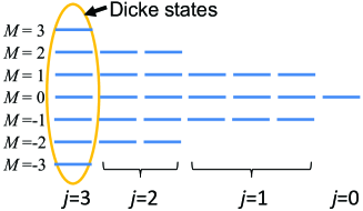
Figure 1: (color online). The energy level structure for $N=3$ three-level atoms ($j=1$). There are $(2j+1)^{3}=27$ levels, including the fully symmetric $2Nj+1=7$ states (the Dicke states).

To gain qualitative understanding of the Dicke superradiance, we start with considering an ensemble of ($2j+1$)-level atoms confined within a small region with its size much smaller than the wavelength of the radiation field. In this limit, the particles are indistinguishable viewed by the field and must be regarded as a whole quantum object. To emphasize that the collective radiative behavior is governed solely by many-body effects, we do not assume any instantaneous, i.e. non-radiative, interaction between atoms. The inter-particle spacing is large enough so that the overlap of particle wavepackets is negligible. In other words, the exchange interaction plays no role as well as the fermionic or bosonic nature of the atoms. Suppose that the transitions are induced by dipoles through the interaction Hamiltonian $V=-\sum_{i}\vec{p}_{i}\cdot\vec{E}(\vec{r}_{i})$, where $\vec{p}_{i}$ is the dipole operator of the $i$th atom and $\vec{E}(\vec{r}_{i})$ is the local field at the coordinate $\vec{r}_{i}$. Under the long-wavelength assumption of the field for a given small system size, the spatial dependence can be eliminated. Therefore $V=-\vec{E}\cdot\sum_{i}\vec{p}_{i}=-\sum_{\mu=x,y,z}\wp_{\mu}(E_{\mu}^{-}\hat{D}^{-}+\mbox{h.c.})$ in the rotating wave approximation. Here $\wp_{\mu}$ is the dipole moment magnitude of an atom in the $\mu$ direction, $E_{\mu}^{\pm}$ is the positive (negative) frequency component of the field, and $\hat{D}^{\pm}\equiv\sum_{i}\sigma_{i}^{\pm}$ with $\sigma_{i}^{-}\equiv\sum_{m=-J}^{J-1}|m\rangle_{i}\langle m+1|$ and $\sigma_{i}^{+}\equiv(\sigma_{i}^{-})^{\dagger}$. Note that $V$ does not break the permutational symmetry of the particles. If all the atoms are initially excited, time evolution will only take the state of the system around the fully symmetric manifold, whose eigenstates are usually called the Dicke states (See Fig. 1, PhysRev54_Dicke ; PhysRep82_Gross ):

$$|J,M\rangle=\sqrt{\frac{(J+M)!}{(2J)!(J-M)!}}(\hat{J}^{-})^{J-M}|J,J\rangle,$$ (1)

where $J=Nj$ is the total spin of $N$ spin-$j$ atoms and the integer $M$ denoting the level index can only go from $J$ through $-J$; the total spin ladder operators $\hat{J}^{\pm}=\sum_{i}\hat{j}_{i}^{\pm}$ satisfy $\hat{J}^{\pm}|J,M\rangle=\sqrt{J(J+1)-M(M\pm 1)}|J,M\pm 1\rangle$ with each $\hat{j}_{i}^{\pm}$ satisfying an analogous relation within the $i$th atom. The emission rate is then given by $W=\sum_{M}\rho_{M}W_{J}(M)$, where $\rho_{M}$ is the probability for the state being at the $M$th level, and the associated collective decay rate is $W_{J}(M)=\gamma\langle\hat{D}^{+}\hat{D}^{-}\rangle_{JM}$ with $\gamma$ denoting the bare rate in free space.

For spin-$\nicefrac{{1}}{{2}}$ particles, the ladder operator $\hat{j}_{i}^{\pm}$ happens to be, up to a constant factor, equivalent to the dipole operator, $\sigma_{i}^{-}=|g\rangle_{i}\langle e|$ and $\sigma_{i}^{+}=|e\rangle_{i}\langle g|$. This connection makes it straightforward to obtain $\langle\hat{D}^{+}\hat{D}^{-}\rangle_{JM}=(J+M)(J-M+1)$ PhysRep82_Gross . For spin-$j>\nicefrac{{1}}{{2}}$ atoms, the spin and dipole operators are no longer parallel. To obtain an explicit relation in this case, we take the mean-field assumption and get

$$\langle\hat{D}^{+}\hat{D}^{-}\rangle_{JM} = \sum_{i}\langle\sigma_{i}^{+}\sigma_{i}^{-}\rangle+\sum_{i\neq j}\langle\sigma_{i}^{+}\sigma_{j}^{-}\rangle$$ (2)

$$= N\langle\sigma_{1}^{+}\sigma_{1}^{-}\rangle_{JM}+N(N-1)\langle\sigma_{1}^{+}\sigma_{2}^{-}\rangle_{JM},$$

where $\langle\sigma_{1}^{+}\sigma_{1}^{-}\rangle_{JM}$ and $\langle\sigma_{1}^{+}\sigma_{2}^{-}\rangle_{JM}$ can be further expressed in terms of the Clebsch-Gordan coefficients:

$$\langle\sigma_{1}^{+}\sigma_{1}^{-}\rangle=1-\langle j,(N-1)j;-j,M+j|J,M\rangle^{2}$$ (3)

and

$$\langle\sigma_{1}^{+}\sigma_{2}^{-}\rangle = \sum_{m_{1},m_{2}}\Big{[}\langle j,(N-1)j;m_{1},M-m_{1}|J,M\rangle\langle j,(N-2)j;m_{2},M-m_{1}-m_{2}|J,M-m_{1}\rangle\times$$ (4)

$$\langle j,(N-1)j;m_{1}-1,M-m_{1}+1|J,M\rangle\langle j,(N-2)j;m_{2}+1,M-m_{1}-m_{2}|J,M-m_{1}+1\rangle\Big{]}.$$

The equation of motion now reads

$$\dot{\rho}_{M=J} = -W_{J}(J)\rho_{J},$$

$$\dot{\rho}_{M<J} = -W_{J}(M)\rho_{M}+W_{J}(M+1)\rho_{M+1}.$$ (5)

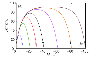
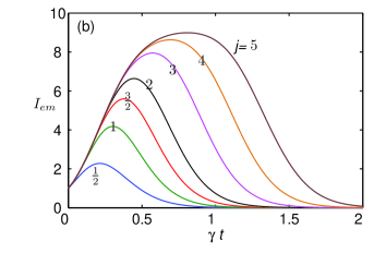
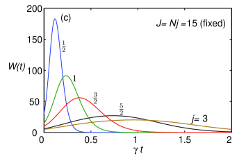
Figure 2: (color online). (a) $\langle\hat{D}^{+}\hat{D}^{-}\rangle_{JM}$ as a function of $M-J$ and (b) the emission intensity per particle $I_{\text{em}}$ of different spin $j$’s for $N=10$ atoms; (c) Overall emission curves for different spin $j$’s when $J=Nj=15$ is fixed. Note that $I_{\text{em}}$ and $W$ are in units of $\gamma\hbar\omega_{0}$ with the energy level spacing $\hbar\omega_{0}$.

The emission curves of different $j$ are shown in Fig. 2(b), for which we calculate the intensity per particle $I_{\text{em}}=W(t)/N$ with $N=10$ by evolving Eq. (5). One can observe that every curve shows a different degree of superradiance behavior, i.e., the intensity grows and maximizes in a short period of time. As $j$ increases, the peak intensity becomes higher. This implies that the radiation enhancement not only comes from many-body effects but also from multiple levels. This can be also seen in Fig. 2(a), where the enhancement factor $\langle\hat{D}^{+}\hat{D}^{-}\rangle_{JM}$ as a function of $M-J$ is plotted, consistently explaining the higher emission rate for larger $j$. One feature worth noting is that all $j$-curves in Fig. 2(b) share the same “growing” behavior. This is also suggested by the $\langle\hat{D}^{+}\hat{D}^{-}\rangle_{JM}$ curves in Fig. 2(a): For we start the radiation process from the fully excited state (the highest collective level), the dynamics is dominantly determined by the population flows associated with a few higher levels. The rates are proportional to the enhancement factor $\langle\hat{D}^{+}\hat{D}^{-}\rangle_{JM}$. For various $j$, we find in Fig. 2(a) that these curves coincide on the left hand side, corresponding to $|M-J|$ small (highest levels). Another noticeable feature is that the $\langle\hat{D}^{+}\hat{D}^{-}\rangle_{JM}$ curves develop a plateau as $j$ increases and the highest value is found to be bounded in the large-$j$ limit. It can then be expected that the peak intensity value should also have a bounded value for very large $j$. We will find this observation still true when we use a more sophisticated approach. More details will be discussed in Sec. III.

Finally, we compare the overall radiation by different spin-$j$ atoms, keeping the total spin $J=Nj$ fixed. Among these cases, they share the same $J$-Bloch sphere and therefore might be expected to have similar behaviors. However this is not true, as we can see from Fig. 2(c). Smaller $j$ cases have faster and more intense burst of emission while larger $j$ have smoother emission rates and longer tails. This is because $\langle\hat{D}^{+}\hat{D}^{-}\rangle_{JM}$, as determined by Eqs. (3) and (4), is also dependent on $N$, not merely dependent on the total spin $J$.

III Effective two-body formalism

We would like to emphasize that dipole-dipole interaction plays a crucial role and is responsible for both real and virtual photon exchange. As a consequence, the system builds up inter-particle coherence while decaying. As dipole-dipole interaction is contained in Dicke’s picture in a sense that the spin flip-flops count, this picture treats the whole system as a point-like object so that the inter-dipole coupling is considered uniform. In an actual laboratory setup, Dicke’s picture is usually an oversimplified view because a real sample always occupies a finite size and sees a finite wavelength of the radiative field. The spatial arrangement of particles usually breaks permutation symmetry. (Or more precisely, each particle sees different dipole-dipole couplings to all others.) The nonuniform coupling leads to dephasing of the Dicke states, resulting in population leakage out of the fully symmetric manifold. Furthermore, dipole-dipole interaction also causes other effects, e.g. frequency chirping, for which each Dicke state $|JM\rangle$ can be dipole-dipole shifted differently so that the emission frequency becomes variable over time PhysRep82_Gross . Superradiant behavior becomes more complex (and less pronounced) when these effects are not excluded. In order to better describe practical situations, we need to go over the microscopic details of atom-field interactions. The calculation, however, becomes intractable when the number of particles increases typically for $N\gtrsim 10$. In PRA99_Fleischhauer ; Yelin05 ; PRA07_Wang , we circumvent this difficulty by explicitly writing down the master equation of motion for only two probe atoms, taking average over the background atoms and tracing out the field variables. We also assume that the field instantaneously interacts with the whole ensemble, ignoring the retarding effects due to the finite size. (This can be justified because the characteristic time of propagation $d/c$ ($\sim 10^{-12}$ sec for a sample of size $d\sim 1$ mm) is usually much smaller than any other decay timescales.) We summarize here the main results and leave the details of the derivation to the Appendix. The relevant two-body master equation is given by

$$\dot{\rho} = -\sum_{i,j=1,2}\frac{\Gamma_{ij}}{2}\big{(}\big{[}\rho\sigma_{i}^{-},\sigma_{j}^{\dagger}\big{]}+\big{[}\sigma_{i}^{-},\sigma_{j}^{\dagger}\rho\big{]}\big{)}$$ (6)

$$- \sum_{i,j=1,2}\frac{\Gamma_{ij}+\gamma\delta_{ij}}{2}\big{(}\big{[}\rho\sigma_{j}^{\dagger},\sigma_{i}^{-}\big{]}+\big{[}\sigma_{j}^{\dagger},\sigma_{i}^{-}\rho\big{]}\big{)},$$

where $\rho$ is the two-body density matrix with dimension $(2j+1)^{2}\times(2j+1)^{2}$, $\gamma=\frac{\wp^{2}\omega_{0}^{3}}{3\pi\hbar\epsilon_{0}c^{3}}$ is the free-space spontaneous decay rate, $\Gamma\equiv\Gamma_{ii}$ is the single-particle induced pump/decay rate, and $\bar{\Gamma}\equiv\Gamma_{ij}$ ($i\neq j$) denotes the two-particle damping rate responsible for the atom-atom correlation. The mean-field approximation with the second order correction in fields gives the self-consistent form for the induced rate:

$$\Gamma = \gamma(e^{2\zeta}-1)\frac{A(t)}{V(t)}+2\mathcal{C}^{2}\varrho^{4}\frac{\gamma^{2}I(\zeta,\varrho)}{\Gamma+\gamma/2}Y(t)$$ (7)

$$\bar{\Gamma} = \frac{\gamma^{2}I(\zeta,\varrho)}{\Gamma+\gamma/2}\left[3\mathcal{C}\varrho A(t)+2\mathcal{C}^{2}\varrho^{4}Y(t)\right],$$ (8)

with

$$A(t) = \sum_{m=-j+1}^{j}\rho_{mm}^{(1)}$$ (9)

$$V(t) = \rho_{jj}^{(1)}-\rho_{-j,-j}^{(1)}$$ (10)

$$Y(t) = \sum_{m,m^{\prime}=-j}^{j-1}\rho_{m+1,m;m^{\prime},m^{\prime}+1},$$ (11)

where $\rho^{(1)}\equiv\frac{1}{2}\sum_{i=1,2}\text{tr}_{i}[\rho]$ denotes the reduced single-particle density matrix and $\rho_{ab;cd}\equiv\frac{1}{2}[\langle a,c||\rho|b,d\rangle+\langle c,a|\rho|d,b\rangle]$. The factor $\frac{1}{2}$ comes from averaging the interchanging of two particles. Note that interchange symmetry requires $\rho_{ab;cd}=\rho_{cd,ab}$ and $\rho_{ab;cd}^{\ast}=\rho_{ba;dc}$. The cooperativity parameter is defined as $\mathcal{C}\equiv 2\pi c^{3}\mathcal{N}/\omega^{3}$; $\varrho\equiv\omega d/(2c)$ characterizes the system size $d$ in terms of the radiation wavelength. These results are based on assumptions that there is no external field and hence the generated field has to be on-resonant with the transition frequency. Function $I(\zeta,\varrho)\equiv[\big{(}(\zeta-1)e^{\zeta}+\cos\varrho\big{)}^{2}+\big{(}\varrho e^{\zeta}-\sin\varrho\big{)}^{2}]/(\zeta^{2}+\varrho^{2})^{2}\approx\frac{e^{2\zeta}}{\zeta^{2}+\varrho^{2}}$ for large $\zeta$ and $\varrho$. If no thermal broadening is assumed, we have $\zeta\equiv\frac{1}{2}\mathcal{C}\varrho\frac{\gamma}{\Gamma+\gamma/2}V(t)$. When the Doppler broadening needs to be considered, the fields allow to be detuned and these quantities must be averaged. More details will be discussed in Sec. V.

IV Results

IV.1 Emission and decay rates

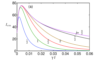
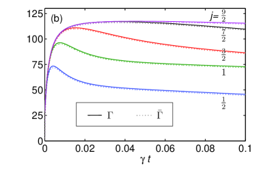
Figure 3: (color online). The temporal profiles of (a) the emission intensity per particle (in units of $\gamma\hbar\omega_{0}$) and (b) the induced single-atom pump/decay rate $\Gamma$ and two-atom correlation damping rate $\bar{\Gamma}$ (in units of $\gamma$). In all cases we use $\mathcal{C}=10$ and $\varrho=10$.

By Eq. (6) we are able to solve for the temporal emission rate curve. Fig. 3(a) shows the radiation intensity per particle $I_{\text{em}}$ with $\mathcal{C}=10$ and $\varrho=10$ for different spin-$j$ species, where $I_{\text{em}}\equiv\hbar\omega_{0}\sum_{m=-j}^{j}(j+m)\frac{d}{dt}\rho_{mm}^{(1)}(t)$. Here we take $\rho_{jj,jj}=1$ and set $0$ for all other density matrix elements as the initial state. It can be seen that for each $j$ the radiation intensity reaches a peak, giving a strong evidence of superradiance. Those curves follow roughly the same intensity profile in the beginning. The maximal value of intensity first grows as $j$ increases from $\nicefrac{{1}}{{2}}$, and then stops growing when $j\gtrsim 2$. The time of reaching the peak intensity also converges to a fixed constant $t_{\text{max}}$ in the large $j$ limit. This also has been observed in the Dicke superradiance picture. Here we give an intuitive explanation as follows: When the system starts to relax from the state with all atoms initially excited to the highest level, only a few highest levels are involved in determining the radiative behavior during the early stage. Even for a very large spin particle, who has a huge multi-level structure, those levels lower than the first few have not been populated yet and hence do not have contributions. The time evolution of the decay rates is also plotted in Fig. 3(b). Note that at $t=0$ the diagonal decay rate $\Gamma(0)$ determines the initial emission intensity, followed by a sharp growth and hence resulting in intensity peaks. In the mean time, the off-diagonal $\bar{\Gamma}$ emerges and mixes single-body states. Different from the Dicke picture, where we choose the eigenbasis to be the symmetric states constructed by a giant spin object $J=Nj$, here we use products of single particle states as the eigenbasis, allowing the degrees of freedom of population being transferred to asymmetric levels. Note that the dipole-dipole interaction is built-in in our formalism and is responsible for these effects. Consequently, the superradiance enhancement with $j$, when characterized by the growth of peak intensity, in more realistic cases cannot be as large as predicted by the Dicke model. On the other hand, since the asymmetric levels have lower or vanishing decay rates, the occupation of these levels modifies the tails of the emission curves. In some circumstances, the energy is trapped. Such effects cannot be described by the Dicke model.

A few remarks are placed here regarding the connection of cooperativity and superradiant curves. As we increase $\mathcal{C}$ ($\varrho$) while fixing $\varrho$ ($\mathcal{C}$), the emission peak intensity per particle increases proportionally while the time scale of the initial intensity burst is inversely proportional to $\mathcal{C}$ ($\varrho$). This is due to the “many-body enhancement”, as we have discussed using Dicke’s picture. Such features are commonly observed even in the original two-level systems. Furthermore, the emission curves are found to be similar when $\mathcal{C}\varrho$ is kept the same (not shown). This can also be seen analytically (see Appendix). This suggests that $\mathcal{C}\varrho\sim\mathcal{N}\lambda^{2}d$ be the relevant factor that determines the primary superradiant behavior while the detailed emission curves, however, still slightly depend on $\mathcal{C}$ and $\varrho$ separately PRL08_Akkermans ; PRA07_Wang .

IV.2 Significance of atom-atom coherence

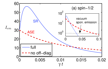
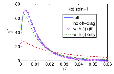
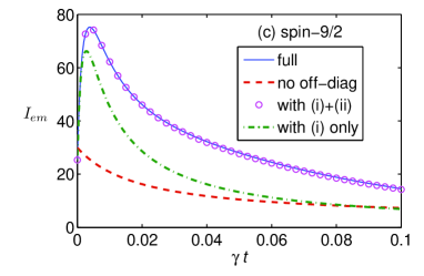
Figure 4: (color online). Evolution curves for emission intensity when the off-diagonal terms are fully considered (full), partially removed (with both (i) and (ii), or only with (i); see text), or entirely removed (no off-diag) for (a) spin-$\nicefrac{{1}}{{2}}$, (b) spin-$1$, and (c) spin-$\nicefrac{{9}}{{2}}$ particles. Other parameters are the same as Fig. 3. Inset of (a): We plot three curves of superradiance (SR, blue solid), amplified spontaneous emission (ASE, red dashed), and single-particle free-space spontaneous emission (black dotted) for comparison.

Cooperation of many-body states is crucial to superradiance. The beauty of this formalism is that we retain the accessibility to atom-atom correlations under the framework of the mean field approximation. Here we investigate the role of many-body correlations, which, in our case, are contained in the off-diagonal terms of the two-body density matrix. To see this, this method allows us to manipulate these off-diagonal terms and evolve Eq. (6). The results will then be compared. Note that these off-diagonal terms have the form $\rho_{a,a+m;b,b-m}$. In the spin-$\nicefrac{{1}}{{2}}$ case, the only possibility is $\rho_{eg,ge}$. Fig. 4(a) shows the emission curve for $\mathcal{C}=10$, $\varrho=10$, and $\rho_{eg,ge}=0$ at all time. This curve is now found to be monotonically descending, signaling mere amplified spontaneous emission (ASE) instead of superradiance (SR) because of apparent lack of an intensity peak. Such monotonicity is shared by larger $j$ cases (Figs. 4(b) and (c)) when all off-diagonal terms are set to zero. The reason is clear: Without atom-atom correlation, the density matrix is reduced to a single-particle description and therefore no cooperative effects are observed. On the other hand, for larger $j$ atoms the off-diagonal terms does not only concern atom-atom correlations from the same-level transitions but also involve that from different-level density matrix elements. In the following we try to distinguish the importance from three kinds of coherence terms: (i) the same-level coherence $\rho_{a,a+1;a+1,a}$, (ii) the cross-coherence $\rho_{a,a+1;b+1,b}$ for $a\neq b$, and (iii) the higher-order coherence $\rho_{a,a+m;b,b-m}$ for $m\geq 2$. For example, in Figs. 4(b) for spin-$1$ and (c) for spin-$\nicefrac{{9}}{{2}}$ atoms, we plot the emission curves corresponding to all off-diagonal terms being dropped out, and (i), (ii), and then (iii) being added back to the system. It can be found that by inclusion of (i) and (ii) the system has already behaved like the actual dynamics, indicating that the higher-order coherence is negligible in determining the evolution of the system. However, if only (i) is included, although the intensity enhancement can still be observed, the details of emission profile have discrepancy to the actual behaviors. The distinction becomes even more obvious when $j$ gets large, as we see in Fig. 4(c). The fact that the cross-coherence terms must be taken into consideration implies the interferences due to “cross-level” transitions, i.e., the transitions of the same energy difference, but not from two definite levels, have some kind of “multi-level” contributions to the superradiance, in analog to the many-body effects.

V Doppler broadening

When a hot gas is considered, the energy difference seen by moving atoms varies. In this section we consider the loss of coherence due to the Doppler effects. Suppose that the thermal gas is described by a Gaussian distribution function:

$$f_{D}(\delta)=\frac{1}{\sqrt{2\pi}\Delta_{D}}\exp\Big{[}-\frac{\delta^{2}}{2\Delta_{D}^{2}}\Big{]},$$ (12)

where $\delta$ is the Doppler shift for an atom and $\Delta_{D}$ is the characteristic width of this distribution. In order to take this average into account we need to go to the derivation summarized in the Appendix. Note that the frequency difference between the field and the Fourier component $\Delta$ in Eqs. (40,41) is now modified to $\Delta-\delta$. Here we also assume that the velocity distribution will not be affected by atoms’ recoil when photons are emitted. The idea is then to divide the whole system in the frequency space into a series of small slivers according to the detunings they see individually. For each sliver, it can be expected that the integration as in Eqs. (40,41) should lead to the same spatial dependence. The only modification is that the source and retarded functions (43,44,42) and Green’s functions (45) need to be determined in an averaged manner because they contain the effects from all slivers. For convenience we use a notation that $\bar{Q}=\int_{-\infty}^{\infty}Q(\delta)f_{D}(\delta)d\delta$ to represent an Doppler averaged quantity. Consequently,

$$\overline{\widetilde{P}^{ret}}(\Delta) = \frac{\mathcal{N}\wp^{2}}{\hbar^{2}}V(t)\overline{\frac{1}{\Gamma_{f}-i(\Delta-\delta)}}$$ (13)

$$= \frac{\mathcal{N}\wp^{2}}{\hbar^{2}}\frac{V(t)}{\Delta_{D}}\sqrt{\frac{\pi}{2}}U(iz_{0}),$$

$$\overline{\widetilde{P}^{s}}(\Delta) = \frac{\mathcal{N}\wp^{2}}{\hbar^{2}}\frac{2A(t)}{\Delta_{D}}\sqrt{\frac{\pi}{2}}\mbox{Re}[U(iz_{0})]$$ (14)

$$\overline{\widetilde{D}^{ret}}(\vec{x},\Delta) = -\frac{i\hbar\omega^{2}}{6\pi\epsilon_{0}c^{2}}\frac{e^{\overline{q_{0}^{\prime\prime}}x}}{x}e^{-i\overline{q_{0}^{\prime}}x},$$ (15)

where $U(z)\equiv\frac{2}{\sqrt{\pi}}\int_{z}^{\infty}e^{z^{2}-s^{2}}ds$ is the scaled complementary error function and $z_{0}=\frac{\Gamma+\gamma/2+i\Delta}{\sqrt{2}\Delta_{D}}$; $\overline{q_{0}^{\prime\prime}}=\frac{C\gamma\varrho}{d}V(t)\frac{1}{\Delta_{D}}\sqrt{\frac{\pi}{2}}U(iz_{0})$ while $\overline{q_{0}^{\prime}}=q_{0}=\omega/c$ keeps the same. Finally we have

$$\Gamma(\Delta) = \gamma(e^{2\bar{\zeta}}-1)\frac{A(t)}{V(t)}$$ (16)

$$+2\frac{\gamma^{2}}{\Delta_{D}}\mathcal{C}^{2}\varrho^{4}I(\bar{\zeta},\bar{\varrho})\mbox{Re}[U(iz_{0})]Y(t)$$

$$\bar{\Gamma}(\Delta) = \frac{\gamma^{2}}{\Delta_{D}}I(\bar{\zeta},\bar{\varrho})\mbox{Re}[U(iz_{0})]\times$$ (17)

$$\left[3\mathcal{C}\varrho A(t)+2\mathcal{C}^{2}\varrho^{4}Y(t)\right],$$

where

$$\bar{\varrho}(\Delta) = \varrho+\frac{1}{2}\sqrt{\frac{\pi}{2}}\mathcal{C}\gamma\varrho\frac{V(t)}{\Delta_{D}}\text{Re}[U(iz_{0})]$$ (18)

$$\bar{\zeta}(\Delta) = \frac{1}{2}\sqrt{\frac{\pi}{2}}\mathcal{C}\gamma\varrho\frac{V(t)}{\Delta_{D}}\text{Im}[U(iz_{0})].$$ (19)

Each sliver, depending on its location at the thermal distribution function, sees these quantities associated with a specific Fourier component $\Delta$. The overall decay is then equivalent to averaging $\Gamma$ and $\bar{\Gamma}$ according to the thermal distribution function, i.e.,

$$\Gamma_{ij}^{D}=\int_{-\infty}^{\infty}d\Delta\frac{1}{\sqrt{2\pi}\Delta_{D}}e^{-\Delta^{2}/(2\Delta_{D}^{2})}\Gamma_{ij}(\Delta).$$ (20)

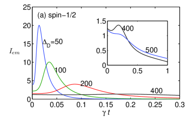
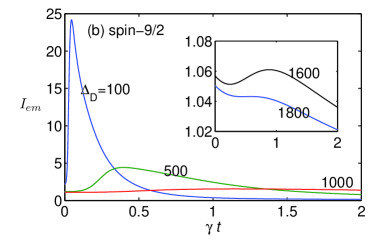
Figure 5: (color online). Doppler-broadened emission intensity curves for (a) spin-$\nicefrac{{1}}{{2}}$ and (b) spin-$\nicefrac{{9}}{{2}}$ particles. The inset figures show, for each case, two curves slightly smaller and larger than the marginal Doppler width $\Delta_{m}$. Here we use $\mathcal{C}=10$ and $\varrho=10$ for both cases, and get (a) $\Delta_{m}/\gamma=433$ and (b) $\Delta_{m}/\gamma=1650$.

Eq. (20) is solved numerically. We then calculate the corresponding emission curves and show them in Fig. 5. With the Doppler broadening, it is clear that the superradiance behavior is suppressed as the Doppler width $\Delta_{D}$ increases. This is due to frequency mismatch and therefore part of the atoms loses track of coherence and decays more independently. But the superradiance peaks are still observable within a certain range of $\Delta_{D}$, until it becomes too large and kills the peaks. This is understandable because for a small-width distribution, there are still sufficient atoms located within a frequency-matching regime. In order to characterize the existence of superradiance when the match and mismatch parts compete, we define a marginal Doppler width $\Delta_{m}$ beyond which the peak value no longer surpasses the initial intensity. Obviously $\Delta_{m}$ depends on the cooperativity parameter $\mathcal{C}$, and in Figs. 6(a) and (b) we plot the relations for spin-$\nicefrac{{1}}{{2}}$ and spin-$\nicefrac{{9}}{{2}}$ particles, respectively. We find approximately a quadratic dependence $\Delta_{m}\propto\mathcal{C}^{2}$. Note that when the cooperativity parameter increases, not only the total number of particle increases but the inter-particle spacing decreases accordingly. This enhances the dipole-dipole interaction (of the order of magnitude $\wp^{2}/(2\pi\epsilon_{0}r^{3})\propto\mathcal{C}$) which is responsible for the superradiance for an additional factor $\mathcal{C}$. As a result we have the tolerance $\Delta_{m}$ with a quadratic dependence on $\mathcal{C}$ rather than a linear dependence.

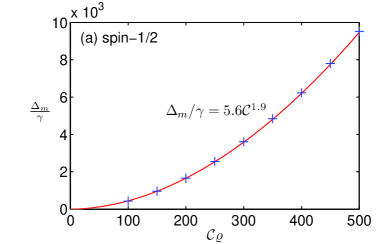
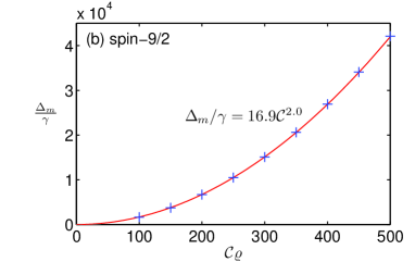
Figure 6: (color online). The marginal Doppler width $\Delta_{m}$ as a function of the cooperativity for (a) spin-$\nicefrac{{1}}{{2}}$ and (b) spin-$\nicefrac{{9}}{{2}}$ particles. (Here we take $\varrho=10$). The cross dots (blue) represent our calculated data; the solid lines (red) are best fitting power-law curves with the exponent around $2$.

VI Molecular vibrational states

One direct example for multi-level structure is vibrational modes of polar molecules where the deeply bound potential can be well approximated by a harmonic one. The number of low lying eigenstates that are quasi-equally spaced energy levels can usually be up to a few tens. These particles are thus analogous to large “spin” particles. Take a typical example of heteronuclear diatomic alkali molecules Deiglmayr11 : the state $X^{1}\Sigma^{+}$ for LiCs has an averaged energy spacing $\omega_{0}\approx 2\pi\times 5$ THz. For a sample of LiCs molecules with a density $\mathcal{N}\approx 4\times 10^{9}$ $\mbox{cm}^{-3}$, such energy spacing corresponds to cooperativity $\mathcal{C}\sim 20\gg 1$. The transitional dipole moment between two adjacent vibrational states is about $5$ Debye, and therefore the single-particle spontaneous emission rate $\gamma\sim\mbox{sec}^{-1}$. We then expect within this parameter regime that superradiance intensity peak can be observed in a timescale of mini-sec while $\Gamma_{\text{max}}\gtrsim 1000\gamma$.

The cascade relaxation of excited population from higher to lower levels is a reminiscence of motional cooling. When the cooperative effect comes into play, the down-ladder process will be accelerated because the stimulated decay becomes dominant while superradiance takes place (without other pumping processes such as thermal excitation). As we have pointed out, the induced rate can be a few orders of magnitude by increasing the number of particles and hence the cooperativity. This suggests a scheme of “superradiance-assisted cooling”. Such scheme may be an alternative to cool vibrational states of molecules, which, generally speaking, has previously been obstructed by the fact that such states are only weakly optically coupled.

APPENDIX

VI.1 Two-body master equation

Figure 7: Schwinger-Keldysh contour

Although this method of the effective two-body description has been discussed in great details in PRA99_Fleischhauer ; Yelin05 , we summarize in this section the derivation for the formalism for completeness. We start with the microscopic Hamiltonian that reads

$$H = \underbrace{H_{\text{atom}}+H_{\text{field}}-\sum_{j\notin\{1,2\}}\vec{p}_{j}\cdot(\vec{\mathcal{E}}(\vec{r}_{i},t)+\vec{E}(\vec{r}_{j},t))}_{H_{0}}$$ (21)

$$-\underbrace{\sum_{i=1}^{2}\vec{p}_{i}\cdot(\vec{\mathcal{E}}(\vec{r}_{i},t)+\vec{E}(\vec{r}_{i},t))}_{V}.$$

Here, we separate the field into two parts: the external classical driving field $\vec{\mathcal{E}}(\vec{r}_{i},t)$ and the induced local field $\vec{E}(\vec{r}_{i},t)$. When a uniform dense gas of atoms is considered, it is reasonable to assume that every atom sees the same field and the same background due to other atoms. On the other hand, in order to take into account atom-atom quantum correlation we need to retain adequate degrees of freedom involving at least two particles. Our proposal is therefore to write down an effective description for two probe atoms in which all other atoms’ contribution will be averaged in the mean-field sense and appear as parameters in the two-body description. In Eq. (21) $V$ is the interaction of the probe atoms ($i=1$, $2$) with the field and will be treated as a small perturbation. $H_{0}$ consists of the unperturbed atomic and field Hamiltonian as well as the contribution from the background atoms. In the interaction picture, the evolution operator is then given by

$$S_{I}(t)=T\exp\Big{[}-\frac{i}{\hbar}\int_{-\infty}^{t}V_{I}(t^{\prime})dt^{\prime}\Big{]},$$ (22)

where $T$ is the time-ordering operator. We here introduce the positive and negative components $x(t)=x^{+}(t)+x^{-}(t)$ with $x^{\pm}(t)=\widetilde{x}(t)e^{\mp i\omega t}$, where $x_{\mu}\in\{p_{i\mu},E_{\mu},\mathcal{E}_{\mu}\}$ and $\widetilde{x}(t)$ is the slowly varying (compared to the inverse of the radiation frequency $\omega^{-1}$) amplitude of the corresponding quantity. Further note that $\widetilde{p}_{i\mu}^{+}=\wp_{\mu}\sigma_{i}^{-}$ and $\widetilde{p}_{i\mu}^{-}=\wp_{\mu}\sigma_{i}^{+}$. In the rotating wave approximation, the interaction becomes $V_{I}(t)\simeq\sum_{i\mu}[p_{i\mu}^{+}(E_{\mu}^{-}+\mathcal{E}_{\mu}^{-})+\mbox{h.c.}]$. Eq. (22) can be cast in the framework of Schwinger-Keldysh formalism, in which $V_{I}(t)\longrightarrow V(\check{\tau})$ and $S_{I}(t)\longrightarrow$

$$S_{C}=T_{C}\exp\Big{[}-\frac{i}{\hbar}\int_{C}V(\check{\tau})d\check{\tau}\Big{]},$$ (23)

where $C$ denotes the Schwinger-Keldysh contour as shown in Fig. 7, and $T_{C}$ is the contour-oriented time-ordering operator, i.e., along the upper branch of the contour $T_{C}$ is the normal time-ordering operator while along the lower branch is the inverse time-ordering operator. To prevent possible confusion we denote the “time” parameter along the Keldysh contour with a check sign. We then trace out the degrees of freedom of the fields and the background atoms, which leads to an effective evolution operator:

$$S_{C}^{\text{eff}}=\langle S_{C}\rangle_{\text{field}}$$

$$=T_{C}\exp\bigg{\{}\frac{i}{\hbar}\int_{C}d\check{\tau}\sum_{i=1}^{2}\sum_{\mu}\Big{[}p_{i\mu}^{+}(\check{\tau})\mathcal{E}_{L\mu}^{-}(\vec{r}_{i},\check{\tau})$$

$$+p_{i\mu}^{-}(\check{\tau})\mathcal{E}_{L\mu}^{+}(\vec{r}_{i},\check{\tau})\Big{]}$$ (24)

$$-\frac{1}{2\hbar^{2}}\iint_{C}d\check{\tau}_{1}d\check{\tau}_{2}\sum_{i,j=1}^{2}\sum_{\mu\nu}\Big{[}p_{i\mu}^{+}(\check{\tau}_{1})D_{i\mu,j\nu}(\check{\tau}_{1},\check{\tau}_{2})p_{j\nu}^{-}(\check{\tau}_{2})$$

$$+p_{i\mu}^{-}(\check{\tau}_{1})C_{i\mu,j\nu}(\check{\tau}_{1},\check{\tau}_{2})p_{j\nu}^{+}(\check{\tau}_{2})\Big{]}\bigg{\}},$$

where $\vec{\mathcal{E}}_{L}^{\pm}(\vec{r}_{i},\check{\tau})=\vec{\mathcal{E}}^{\pm}(\vec{r}_{i},\check{\tau})+\langle\vec{E}^{\pm}(\vec{r}_{i},\check{\tau})\rangle$ is the local field seen by the probe atom, and the Green’s function of the interacting field

$$D_{i\mu,j\nu}(\check{\tau}_{1},\check{\tau}_{2}) = \langle\!\langle T_{C}E_{\mu}^{-}(\vec{r}_{i},\check{\tau}_{1})E_{\nu}^{+}(\vec{r}_{j},\check{\tau}_{2})\rangle\!\rangle$$ (25)

$$C_{i\mu,j\nu}(\check{\tau}_{1},\check{\tau}_{2}) = \langle\!\langle T_{C}E_{\mu}^{+}(\vec{r}_{i},\check{\tau}_{1})E_{\nu}^{-}(\vec{r}_{j},\check{\tau}_{2})\rangle\!\rangle.$$ (26)

To get Eq. (24) we have used

$$\big{<}T_{C}\exp[s\hat{A}]\big{>} = \exp\bigg{[}\sum_{m}\frac{s^{m}}{m!}\langle\!\langle T_{C}\hat{A}^{m}\rangle\!\rangle\bigg{]},$$ (27)

with $\langle\!\langle\cdot\rangle\!\rangle$ denoting the cumulant, which is defined by

$$\langle\!\langle\hat{A}\rangle\!\rangle = \langle\hat{A}\rangle$$

$$\langle\!\langle\hat{A}\hat{B}\rangle\!\rangle = \langle\hat{A}\hat{B}\rangle-\langle\hat{A}\rangle\langle\hat{B}\rangle,$$

where $\hat{A}$ and $\hat{B}$ are operators. We also set the higher-order cumulants $\langle\!\langle E^{m}\rangle\!\rangle=0$ for $m>2$ by assuming that the radiation field is Gaussian. The two-field Green’s function $D_{i\mu,j\nu}(\check{\tau}_{1},\check{\tau}_{2})$, depending on the order of $\check{\tau}_{1}$ and $\check{\tau}_{2}$ on $C$, has four possible forms:

$$D_{\mu\nu}^{++} = \langle\!\langle TE_{\mu}^{-}(\vec{r}_{i},\tau_{1+})E_{\nu}^{+}(\vec{r}_{j},\tau_{2+})\rangle\!\rangle$$ (28)

$$D_{\mu\nu}^{--} = \langle\!\langle T^{-1}E_{\mu}^{-}(\vec{r}_{i},\tau_{1-})E_{\nu}^{+}(\vec{r}_{j},\tau_{2-})\rangle\!\rangle$$ (29)

$$D_{\mu\nu}^{-+} = \langle\!\langle E_{\mu}^{-}(\vec{r}_{i},\tau_{1-})E_{\nu}^{+}(\vec{r}_{j},\tau_{2+})\rangle\!\rangle$$ (30)

$$D_{\mu\nu}^{+-} = \langle\!\langle E_{\nu}^{+}(\vec{r}_{j},\tau_{2-})E_{\mu}^{-}(\vec{r}_{i},\tau_{1+})\rangle\!\rangle.$$ (31)

The other Green’s function $C_{i\mu,j\nu}$ has similar relations. By the subscript “+” or “-” we denote the upper or lower branch for $\tau$, respectively. In Eq. (24), those terms like

$$\iint_{C}d\check{\tau}_{1}d\check{\tau}_{2}p_{i\mu}^{+}(\check{\tau}_{1})D_{i\mu,j\nu}(\check{\tau}_{1},\check{\tau}_{2})p_{j\nu}^{-}(\check{\tau}_{2})$$

$$=\sum_{A,B\in\{+,-\}}\kappa_{AB}\wp_{\mu}\wp_{\nu}\int_{-\infty}^{\infty}d\tau_{1}\int_{-\infty}^{\infty}d\tau_{2}\times$$ (32)

$$\qquad\qquad\sigma_{iA}^{-}D_{i\mu,j\nu}^{AB}(\tau_{1},\tau_{2})\sigma_{jB}^{+}e^{i\omega(\tau_{2}-\tau_{1})},$$

where $\kappa_{AB}=1$ for $A=B$ and $\kappa_{AB}=-1$ for $A\neq B$, and the subscripts $A,B$ being placed with $\sigma^{-}$ and $\sigma^{+}$ emphasizes that the operators must be in order accordingly on the Schwinger-Keldysh contour $C$. We change the time variables for the field correlation such that $D_{i\mu,j\nu}^{AB}(\tau_{1},\tau_{2})\longrightarrow D_{i\mu,j\nu}^{AB}(\tau,\tau^{\prime})$ with $\tau_{1}=\tau-\tau^{\prime}/2$ and $\tau_{2}=\tau+\tau^{\prime}/2$. After some math, we reach

$$S_{C}^{\text{eff}} = T_{c}\exp\bigg{\{}\sum_{i,\mu}\frac{i\wp_{\mu}}{\hbar}\int_{-\infty}^{\infty}d\tau\big{[}\sigma_{i}^{-}(\tau_{+})\mathcal{E}_{L\mu}^{-}(\vec{r}_{i},\tau)-\sigma_{i}^{-}(\tau_{-})\mathcal{E}_{L\mu}^{-}(\vec{r}_{i},\tau)+\sigma_{i}^{+}(\tau_{+})\mathcal{E}_{L\mu}^{+}(\vec{r}_{i},\tau)-\sigma_{i}^{+}(\tau_{-})\mathcal{E}_{L\mu}^{+}(\vec{r}_{i},\tau)\big{]}$$ (33)

$$-\int_{-\infty}^{\infty}d\tau\frac{\Gamma_{i\mu,j\nu}(\omega,\tau)}{2}\big{[}\sigma_{i}^{-}(\tau_{+})\sigma_{j}^{+}(\tau_{+})+\sigma_{i}^{-}(\tau_{-})\sigma_{j}^{+}(\tau_{-})-2\sigma_{i}^{-}(\tau_{-})\sigma_{j}^{+}(\tau_{+})\big{]}$$

$$-\int_{-\infty}^{\infty}d\tau\frac{\Gamma_{i\mu,j\nu}(\omega,\tau)+\gamma_{i\mu,j\nu}(\omega,\tau)}{2}\big{[}\sigma_{j}^{+}(\tau_{+})\sigma_{i}^{-}(\tau_{+})+\sigma_{j}^{+}(\tau_{-})\sigma_{i}^{-}(\tau_{-})-2\sigma_{j}^{+}(\tau_{-})\sigma_{i}^{-}(\tau_{+})\big{]}$$

$$+\frac{i}{\hbar}\int_{-\infty}^{\infty}d\tau H_{i\mu,j\nu}(\omega,\tau)\big{[}\sigma_{i}^{-}(\tau_{+})\sigma_{j}^{+}(\tau_{+})-\sigma_{i}^{-}(\tau_{-})\sigma_{j}^{+}(\tau_{-})-\sigma_{j}^{+}(\tau_{+})\sigma_{i}^{-}(\tau_{+})+\sigma_{j}^{+}(\tau_{-})\sigma_{i}^{-}(\tau_{-})\big{]}$$

$$+\frac{i}{\hbar}\int_{-\infty}^{\infty}d\tau h_{i\mu,j\nu}(\omega,\tau)\big{[}\sigma_{j}^{+}(\tau_{+})\sigma_{i}^{-}(\tau_{+})+\sigma_{j}^{+}(\tau_{-})\sigma_{i}^{-}(\tau_{-})\big{]}\bigg{\}},$$

where we have introduced these quantities:

$$\Gamma_{i\mu,j\nu}(\tau,\omega) = \frac{\wp_{\mu}\wp_{\nu}}{\hbar^{2}}\int_{-\infty}^{\infty}d\tau^{\prime}\langle\!\langle E_{\mu}^{-}(\vec{r}_{i},\tau)E_{\nu}^{+}(\vec{r}_{j},\tau+\tau^{\prime})\rangle\!\rangle e^{i\omega\tau^{\prime}},$$ (34)

$$\gamma_{i\mu,j\nu}(\tau,\omega) = \frac{\wp_{\mu}\wp_{\nu}}{\hbar^{2}}\int_{-\infty}^{\infty}d\tau^{\prime}\langle\big{[}E_{\mu}^{+}(\vec{r}_{i},\tau),E_{\nu}^{-}(\vec{r}_{j},\tau+\tau^{\prime})\big{]}\rangle e^{i\omega\tau^{\prime}},$$ (35)

$$H_{i\mu,j\nu}(\tau,\omega) = \frac{i\wp_{\mu}\wp_{\nu}}{2\hbar}\int_{0}^{\infty}d\tau^{\prime}\big{\{}\langle\!\langle E_{\mu}^{-}(\vec{r}_{i},\tau)E_{\nu}^{+}(\vec{r}_{j},\tau-\tau^{\prime})\rangle\!\rangle e^{-i\omega\tau^{\prime}}-\langle\!\langle E_{\mu}^{-}(\vec{r}_{i},\tau)E_{\nu}^{+}(\vec{r}_{j},\tau+\tau^{\prime})\rangle\!\rangle e^{i\omega\tau^{\prime}}\big{\}},$$ (36)

$$h_{i\mu,j\nu}(\tau,\omega) = \frac{i\wp_{\mu}\wp_{\nu}}{2\hbar}\int_{0}^{\infty}d\tau^{\prime}\big{\{}\langle\big{[}E_{\mu}^{-}(\vec{r}_{i},\tau),E_{\nu}^{+}(\vec{r}_{j},\tau-\tau^{\prime})\big{]}\rangle e^{-i\omega\tau^{\prime}}-\langle\big{[}E_{\mu}^{-}(\vec{r}_{i},\tau),E_{\nu}^{+}(\vec{r}_{j},\tau+\tau^{\prime})\big{]}\rangle e^{i\omega\tau^{\prime}}\big{\}}.$$ (37)

From Eq. (33) we extract the effective master equation:

$$\dot{\rho}(t)=-\frac{i}{\hbar}\big{[}H_{0},\rho\big{]}$$

$$+\sum_{j=1,2}\sum_{\mu}\frac{i}{\hbar}\wp_{\mu}\big{[}\sigma_{j}^{-}\mathcal{E}_{L,\mu}^{-}(\vec{r}_{j})+\sigma_{j}^{\dagger}\mathcal{E}_{L,\mu}^{+}(\vec{r}_{j}),\rho\big{]}$$

$$+\frac{i}{\hbar}\sum_{i=1,2}\sum_{\mu,\nu}H_{i\mu,i\nu}\Big{[}\big{[}\sigma_{i\mu}^{-},\sigma_{i\nu}^{+}\big{]},\rho\Big{]}$$ (38)

$$-\sum_{i,j=1,2}\sum_{\mu,\nu}\frac{\Gamma_{i\mu,j\nu}}{2}\big{(}\big{[}\rho\sigma_{i}^{-},\sigma_{j}^{\dagger}\big{]}+\big{[}\sigma_{i}^{-},\sigma_{j}^{\dagger}\rho\big{]}\big{)}$$

$$-\sum_{i,j=1,2}\sum_{\mu,\nu}\frac{\Gamma_{i\mu,j\nu}+\gamma_{i\mu,j\nu}}{2}\big{(}\big{[}\rho\sigma_{j}^{\dagger},\sigma_{i}^{-}\big{]}+\big{[}\sigma_{j}^{\dagger},\sigma_{i}^{-}\rho\big{]}\big{)}.$$

Note that $\rho$ is the two-body density operator so is a $(2j+1)^{2}\times(2j+1)^{2}$ matrix. Now we identify term $\Gamma$ as the induced pump and decay rate and term $\gamma$ as the spontaneous decay rate inside the atomic medium. Term $h$ as shown in Eq. (37) corresponds to the Lamb shifts, which are somewhat irrelevant for our current consideration and is therefore absorbed to the unperturbed Hamiltonian $H_{0}$; term $H$ as shown in Eq. (36) accounts for the collective light shifts and inhomogeneous broadening. In this paper, we neglect the dipole shifts and frequency chirping by dropping the diagonal shift terms, and stress on the quantum correction that makes significance to the superradiance mechanism. The relevant part of the master equation now reads

$$\dot{\rho} = -\sum_{i,j=1,2}\frac{\Gamma_{ij}}{2}\big{(}\big{[}\rho\sigma_{i}^{-},\sigma_{j}^{\dagger}\big{]}+\big{[}\sigma_{i}^{-},\sigma_{j}^{\dagger}\rho\big{]}\big{)}$$ (39)

$$- \sum_{i,j=1,2}\frac{\Gamma_{ij}+\gamma\delta_{ij}}{2}\big{(}\big{[}\rho\sigma_{j}^{\dagger},\sigma_{i}^{-}\big{]}+\big{[}\sigma_{j}^{\dagger},\sigma_{i}^{-}\rho\big{]}\big{)}.$$

We follow the derivation in PRA99_Fleischhauer ; Yelin05 and summarize the main results. $\Gamma_{ij}$ can be evaluated through

$$\Gamma = \frac{\wp^{2}}{\hbar^{2}}\int d^{3}x\left|\widetilde{D}^{ret}(\vec{r}_{0},t|\vec{x},\Delta)\right|^{2}\widetilde{P}^{(1)s}(\vec{r}_{0},t|\Delta)$$ (40)

$$+ \frac{\wp^{2}}{\hbar^{2}}\int\int d^{3}x_{1}d^{3}x_{2}\widetilde{D}^{ret}(\vec{r}_{0},t|\vec{x}_{1},\Delta)\widetilde{D}^{\ast ret}(\vec{r}_{0},t|\vec{x}_{2},\Delta)\widetilde{P}^{(2)s}(\vec{r}_{0},t|\vec{x}_{1},\vec{x}_{2},\Delta)$$

$$\bar{\Gamma} = \frac{\wp^{2}}{\hbar^{2}}\int d^{3}x\widetilde{D}^{ret}(\vec{r}_{0},t|\vec{x},\Delta)\widetilde{D}^{\ast ret}(\vec{r}_{0},t|\vec{x},\Delta)\widetilde{P}^{(1)s}(\vec{r}_{0},t|\Delta)$$ (41)

$$+ \frac{\wp^{2}}{\hbar^{2}}\int\int d^{3}x_{1}d^{3}x_{2}\widetilde{D}^{ret}(\vec{r}_{0},t|\vec{x}_{1},\Delta)\widetilde{D}^{\ast ret}(\vec{r}_{0},t|\vec{x}_{2},\Delta)\widetilde{P}^{(2)s}(\vec{r}_{0},t|\vec{x}_{1},\vec{x}_{2},\Delta).$$

We denote $\Gamma\equiv\Gamma_{ii}$ and $\bar{\Gamma}\equiv\Gamma_{ij}$ for $i\neq j$. For above, the retarded function $\widetilde{P}^{ret}$, the single-particle and two-particle source functions $\widetilde{P}^{(1)s}$ and $\widetilde{P}^{(2)s}$ are given respectively by

$$\widetilde{P}^{ret}(\vec{r}_{0},t|\Delta) = \frac{\mathcal{N}\wp^{2}}{\hbar^{2}}\left[\frac{V(t)}{(\frac{\gamma}{2}+\Gamma)-i\Delta}\right]$$ (42)

$$\widetilde{P}^{(1)s}(\vec{r}_{0},t|\Delta) = \frac{\mathcal{N}\wp^{2}}{\hbar^{2}}\left[\frac{2A(t)(\frac{\gamma}{2}+\Gamma)}{(\frac{\gamma}{2}+\Gamma)^{2}+\Delta^{2}}\right]$$ (43)

$$\widetilde{P}^{(2)s}(\vec{r}_{0},t|\vec{x}_{1},\vec{x}_{2},\Delta) = \frac{\mathcal{N}^{2}\wp^{2}}{\hbar^{2}}\left[\frac{2Y(t)(\frac{\gamma}{2}+\Gamma)}{(\frac{\gamma}{2}+\Gamma)^{2}+\Delta^{2}}\right]$$ (44)

with $\mathcal{N}$ is the particle volume density, and $-\Delta$ accounts for the frequency of the Fourier component relative to that of the real field. Quantities $A(t)$, $V(t)$, are $Y(t)$ are determined by the density matrix through Eqs. (9,10,11). In addition, The retarded Green’s function is

$$\widetilde{D}^{ret}(\vec{r}_{0},t|\vec{x},\Delta)=-\frac{i\hbar\omega^{2}}{6\pi\epsilon_{0}c^{2}}\frac{e^{q_{0}^{\prime\prime}x}}{x}e^{-iq_{0}^{\prime}x}$$ (45)

with $q_{0}^{\prime}=\omega/c$ and $q_{0}^{\prime\prime}=\frac{\hbar\omega}{3\epsilon_{0}c}\widetilde{P}^{ret}(\Delta)$. Through direct integration for Eqs. (40,41), we finally get

$$\Gamma = \gamma(e^{2\zeta}-1)\frac{A(t)}{V(t)}+2\mathcal{C}^{2}\varrho^{4}\frac{\gamma^{2}I(\zeta,\tilde{\varrho})}{\Gamma+\gamma/2}Y(t)$$ (46)

$$\bar{\Gamma} = \frac{\gamma^{2}I(\zeta,\tilde{\varrho})}{\Gamma+\gamma/2}\left[3\mathcal{C}\varrho A(t)+2\mathcal{C}^{2}\varrho^{4}Y(t)\right],$$ (47)

with $\zeta(\Delta)\equiv\frac{1}{2}\mathcal{C}\varrho\frac{\gamma(\Gamma+\gamma/2)}{(\Gamma+\gamma/2)^{2}+\Delta^{2}}V(t)$, $\tilde{\varrho}(\Delta)\equiv\omega d/(2c)-\frac{\Delta}{(\Gamma+\gamma/2)}\zeta(\Delta)$, and $I(\zeta,\tilde{\varrho})\equiv[\big{(}(\zeta-1)e^{\zeta}+\cos\tilde{\varrho}\big{)}^{2}+\big{(}\tilde{\varrho}e^{\zeta}-\sin\tilde{\varrho}\big{)}^{2}]/(\zeta^{2}+\tilde{\varrho}^{2})^{2}$. For large $\tilde{\varrho}$ and $\zeta$, $I(\tilde{\varrho})$ can be approximated by $e^{2\zeta}/(\zeta^{2}+\tilde{\varrho}^{2})$. We set $\Delta=0$ for the resonant case.

Note that $\zeta=\zeta(\mathcal{C}\varrho)$ and the second term in Eq. (46) is proportional to $\mathcal{C}^{2}\varrho^{4}e^{2\zeta}/(\zeta^{2}+\varrho^{2})\sim\mathcal{C}^{2}\varrho^{2}e^{2\zeta}$ when $\varrho\gg\zeta$. This indicates that the superradiant dynamics is, roughly speaking, characterized by the most relevant parameter $\mathcal{C}\varrho$ although the dependence on $\mathcal{C}$ and $\varrho$ individually can be evident, but less significant, through the exact form of Eqs. (46, 47).

- (1) M. H. Anderson, J. R. Ensher, M. R. Matthews, C. E. Wieman, and E. A. Cornell, Science 269, 198 (1995).
- (2) M. Greiner, C. A. Regal, and D. S. Jin, Nature 426, 537 (2003).
- (3) A. J. Leggett, Rev. Mod. Phys. 73, 307 (2001).
- (4) M. P. A. Fisher, P. B. Weichman, G. Grinstein, and D. S. Fisher, Phys. Rev. B 40, 546 (1989).
- (5) M. Greiner, O. Mandel, T. Esslinger, T. W. Hansch, and I. Bloch, Nature 415, 39 (2002).
- (6) Z. Hadzibabic, P. Kruger, M. Cheneau, B. Battelier, and J. Dalibard, Nature 441, 1118 (2006).
- (7) H. Weimer, R. Löw, T. Pfau, and H. P. Büchler, Phys. Rev. Lett. 101, 250601 (2008).
- (8) L.-M. Duan, E. Demler, and M. D. Lukin, Phys. Rev. Lett. 91, 090402 (2003).
- (9) D. Porras and J. I. Cirac, Phys. Rev. Lett. 92, 207901 (2004).
- (10) A. Friedenauer, H. Schmitz, J. T. Glueckert, D. Porras, and T. Schaetz, Nature Physics 4, 757 (2008).
- (11) R. Gerritsma, G. Kirchmair, F. Zahringer, E. Solano, R. Blatt, and C. F. Roos, Nature 463, 68 (2010).
- (12) K. Kim, M.-S. Chang, S. Korenblit, R. Islam, E. E. Edwards, J. K. Freericks, G.-D. Lin, L.-M. Duan, and C. Monroe, Nature 465, 590 (2010).
- (13) Y.-J. Lin, R. L. Compton, K. Jimenez-Garcia, J. V. Porto, and I. B. Spielman, Nature 462, 628 (2009).
- (14) G. K. Brennen, C. M. Caves, P. S. Jessen, and I. H. Deutsch, Phys. Rev. Lett. 82, 1060 (1999).
- (15) E. Kuznetsova, T. Bragdon, R. Côté, and S. F. Yelin, arXiv:quant-ph/1106.0713v2 (2011).
- (16) E. Kuznetsova, S. T. Rittenhouse, H. R. Sadeghpour, and S. F. Yelin, arXiv:quant-ph/1105.2010v1 (2011).
- (17) R. H. Dicke, Phys. Rev. 93, 99 (1954).
- (18) F. De Martini and G. Preparata, Physics Letters A 48, 43 (1974).
- (19) M. Gross and S. Haroche, Physics Reports 93, 301 (1982).
- (20) S. Inouye, A. P. Chikkatur, D. M. Stamper-Kurn, J. Stenger, D. E. Pritchard, and W. Ketterle, Science 285, 571 (1999).
- (21) M. G. Moore and P. Meystre, Phys. Rev. Lett. 83, 5202 (1999).
- (22) O. E. Müstecaplioglu and L. You, Phys. Rev. A 62, 063615 (2000).
- (23) S. M. Farooqi, D. Tong, S. Krishnan, J. Stanojevic, Y. P. Zhang, J. R. Ensher, A. S. Estrin, C. Boisseau, R. Côté, E. E. Eyler, and P. L. Gould, Phys. Rev. Lett. 91, 183002 (2003).
- (24) E. Akkermans, A. Gero, and R. Kaiser, Phys. Rev. Lett. 101, 103602 (2008).
- (25) K. Baumann, C. Guerlin, F. Brennecke, and T. Esslinger, Nature 464, 1301 (2010).
- (26) D. Nagy, G. Kónya, G. Szirmai, and P. Domokos, Phys. Rev. Lett. 104, 130401 (2010).
- (27) D. Meiser and M. J. Holland, Phys. Rev. A 81, 033847; ibid., 063827 (2010).
- (28) T.Wang, S. F. Yelin, R. Côté, E. E. Eyler, S. M. Farooqi, P. L. Gould, M. Koštrun, D. Tong, and D. Vrinceanu, Phys. Rev. A 75, 033802 (2007).
- (29) M. Scheibner, T. Schmidt, L. Worschech, A. Forchel, G. Bacher, T. Passow, and D. Hommel, Nature Physics 3, 106 (2007).
- (30) M. Fleischhauer and S. F. Yelin, Phys. Rev. A 59, 2427 (1999).
- (31) S. F. Yelin, M. Kostrun, T. Wang, and M. Fleischhauer, arXiv:quant-ph/0509184 (2005). (To appear in a similar form in Advances in Atomic, Molecular, and Optical Physics Vol. 61).
- (32) J. Deiglmayr, M. Repp, O. Dulieu, R. Wester, and M. Weidemüller, Eur. Phys. J. D, in press.