Parametrizing Compton form factors with neural networks

Abstract

We describe a method, based on neural networks, of revealing Compton form factors in the deeply virtual region. We compare this approach to standard least-squares model fitting both for a simplified toy case and for HERMES data.

1 Introduction

Extraction of generalized parton distribution (GPD) functions [1, 2, 3] from exclusive scattering data is an important endeavour, related to such practical questions as the partonic decomposition of the nucleon spin [4] and characterization of multiple-hard reactions in proton-proton collisions at LHC collider [5, 6]. To reveal the shape of GPDs, one employs global or local fits to data [7, 8, 9, 10, 11, 12, 13]. However, compared to familiar global parton distribution (PDF) fits, fitting of GPDs is intricate due to their dependence on three kinematical variables (at fixed input scale $\mathcal{Q}_{0}$), and the fact that they cannot be fully constrained even by ideal data. Thus, final results can be significantly influenced by the choice of the particular fitting ansatz. To deal with this source of theoretical uncertainties, we used an alternative approach [14], in which neural networks are used in place of specific models. This approach has already been successfully applied to extraction of the deeply inelastic scattering (DIS) structure function $F_{2}$ and normal PDFs [15, 16, 17]. We expect that the power of this approach is even larger in the case of GPDs. In the light of the scarce experimental data, in this pilot study we attempted the mathematically simpler extraction of form factor $\mathcal{H}(x_{B},t)$ of deeply virtual Compton scattering (DVCS). We used data from the kinematical region where this Compton form factor (CFF) dominates the observables and depends essentially only on two kinematical variables: Bjorken’s scaling variable $x_{B}$ and proton momentum transfer squared $t$. These simplifications make the whole problem more tractable.

2 The method

Figure 1: The structure of a neural network that represents a set of CFFs $\{\mathcal{H}(x_{\rm B},t),\mathcal{E}(x_{\rm B},t),\ldots\}$. The network is trained by calculating observables (cross-sections $\sigma(x_{\rm B},t)$ or asymmetries) from CFFs, comparing them to experimentally measured values, and then by adjusting network parameters to minimize the squared errors.

Neural networks were invented some decades ago in an attempt to create computer algorithms that would be able to classify (i.e. recognize) complex patterns. The specific neural network type used in this work, known as multilayer perceptron, is a mathematical structure consisting of a number of interconnected “neurons” organized in several layers. It is schematically shown in Fig. 1, where each blob symbolizes a single neuron. Each neuron has several inputs and one output. The value at the output is given as a function $f(\sum_{j}w_{j}x_{j})$ of a sum of input values $x_{1},x_{2},\cdots$, each weighted by a certain number $w_{j}$.

The parameters of a neural network (weights $w_{j}$) are adjusted by a procedure known as “training” or “learning”. Thereby, the input part of a chosen set of training input-output patterns is presented to the input layer and propagated through the network to the output layer. The output values are then compared to known values of the output part of training patterns and the calculated differences are used to adjust the network weights. This procedure is repeated until the network can correctly classify all (or most of all) input patterns. If this is done properly, the trained neural network is capable of generalization, i.e., it can successfully classify patterns it has never seen before.

This whole paradigm can be applied also to fitting of functions to data. Here, measured data are the patterns, the input are the values of the kinematical variables the observable in question depends upon, and the output is the value of this observable, see Fig. 1. In this case, the generalization property of neural networks represents its ability to provide a reasonable estimate of the actual underlying physical law. For the particular application of neural networks to fits of hadron structure functions we refer the reader to papers of the NNPDF group [15, 16, 17, 18]. Our approach is similar and is described in detail in [14, 19].

To propagate experimental uncertainties into the final result, we use the “Monte Carlo” method [20], where neural networks are not trained on actual data but on a collection of “replica data sets”. These sets are obtained from original data by generating random artificial data points according to Gaussian probability distribution with a width defined by the error bar of experimental measurements. Taking a large number $N_{rep}$ of such replicas, the resulting collection of trained neural networks $\mathcal{H}^{(1)},\ldots,\mathcal{H}^{(N_{rep})}$ defines a probability distribution $\mathcal{P}[\mathcal{H}]$ of the represented CFF $\mathcal{H}(x_{B},t)$ and of any functional $\mathcal{F}[\mathcal{H}]$ thereof. Thus, the mean value of such a functional and its variance are [20, 15]

$$\Big{\langle}\mathcal{F}[\mathcal{H}]\Big{\rangle} =\int\mathcal{D}\mathcal{H}\>\mathcal{P}[\mathcal{H}]\,\mathcal{F}[\mathcal{H}]$$

$$=\frac{1}{N_{rep}}\sum_{k=1}^{N_{rep}}\mathcal{F}[\mathcal{H}^{(k)}]\;,$$ (1)

$$\Big{(}\Delta\mathcal{F}[\mathcal{H}]\Big{)}^{2} =\Big{\langle}\mathcal{F}[\mathcal{H}]^{2}\Big{\rangle}-\Big{\langle}\mathcal{F}[\mathcal{H}]\Big{\rangle}^{2}\;.$$ (2)

3 Toy example

Figure 2: Toy examples of fitting to fake data, generated from the underlying target function (dashed). The first panel shows the result of a standard least-squares model fit, the second one shows twelve neural networks that are trained on the Monte Carlo replicas of fake data, and the third panel shows the uncertainty band obtained by statistical averaging of neural networks (displayed in the second panel).

To illustrate the neural network fitting method, we shall now present a toy example where we will extract a known function of one variable by fitting to fake data. First we define some simple target function $\tilde{f}(x)$ as a random composition of simple polynomial and logarithm functions constrained by the property

$$\tilde{f}(1)=0\;.$$ (3)

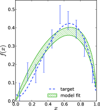
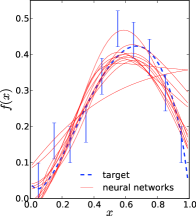
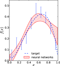
This function is plotted in Fig. 2 as a thick dashed line and labeled as “target”.

Next, $n_{\rm pts}$=10 fake data points $(x_{i},y_{i}\pm\Delta y_{i})$ are generated equidistantly in $x$. Their mean values $y_{i}$ are smeared around target values by random Gaussian fluctuations with standard deviation $\Delta y_{i}$=0.05, which is also taken to be the uncertainty of generated points. These fake data are then used for fits, first using the standard least-squares method with a two-parameter model

$$f(x)=x^{p_{1}}(1-x)^{p_{2}}\;,$$ (4)

and, second, utilizing the neural network method. Note that the Monte Carlo method of error propagation, which we use together with neural network fitting, itself requires to generate artificial data sets. Thus, we generated $N_{rep}$=12 replicas from original fake data and used them to train 12 neural networks that represent 12 functions, plotted as thin solid lines on the second panel of Fig. 2. These functions define a probability distribution in the space of functions $f(x)$ which, according to Eqs. (1–2), provides an estimate of the sought function $\tilde{f}(x)$, together with its uncertainty. This estimate is shown on the right panel of Fig. 2 as a (red) band with ascending hatches. The corresponding model fit result, obtained by the standard method of least-squares optimization and error propagation using the Hessian matrix, is shown in the left panel of Fig. 2 as a (green) band with descending hatches.

We have deliberately chosen the ansatz (4) with two properties, incorporating theoretical biases about endpoints: $f(1)=0$ and $f(0)=0$. The first of these actually “corresponds to the truth”, i.e., to Eq. (3), whereas the second one is erroneous. As a result, for $x\to 1$ the model fit is in much better agreement with the target function (thick dashed line) than neural networks, which rely only on data and are insensitive to this endpoint behaviour. On the other side, for $x\to 0$ the model fit is in some small disagreement with the target function, and, what is much worse, it very much underestimates the uncertainty of the fitted function there (the uncertainty becomes zero at endpoints!), demonstrating the dangers of unwarranted theoretical prejudices.

We can be more quantitative and say that according to the standard $\chi^{2}$ measure,

$${\chi}^{2}\equiv\sum_{i}^{n_{\rm pts}}\frac{(y_{i}-f(x_{i}))^{2}}{\Delta y_{i}^{2}}\;,$$

both methods lead to functions that correctly describe data:

$$\chi^{2}_{\rm model}/n_{\rm pts} =11.9/10\;;$$

$$\chi^{2}_{\rm neur.net}/n_{\rm pts} =12.3/10\;.$$

We can now further ask to what extent the two methods extract the underlying target function $\tilde{f}(x)$. Naturally, we can measure this by a kind of $\bar{\chi}^{2}$ criterion

$$\bar{\chi}^{2}\equiv\sum_{i}^{n_{\rm pts}}\frac{(\tilde{f}(x_{i})-f(x_{i}))^{2}}{\Delta f(x_{i})^{2}}\;,$$

where the denominator is now the propagated uncertainty $\Delta f(x_{i})$ rather than the experimental one $\Delta y_{i}$. In our toy example we get

$$\bar{\chi}^{2}_{\rm model}/n_{\rm pts} =25.6/10\;;$$

$$\bar{\chi}^{2}_{\rm neur.net}/n_{\rm pts} =8.4/10\;,$$

showing that the model fit underestimates its uncertainties, while neural networks are much more realistic.

Figure 3: Neural network extraction of $\operatorname{\mathfrak{Im}}{\cal H}(x_{\rm Bj},t)$ and $\operatorname{\mathfrak{Re}}{\cal H}(x_{\rm Bj},t)$ (ascending hatches, red) from HERMES data [21] compared with model fits (descending hatches, green) for two different values of momentum transfer squared $t$.

This example shows that the neural network method has a clear advantage if we want bias-free propagation of information from experimental measurements into the CFFs. Still, if we want to use some additional input, e.g., if we rely on the spectral property (3), we can do so also within the neural network method. For example, we could take the output of neural networks in this toy example not as an representation of the function $f(x)$ itself, but as representing $f(x)/(1-x)^{p}$, with some positive power $p$. Then the final neural network predictions for $f(x)$ would also be constrained by Eq. (3), without any further loss of generality (in practice it turns out that the dependence of the results on the choice of power $p$ is small). Various methods of implementing theoretical constraints in the neural network fitting method are discussed in Sect. 5.2.4 of [18].

4 Application to HERMES data

To extract the CFF $\mathcal{H}$ from asymmetries [21], measured by the HERMES collaboration in photon electroproduction off unpolarized protons, we applied the described neural network fitting method in [14]. We used 36 data points: 18 measurements of the first sine harmonic $A_{LU}^{\sin\phi}$ of the beam spin asymmetry, and 18 measurements of the first cosine harmonic $A_{C}^{\cos\phi}$ of the beam charge asymmetry. As for the toy model from the previous section, we compare the results with the standard least-squares model fit. Let us first shortly describe this model fit of $\mathcal{H}$. For the partonic decomposition of the imaginary part $\operatorname{\mathfrak{Im}}\mathcal{H}$ we used a model, presented in [10]:

$$\operatorname{\mathfrak{Im}}{\cal H}(x_{\rm Bj},t)=\pi\left[H^{\rm val}(\xi,\xi,t)+\frac{2}{9}H^{\rm sea}(\xi,\xi,t)\right].$$

Here, $H^{\rm a}(\xi,\xi,t)$ are GPDs along the cross-over trajectory $\xi=x$, parameterized as:

$$H(x,x,t)=\frac{n\,r}{1+x}\left(\frac{2x}{1+x}\right)^{-\alpha(t)}\\ \times\left(\frac{1-x}{1+x}\right)^{b}\frac{1}{\left(1-\frac{1-x}{1+x}\frac{t}{M^{2}}\right)^{p}}\;.$$

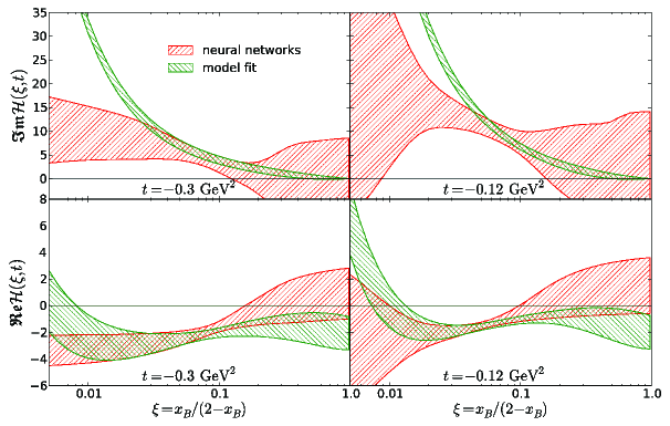
The parameters of $H^{\rm sea}$ were fixed by separate fits [10] to collider data, and some parameters of $H^{\rm val}$ were also fixed using information from DIS data and Regge trajectories $\alpha(t)$. The real part $\operatorname{\mathfrak{Re}}\mathcal{H}$ is expressed in terms of the imaginary one via a dispersion integral [22, 7, 23, 24] and the subtraction constant $C$, leaving us finally with a model that possesses four parameters: $r^{\rm val}$, $b^{\rm val}$, $M^{\rm val}$ and $C$. This model is fitted to experimental data, resulting in parameter values, which can be found in [14], and shapes of $\operatorname{\mathfrak{Im}}\mathcal{H}$ and $\operatorname{\mathfrak{Re}}\mathcal{H}$ that are plotted on Fig. 3 as (green) bands with descending hatches.

The neural network fit was performed by creating 50 neural networks with two neurons in the input layer (corresponding to kinematical variables $x_{B}$ and $t$), 13 neurons in the hidden middle layer, and two neurons in the output layer (corresponding to $\operatorname{\mathfrak{Im}}\mathcal{H}$ and $\operatorname{\mathfrak{Re}}\mathcal{H}$), cf. Fig. 1. These were trained on $N_{rep}$=50 Monte Carlo replicas of HERMES data. We checked that the resulting CFF $\cal H$ does not depend significantly on the precise number of neurons in the hidden layer. The results are also presented on Fig. 3, where we show the neural network representation of $\operatorname{\mathfrak{Im}}\mathcal{H}$ and $\operatorname{\mathfrak{Re}}\mathcal{H}$ as (red) bands with ascending hatches.

Comparing the two approaches, one notices that in the kinematic region of experimental data (roughly the middle-$x_{B}$ parts of Fig. 3 panels) neural network and model fit results coincide, i.e., error bands are of similar width and they overlap consistently. However, outside of this data region, we see that the predictions of the two approaches can be different. There the uncertainty of the model fit is in general smaller, and we observe a strong disagreement in the low $x_{B}$ region, reflecting the theoretical bias of the chosen model that possesses a $x^{-\alpha(t)}$ Regge behavior. The lesson learned from the toy model example is that, even if we believe in Regge behaviour for small $x_{B}$, we should still consider the uncertainty from the neural network method as more realistic.

5 Conclusion

Utilizing both a simplified toy example and HERMES measurements of photon electroproduction asymmetries, we demonstrated that neural networks and Monte Carlo error propagation provide a powerful and unbiased tool that extracts information from data. Comparisons with standard least-squares model fits reveal that the uncertainties, obtained from neural network fits, are reliable and realistic.

Relying on the hypothesis of $\mathcal{H}$ dominance, we found the CFF $\mathcal{H}$ from a completely unconstrained neural network fit. It is expected that the extraction of all four leading twist-two CFFs ($\mathcal{H}$, $\mathcal{E}$, $\widetilde{\mathcal{H}}$ and $\widetilde{\mathcal{E}}$, or the corresponding GPDs) from presently or soon-to-be available data will still be an ill-defined optimization problem. Thus, it might be necessary to implement in neural network fits some carefully chosen theoretically robust constraints, such as dispersion relations, sum rules [24] and lattice input.

References

- [1] D. Müller, D. Robaschik, B. Geyer, F. M. Dittes and J. Hořejši, Fortschr. Phys. 42, 101 (1994), [hep-ph/9812448].
- [2] A. V. Radyushkin, Phys. Lett. B380, 417 (1996), [hep-ph/9604317].
- [3] X.-D. Ji, Phys. Rev. D55, 7114 (1997), [hep-ph/9609381].
- [4] X.-D. Ji, Phys. Rev. Lett. 78, 610 (1997), [hep-ph/9603249].
- [5] M. Diehl and A. Schäfer, Phys. Lett. B698, 389 (2011), [1102.3081].
- [6] M. Diehl, D. Ostermeier and A. Schafer, 1111.0910.
- [7] K. Kumerički, D. Müller and K. Passek-Kumerički, Nucl. Phys. B794, 244 (2008), [hep-ph/0703179].
- [8] S. V. Goloskokov and P. Kroll, Eur. Phys. J. C53, 367 (2008), [0708.3569].
- [9] M. Guidal, Eur. Phys. J. A37, 319 (2008), [0807.2355].
- [10] K. Kumerički and D. Müller, Nucl. Phys. B841, 1 (2010), [0904.0458].
- [11] M. Guidal and H. Moutarde, Eur. Phys. J. A42, 71 (2009), [0905.1220].
- [12] M. Guidal, Phys. Lett. B689, 156 (2010), [1003.0307].
- [13] H. Moutarde, Phys. Rev. D79, 094021 (2009), [0904.1648].
- [14] K. Kumerički, D. Müller and A. Schäfer, JHEP 07, 073 (2011), [1106.2808].
- [15] S. Forte, L. Garrido, J. I. Latorre and A. Piccione, JHEP 05, 062 (2002), [hep-ph/0204232].
- [16] NNPDF, R. D. Ball et al., Nucl. Phys. B809, 1 (2009), [0808.1231].
- [17] NNPDF, R. D. Ball et al., Nucl.Phys. B838, 136 (2010), [1002.4407].
- [18] J. C. Rojo, hep-ph/0607122, PhD Thesis.
- [19] K. Kumerički, D. Müller and A. Schäfer, 1110.3798.
- [20] W. T. Giele, S. A. Keller and D. A. Kosower, hep-ph/0104052.
- [21] HERMES, A. Airapetian et al., JHEP 11, 083 (2009), [0909.3587].
- [22] O. V. Teryaev, hep-ph/0510031.
- [23] M. Diehl and D. Y. Ivanov, Eur. Phys. J. C52, 919 (2007), [0707.0351].
- [24] K. Kumerički, D. Müller and K. Passek-Kumerički, Eur. Phys. J. C58, 193 (2008), [0805.0152].