Majorana Fermions and Exotic Surface Andreev Bound States in Topological Superconductors: Application to Cu_xBi₂Se₃

Abstract

The recently discovered superconductor Cu_xBi₂Se₃ is a candidate for three-dimensional time-reversal-invariant topological superconductors, which are predicted to have robust surface Andreev bound states hosting massless Majorana fermions. In this work, we analytically and numerically find the linearly dispersing Majorana fermions at $k=0$, which smoothly evolve into a new branch of gapless surface Andreev bound states near the Fermi momentum. The latter is a new type of Andreev bound states resulting from both the nontrivial band structure and the odd-parity pairing symmetry. The tunneling spectra of these surface Andreev bound states agree well with a recent point-contact spectroscopy experimentando and yield additional predictions for low temperature tunneling and photoemission experiments.

The discovery of topological insulators has generated much interest in not only understanding their properties and potential applications to spintronics and thermoelectrics but also searching for new topological phases. A particularly exciting avenue is topological superconductorsludwig ; kitaev ; read ; roy ; zhangtsc ; volovik ; yip ; moore ; nagaosa , in which unconventional pairing symmetries lead to topologically ordered superconducting ground statesfuberg ; sato ; qihugheszhang . The hallmark of a topological superconductor is the existence of gapless surface Andreev bound states which host itinerant Bogoliubov quasiparticles. These quasiparticles are solid-state realizations of massless Majorana fermions.

There is currently an intensive search for topological superconductors. In particular, a recently discovered superconductor Cu_xBi₂Se₃ with $T_{c}\sim 3K$cava has attracted much attentionpalee . A theoretical studyfuberg proposed that the strong spin-orbit coupled band structure of Cu_xBi₂Se₃ favors an odd-parity pairing symmetry, which leads to a time-reversal-invariant topological superconductor in three dimensions. Subsequently, many experimental and theoretical effortswray ; heat ; sample ; magnetization ; haolee have been made towards understanding superconductivity in Cu_xBi₂Se₃. In a very recent point-contact spectroscopy experiment, Sasaki et al.ando have observed a zero-bias conductance peak which strongly indicates unconventional pairingabs .

In this Letter, we find a new branch of gapless surface Andreev bound states (SABS), in addition to linearly dispersing Majorana fermions at ${\bf k}=0$, in the topological superconducting phase of Cu_xBi₂Se₃ and related doped semiconductors. This new branch of SABS is located near the Fermi momentum and is protected by a new bulk topological invariant. Moreover, they result in unique features in the tunneling spectra which are in good agreement with the point-contact spectroscopy experiment on Cu_xBi₂Se₃ando . We conclude by predicting clear signatures of these SABS, which can be tested in future tunneling and photoemission experiments at low temperatures.

We start from the $k\cdot p$ Hamiltonian for the band structure of Cu_xBi₂Se₃ near $\Gamma$fuberg

$$H({\bf k})=m\sigma_{x}+v_{z}k_{z}\sigma_{y}+v\sigma_{z}(k_{x}s_{y}-k_{y}s_{x}).$$ (1)

Here $\sigma_{z}=\pm 1$ labels the two Wannier functions which are primarily $p_{z}$ orbitals (from Se and Bi atoms) on the upper and lower part of the quintuple layer (QL) unit cell respectively (see Fig.1). Each orbital has a two-fold spin degeneracy labeled by $s_{z}=\pm 1$. We note that an earlier $k\cdot p$ Hamiltonianzhang violates the mirror symmetry of the lattice, and a corrected versionliu is consistent with (1). Detailed discussion of the discrepancy is left to Supplementary Materialdetail . The sign of $mv_{z}$ is a crucial quantity which will now be inferred from the existence of surface states near $k_{x}=k_{y}=0$ in the surface Brillouin zone.

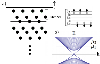
Figure 1: a) Side view of a semi-infinite crystal of Bi₂Se₃. The two relevant $p_{z}$ orbitals are shown in the zoom-in view of the QL unit cell. b) Bulk and surface bands of the tight-binding model for Bi₂Se₃. $\mu_{1}$ and $\mu_{2}$ denote two chemical potentials where the surface states have, respectively, not merged and merged into the bulk bands.

Consider a semi-infinite Cu_xBi₂Se₃ crystal occupying $z<0$, which is naturally cleaved between QLs (see Fig.1). The realistic boundary condition corresponding to such a termination in the continuum $k\cdot p$ theory isfuberg

$$\sigma_{z}\psi(z=0)=\psi(z=0).$$ (2)

This boundary condition reflects the vanishing of the electron wavefunction on the bottom layer ($\sigma_{z}=-1$) at $z=0$. Solving the differential equation

$$E\psi = H(k_{x},k_{y},-i\partial_{z})\psi$$ (3)

subject to (41), we find two branches of mid-gap states

$$\psi_{\pm}(k_{x},k_{y},z) = e^{z/l}(1,0)_{\sigma}\otimes(1,\pm ie^{i\phi})_{s},$$ (4)

where $l=-v_{z}/m$ is the decay length, $\phi$ is the azimuthal angle of $(k_{x},k_{y})$, and the subscripts $\sigma$ and $s$ denote the orbital $\sigma_{z}$ and spin $s_{z}$ basis. For $v_{z}m>0$, there are no decaying solutions; only when $v_{z}m<0$ in (4) do we obtain surface states decaying in the $-z$ direction. The dispersion of these surface states is $E_{\pm}(k_{x},k_{y})=\pm v\sqrt{k_{x}^{2}+k_{y}^{2}}\equiv\pm vk$, which agree well with the photoemission data from Cu_xBi₂Se₃wray . Thus, the existence of surface states on surfaces terminated between QLs establishes $v_{z}m<0$ in $H({\bf k})$ for Cu_xBi₂Se₃detail .

Having established that $v_{z}m<0$ and $v$ parameterizes the linear dispersion of the surface states, we now turn to the superconducting state of Cu_xBi₂Se₃. Ref.fuberg classified four different pairing symmetries compatible with short-range pairing interactions, and found that a spin-triplet, orbital-singlet, odd-parity pairing symmetry is favored when the inter-orbital attraction exceeds the intra-orbital one. The mean-field Hamiltonian of this superconducting state is

$$H_{\rm MF} = \int d{\bf k}[c_{{\bf k}}^{\dagger},\bar{c}_{-{\bf k}}]{\cal H}({\bf k})\left[\begin{array}[]{c}c_{{\bf k}}\\ \bar{c}_{-{\bf k}}^{\dagger}\end{array}\right],$$ (7)

$${\cal H}({\bf k}) = (H({\bf k})-\mu)\tau_{z}+\Delta\sigma_{y}s_{z}\tau_{x}.$$ (8)

Here $c_{{\bf k}}^{\dagger}=(c_{{\bf k},1\uparrow}^{\dagger},c_{{\bf k},1\downarrow}^{\dagger},c_{{\bf k},2\uparrow}^{\dagger},c_{{\bf k},2\downarrow}^{\dagger})$ and $\bar{c}_{-{\bf k}}\equiv c_{-{\bf k}}\cdot is_{y}$ are four-component electron operators, with the subscript $1,2$ labeling the two orbitals (Fig.1a). In the Bogoliubov-de Gennes Hamiltonian ${\cal H}({\bf k})$, $\tau_{x}$ and $\tau_{z}$ are Pauli matrices in Nambu space, $\Delta$ is the pairing potential, and $\mu>|m|$ is the chemical potential in the conduction band.

The above odd-parity superconducting Cu_xBi₂Se₃ is fully-gapped in the bulk but has topologically protected surface Andreev bound states. To determine the wavefunction and dispersion of these bound states, we begin by solving the BdG Hamiltonian ${\cal H}(k_{x},k_{y},-i\partial_{z})$ for the SABS at $k_{x}=k_{y}=0$. We find a Kramers pair of $\epsilon=0$ eigenstatesdetail :

$$\psi_{k=0,\alpha}(z) = e^{z\cdot\Delta/|v_{z}|}(\sin(k_{F}z-\theta),\sin(k_{F}z))_{\sigma}$$ (9)

$$\otimes \left[(1,-\alpha)_{s},i{\rm sgn}(v_{z})(1,\alpha)_{s}\right]_{\tau},\;\alpha=\pm 1$$

Here $k_{F}\equiv\sqrt{\mu^{2}-m^{2}}/v_{z}$ is Fermi momentum in the $z$ direction, and $\theta$ is defined by $e^{i\theta}=(m+i\sqrt{\mu^{2}-m^{2}})/\mu$. The subscript $\tau$ denotes a Nambu spinor. The Bogoliubov quasiparticle at $k=0$ is defined by $\gamma_{\alpha}=\int dz\;\psi_{k=0,\alpha}(z)(c^{\dagger}(z),\bar{c}(z))_{k=0}^{T}.$ It is straight-forward to verify that $\gamma_{\alpha}^{\dagger}=\gamma_{\alpha}$ up to an unimportant overall phase. This means that such quasiparticles are two-component massless Majorana fermions in $2+1$ dimensions.

Having found the SABS wavefunction at $\epsilon=0$, $k=0$, we now show that the SABS dispersion crosses $\epsilon=0$ again at ${\it finite}$ $k$, which is one of the main results of this paper. We establish this second crossing in two different ways: first, by a direct calculation, and second, by a topological argument. It will become evident that the two approaches yield complementary information.

In the direct approach, we search for a second crossing by asking for which $k_{0}>0$ does ${\cal H}(0,k_{0},-i\partial_{z})\psi=0$ have a solution (it suffices to consider $k_{x}=0,k_{y}\equiv k_{0}>0$ only, due to rotational invariance). We find that $k_{0}$ is the nontrivial solution of the algebraic equationdetail

$$|x|^{2}+2{\rm sgn}(v_{z})\frac{E_{F}}{m}{\rm Re}(x)-1=0,$$ (10)

where $x$ is defined as

$$x\equiv\frac{vk_{0}-i(\Delta+iE_{F})}{\sqrt{(vk_{0})^{2}+(\Delta+iE_{F})^{2}}},\;E_{F}\equiv\sqrt{\mu^{2}-m^{2}}.$$ (11)

For Cu_xBi₂Se₃ in the normal state with $\Delta=0$ and $v_{z}m<0$, the above equation has a solution $k_{0}=\mu/v$, which exactly correspond to the topological insulator surface states at Fermi energy obtained earlier in (4). With superconductivity, topological surface states in the normal state turn into SABS, with their location $k_{0}$ and wavefunction $\psi_{k_{0},\alpha}$ perturbed by $\Delta$: $k_{0}\simeq\frac{\mu}{v}(1-\frac{\Delta^{2}}{2m^{2}})$ and $\psi_{k_{0},\alpha}$ acquires particle-hole mixing to first order in $\Delta$. Due to rotational invariance of the $k\cdot p$ Hamiltonian, the second crossing, hereafter denoted by $k_{0}$, exists along all directions in the $xy$ plane. This leads to a Fermi surface of SABS.

In the topological approach, we first solve for the SABS dispersion at small $k$ and use topological arguments to infer its behavior at large $k$. Again, we set $k_{x}=0$ for convenience. Treating the $k_{y}$-dependent term in $H_{\rm BdG}$ as a perturbation, we find the dispersion is linear near $k=0$: $\epsilon_{\alpha}(k)=\alpha\tilde{v}k+o(k^{3})$, forming a Majorana cone. The velocity $\tilde{v}$ is given by:

$$\tilde{v} = v\frac{\Delta^{2}+{\rm sgn}(v_{z})\Delta m}{\Delta^{2}+{\rm sgn}(v_{z})\Delta m+\mu^{2}}\simeq v\cdot{\rm sgn}(v_{z})\frac{m\Delta}{\mu^{2}}.$$ (12)

In the second equality, we have used the fact $\Delta\ll|m|<\mu$ for weak-coupling superconductors.

In (12), it is important that the SABS velocity $\tilde{v}$ at $k=0$ has an opposite sign from the band velocity $v$ in the normal state of the doped topological insulator Cu_xBi₂Se₃ ($v_{z}m<0$). As we now show, this fact has crucial implications for the SABS dispersion away from $k=0$: the two branches of SABS $\psi_{k,\pm}$ must cross each other at $\epsilon=0$ an odd number of times between $\bar{\Gamma}$ and the surface Brillouin zone edge $\bar{M}$. The existence of such additional crossings is dictated by a topological invariant we call “mirror helicity”, which is a generalization of mirror Chern numberteofukane in topological insulators to topological superconductors. To define this invariant, note that the crystal structure of Cu_xBi₂Se₃ has a mirror reflection symmetry $x\rightarrow-x$. As a result, the band structure (1) is invariant under mirror. However, the pairing potential in (8) changes sign under mirror reflection. So the BdG Hamiltonian is invariant under a mirror reflection combined with a $Z_{2}$ gauge transformation $\Delta\rightarrow-\Delta$:

$${\cal H}(k_{x},k_{y},k_{z}) = \tilde{M}{\cal H}(-k_{x},k_{y},k_{z})\tilde{M}^{-1},$$ (13)

Here $\tilde{M}=M\tau_{z}$, $M=-is_{x}$ represents mirror reflection on electron spin. Because of this generalized mirror symmetry, bulk states are grouped into two classes with mirror eigenvalues $\pm i$ respectively. Each class can have a nonzero Chern number $n_{\pm i}$. Time reversal symmetry requires $n_{+i}=-n_{-i}$. The magnitude $|n_{+i}|=|n_{-i}|$ determines the number of helical Andreev modes with $k_{x}=0$ on the edge of $yz$ plane, while the sign defines a $Z_{2}$ mirror helicity: $\eta\equiv{\rm sgn}(n_{+i})=-{\rm sgn}(n_{-i}).$ The bulk topological invariant $\eta$ determines the helicity of such Andreev modes. For instance, $\eta<0$ implies that the mode with mirror eigenvalue $-i$($+i$) moves clockwise(anti-clockwise) with respect to $+x$ axis at the edge of the $yz$ plane, and its energy-momentum dispersion curve must eventually merge into the $E>0$ bulk quasiparticle continuum at a large positive(negative) momentum. Similar bulk-boundary correspondence applies to surface states in topological insulatorsteofukane ; murakami .

As we show in Supplementary Materialdetail , the topological superconducting phase of Cu_xBi₂Se₃ and the undoped topological insulator Bi₂Se₃ have the same mirror helicity $\eta$, which is determined by the sign of the Dirac band velocity $v$ in the bulk. Given the relation between $\eta$ and helicity of surface excitations, this implies that the SABS in Cu_xBi₂Se₃ must have the same helicity as surface states in Bi₂Se₃. On the other hand, the SABS velocity $\tilde{v}$ at $k=0$ has an opposite sign from the Dirac band $v$. To reconcile this fact with the helicity requirement, the two SABS branches $\psi_{k,\alpha}$—which are mirror eigenstates with eigenvalues $\tilde{M}=i\alpha$—must become twisted and switch places before merging into the bulk. This necessarily results in an odd number of crossings between $\bar{\Gamma}$ and $\bar{M}$.

The above topological argument reveals the robustness of gapless SABS at the second crossing in the $k\cdot p$ regime and beyond. In the $k\cdot p$ regime, the surface states at ${\bf k}$ and $-{\bf k}$ have opposite mirror eigenvalues (or spins) due to their helical nature, whereas the pairing symmetry $\Delta$ only pairs states with the same mirror eigenvalues. This symmetry incompatibility makes the surface states remain gapless in the topological superconducting phase mirror . Moreover, the topological argument demonstrates that the second crossing is topologically protected by the mirror helicity invariant in the bulk, as long as $\tilde{v}/v<0$ at $k=0$. As a result, the second crossing remains in a much larger energy range, even when higher order corrections to the $k\cdot p$ Hamiltonian become important, as shown below. In particular, we emphasize that the existence of the second crossing is independent of whether surface states are separated from the bulk at the Fermi energy.

To gain more insight into these twisted SABS and to calculate their local density of states, we explicitly obtain its dispersion in the entire surface Brillouin zone. For this purpose, we construct a two-orbital tight-binding model in the rhombohedral lattice shown in Fig.1 and calculate the SABS dispersion numerically. Details of our tight-binding model and its distinction from previous modelsando ; haolee are described in the Supplementary Materialdetail .

Here we would like to note the following aspects of our model. The normal state tight-binding model is constructed to reproduce both the $k\cdot p$ Hamiltonian (1) of Cu_xBi₂Se₃ in the small $k$ limit and the boundary condition (41) in the continuum theory. The bulk and surface bands of the normal state tight-binding model are displayed in Figure 1b; at chemical potential $\mu_{1}$, the Fermi momentum is relatively small and terms higher order than ${\bf k}$ are negligible, whereas at $\mu_{2}$, these higher order terms cause deviation from the $k\cdot p$ Hamiltonian.

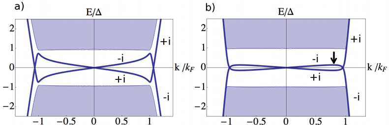
Figure 2: SABS dispersion for the tight-binding model in which a) $m=-0.3<0$, $\mu_{1}=0.6$ and b) $m=-0.3<0$, $\mu_{2}=1$; The mirror eigenvalues are displayed near each branch of SABS. The SABS twist with a second crossing near Fermi momentum, as also observed in Ref.haolee . The arrow denotes where the dispersion has zero slope, resulting in a Van Hove singularity in the density of states.

Upon adding odd-parity superconductivity pairing to the model, we obtain the SABS dispersion (Fig. 2). A branch of linearly dispersing Majorana fermions is found at $k=0$, which signifies a three-dimensional topological superconductor. In addition, the bands of Andreev bound states in the surface Brillouin zone are twisted: they connect the Majorana fermion at $k=0$ with the second crossing near Fermi momentum. Such behavior was independently found by Hao and Leehaolee ; detail , and its topological origin is revealed by our analytical calculations and arguments.

For a given branch ($\tilde{M}=\pm i$) of SABS, its particle-hole character evolves as a function of momentum from having an equal amount of particle and hole (charge neutral) at $k=0$ to being exclusively hole or particle (charged) at large $k$. At chemical potential $\mu_{1}$, the SABS near the second crossing can be identified with nearly unpaired surface states in the normal state, which show up twice—as particle and hole—in the BdG spectrum. However, even when these surface states have merged into the bulk, the SABS still has the second crossing, as required by the mirror helicity. This is shown in Fig. 2b, at chemical potential $\mu_{2}$. The resulting gapless SABS near the second crossing has substantially more particle-hole mixing than the first case and is unrelated to surface states in the normal state. Such SABS defy a quasi-classical description and represent a new type of Andreev bound states which arises from the interplay between nontrivial band structure and unconventional superconductivity.

Finally, we relate our findings of SABS in Cu_xBi₂Se₃ to the recent point-contact spectroscopy experimentando , in which a zero-bias differential conductance peak along with a dip near the superconducting gap edge was observed below $1.2$K and attributed to SABS. To compare with this experiment, we calculate the local tunneling density of states (LDOS) as a function of energy for $m/\mu_{2}=0.3$—roughly the value found in ARPESwray . The resulting LDOS at zero and finite temperatures are shown in Fig. 3. The finite temperature LDOS from $T=0.05\Delta$ to $T=0.2\Delta$ agrees with the experimentally observed differential conductance peaks as well as the dips with the slight asymmetry between positive and negative voltages. Both features along with the absence of coherence peaks contrast sharply with the tunneling spectrum of an s-wave superconductor.

In addition to comparison with the experiment, we make the following predictions stemming from the zero temperature LDOS in Figure 3a. Here the two peaks arise from Van Hove singularities at the particular energy near $E=0$ where the SABS bands have zero slope, indicated by the arrow in Fig. 2b. Furthermore, the significant asymmetry in the height of these two peaks reflects the fact that the SABS at the turning point is primarily of hole type, as noted earlier. The energy of these two peaks and the magnitude of their asymmetry depends somewhat on details of band structure. However, the existence of two peaks only depends on there being a turning point in the SABS dispersion, which is guaranteed by the existence of a second crossing in a wide regime of chemical potentials. Hence, we predict that for relatively clean surfaces the zero-bias conductance peak in the tunneling spectra will split into two asymmetric peaks at even lower temperatures. Such peaks will be an unambiguous signature of Majorana fermions smoothly turning into normal surface electrons. Furthermore, the SABS dispersion we predict in Fig.2 can be directly tested in future ARPES experiments.

Figure 3: Tunneling local density of states (arbitrary units) at a) $T=0$ and b) finite temperature. In both cases, the chemical potential is $\mu_{2}=1$.

While the main focus of this Letter is Cu_xBi₂Se₃, we end by discussing the implications of our findings for superconducting doped semiconductors with similar band structures. Candidates include Bi₂Te₃bite under pressure, TlBiTe₂thallium , PbTepbte , SnTesnte , and GeTegete . Provided that the material is inversion symmetric and its Fermi surface is centered at time-reversal-invariant momenta, the Dirac-type relativistic $k\cdot p$ Hamiltonian (1) describes their band structuresfukane . Moreover, if the pairing symmetry is odd under spatial inversion and fully gapped, the system is (almost) guaranteed to be a topological superconductor according to our criterionfuberg ; qifu . Our work is also relevant to noncentrosymmetric superconductors such as YPtBiyptbi , if their pairing symmetries have dominant odd-parity components.

As a final point which captures the essence of this work, we compare and contrast SABS in doped superconducting topological insulators with normal insulators, which differ by a band inversion ($v_{z}m<0$ versus $v_{z}m>0$). In both, the Majorana fermion SABS exist at $k=0$ as shown in (9, 12). However, the SABS in doped normal insulators do not necessarily have the second crossing near Fermi momentumdetail . This can be understood from our mirror helicity argument, with the difference being that $\tilde{v}/v>0$ for $v_{z}m>0$ (see Eq.(12)). In this sense, the new type of surface Andreev bound state and its phenomenological consequences are the unique offspring of both nontrivial band structure and odd-parity topological superconductivity.

Note: Two recent studieshaolee ; ando calculated the surface spectral function numerically in Cu_xBi₂Se₃ tight-binding models. The second crossing of SABS was independently found in Ref.haolee . We also learned of another point-contact measurement on Cu_xBi₂Se₃point .

Acknowledgement: We thank Yoichi Ando, Erez Berg, Chia-Ling Chien, Patrick Lee and Yang Qi for helpful discussions, as well as Anton Akhmerov and David Vanderbilt for helpful comments on the manuscript. This work is supported by DOE under cooperative research agreement Contract Number DE-FG02-05ER41360 and NSF Graduate Research Fellowship under Grant No. 0645960 (TH), the Harvard Society of Fellows and MIT start-up funds (LF). LF would like to thank Institute of Physics in China, and Institute of Advanced Study at Tsinghua University for generous hosting.

I Supplementary Material

I.1 I. SABS Wavefunction and Second Crossing

First, we derive in detail the wavefunction (6) in the main text from the BdG Hamiltonian ${\cal H}({\bf k})$. A Kramers pair of zero-energy eigenstates $\psi_{k=0,\alpha=\pm}(z)$ with mirror eigenvalues $\tilde{M}=i\cdot\alpha$ is expected from the topology and symmetry of ${\cal H}({\bf k}_{\parallel}=0)$. For a given mirror eigenstate, $s_{x}$ is locked to $\tau_{z}$ by the identity $s_{x}\tau_{z}=-\alpha$, so that $\psi_{k=0,\alpha}(z)$ satisfies a reduced $4$-component equation:

$$[(m\sigma_{x}-iv_{z}\sigma_{y}\partial_{z}-\mu)\tau_{z}+\Delta\sigma_{y}\tau_{x}]\psi_{k=0,\alpha}(z)=0.$$ (14)

This can be further simplified by multiplying both sides by $\tau_{z}$:

$$[m\sigma_{x}-iv_{z}\sigma_{y}\partial_{z}-\mu+i\Delta\sigma_{y}\tau_{y}]\psi_{k=0,\alpha}(z)=0.$$

It is evident that $\psi_{k=0,\alpha}$ is an eigenstate of $\tau_{y}$. The corresponding eigenvalue is given by ${\rm sgn}(v_{z})$ in order to have a decaying solution. Eq.(14) then reduces to a two-component equation in orbital space, which has two independent solutions:

$$\xi_{\pm}(z)=(1,e^{\pm i\theta})_{\sigma}\cdot e^{(\pm ik_{F}+\Delta/|v_{z}|)z}.$$ (15)

$\theta$ is defined by $e^{i\theta}=(m+i\sqrt{\mu^{2}-m^{2}})/\mu$. Choosing a suitable linear combination of $\xi_{+}$ and $\xi_{-}$ to satisfy the boundary condition (2) in the main text, we obtain the wavefunction of SABS, which is reproduced here for the reader’s convenience:

$$\psi_{k=0,\alpha}(z) = e^{z\cdot\Delta/|v_{z}|}(\sin(k_{F}z-\theta),\sin(k_{F}z))_{\sigma}$$

$$\otimes \left[(1,-\alpha)_{s},i{\rm sgn}(v_{z})(1,\alpha)_{s}\right]_{\tau},\;\alpha=\pm 1.$$

Next we solve for the location of the SABS second crossing. For convenience, we look for a zero-energy solution $\psi(z)$ at $k_{x}=0$, $k_{y}\equiv k_{0}$ with mirror eigenvalue $+i$ (i.e., $s_{x}\tau_{z}=-1$). $\psi$ satisfies

$$\left[(m\sigma_{x}-iv_{z}\sigma_{y}\partial_{z}-\mu)\tau_{z}+vk_{0}\sigma_{z}+\Delta\sigma_{y}\tau_{x}\right]\psi(z)=0$$ (16)

Recall that $v_{z}m<0$ for a doped topological insulator. Without loss of generality, here we choose $m<0,v_{z}>0$. By multiplying Eq.(16) by $i\sigma_{y}\tau_{z}$, the zero-energy solution satisfies

$$\left[m\sigma_{z}+v_{z}\partial_{z}-i\mu\sigma_{y}-vk_{0}\sigma_{x}\tau_{z}-\Delta\tau_{y}\right]\psi(z)=0.$$ (17)

We write the wavefunction $\psi(z)$ as

$$\psi(z)=e^{i\lambda\sigma_{x}/2}\phi(z),\;\lambda\in\rm C$$ (18)

where $\cos\lambda=\mu/E_{F}$ and $\sin\lambda=-im/E_{F}$, $E_{F}\equiv\sqrt{\mu^{2}-m^{2}}$. Eq.(16) then becomes

$$\left[v_{z}\partial_{z}-iE_{F}\sigma_{y}-vk_{0}\sigma_{x}\tau_{z}-\Delta\tau_{y}\right]\phi(z)=0$$ (19)

Note that Eq.(19) now commutes with $\sigma_{y}\tau_{y}$, which becomes a constant labeled by $\tau$. The reduced equation for $\phi_{\tau}(z)$ is

$$\left[v_{z}\partial_{z}-(\tau\Delta+iE_{F})\sigma_{y}-vk_{0}\sigma_{x}\right]\phi(z)=0.$$ (20)

The solution takes the form $\phi(z)=e^{Kz}\xi$. First consider $\tau=1$. From Eq. (20), we have

$$K_{\pm}=\frac{\pm\sqrt{(vk_{0})^{2}+(\Delta+iE_{F})^{2}}}{v_{z}}\equiv\pm E_{z}/v_{z}.$$ (21)

Corresponding eigenvectors are given by

$$\xi_{\pm}=(x_{\pm},1),\;x_{\pm}\equiv(vk_{0}-i(\Delta+iE_{F}))/(v_{z}K_{\pm})$$ (22)

To get a decaying solution, we must have ${\rm Re}(K)>0$. Hence, we must choose $K_{+}$ and thus $\xi_{+}$. We now rewrite the complete wavefunction with both orbital and Nambu components (spin is locked by $s_{x}\tau_{z}=-1$ and not shown explicitly):

$$\xi_{+} = \frac{x_{+}-i}{2}(1,i,i,-1)+\frac{x_{+}+i}{2}(1,-i,-i,-1)$$ (23)

$$= (x_{+},1,1,-x_{+})$$

Note that the equation for $\tau=-1$ is equivalent to the complex conjugate of that for $\tau=1$. Therefore if we choose $K_{+}\equiv K$ and $x_{+}\equiv x$ for $\tau=1$, we must choose $K^{*}$ and $x^{*}$ for $\tau=-1$. The corresponding wavefunction is

$$\xi^{*}=(x^{*},1,1,-x^{*})$$ (24)

It follows from Eqn. (18) that

$$\psi(\tau=1) = e^{i\lambda\sigma_{x}/2}(x,1,1,-x)$$

$$\psi(\tau=-1) = e^{i\lambda\sigma_{x}/2}(x^{*},1,-1,x^{*})$$ (25)

Up to normalization, the most general form of $\psi(z)$ satisfying the boundary condition (41) is

$$\psi(0)=(1,0,A,0),$$ (26)

where $A$ is some constant. Hence, for a nontrivial solution to exist, the determinant of the $2\times 2$ matrix made from the second and fourth component of $\psi(\tau=1)$ and $\psi(\tau=-1)$ must be zero. This condition is simplified to an algebraic equation

$$0 = 2{\rm Re}(x)+\frac{m}{E_{F}}(-1+|x|^{2})$$ (27)

which is the result cited in the main text. Our previous solution at $k=0$ (9) corresponds to $x=\pm i$, which satisfies the above condition. Another simple limit is the normal state with $\Delta=0$. In this case, the second crossing is simply located at the momentum where the topological insuator surface states cross the chemical potential, namely, $k_{0}=\mu/v$. We can check that for this case, $x=(\mu+E_{F})/(-m)$ indeed satisfies Eq. (27). Now we solve for $k_{0}$ to first order in $\Delta$. Temporarily absorbing $v$ into $k_{0}$ and expanding $x$ to second order in $\Delta$, we obtain

$${\rm Re}(x) = \frac{E_{F}+k_{0}}{\sqrt{-E_{F}^{2}+k_{0}^{2}}}$$

$$+\frac{(-2E_{F}k_{0}-k_{0}^{2})\Delta^{2}}{2(E_{F}-k_{0})^{2}(E_{F}+k_{0})\sqrt{-E_{F}^{2}+k_{0}^{2}}}$$

$${\rm Im}(x) = \frac{k_{0}\Delta}{(E_{F}-k_{0})\sqrt{\-E_{F}^{2}+k_{0}^{2}}}$$

$$\frac{m}{E_{F}}(|x|^{2}-1) = \frac{-2m}{E_{F}-k_{0}}+\frac{2mk_{0}\Delta^{2}}{(E_{F}-k_{0})^{3}(E_{F}+k_{0})}$$

From Eq.(27), we then extract the leading order to correction to $k_{0}$:

$$k_{0}=\frac{\mu}{v}(1-\frac{\Delta^{2}}{2m^{2}}).$$ (28)

The corresponding $x$ at $k_{0}$ is given

$${\rm Re}(x) = \frac{m}{-\mu+E_{F}}-\frac{\Delta^{2}\mu(\mu+E_{F})}{2m^{3}(-\mu+E_{F})}$$ (29)

$${\rm Im}(x) = -\frac{\Delta\mu}{m(-\mu+E_{F})}$$ (30)

We conclude this section by calculating the ratio of the particle ($\tau=1$) and hole ($\tau=-1$) components of the $s_{x}\tau_{z}=-1$ wavefunction $\psi(z)$ at the second crossing and at $z=0$. This wavefunction is some linear combination $c_{1}\psi(\tau=1)+c_{2}(\tau=-1)$ with vanishing second and fourth components (to satisfy the boundary condition). Hence, we find

$$\frac{c_{2}}{c_{1}}=\frac{-(\cos(\lambda/2)+ix\sin{\lambda/2})}{\cos{\lambda/2}+ix^{*}\sin{\lambda/2}}$$ (31)

The hole/particle ratio is

$$r\equiv\frac{\cos{\lambda/2}(c_{1}-c_{2})-i\sin{\lambda/2}(c_{1}x-c_{2}x^{*})}{\cos(\lambda/2)(c_{1}x+c_{2}x^{*})+i\sin(\lambda/2)(c_{1}+c_{2})}$$ (32)

Using the fact that the second and fourth components vanish, which is equivalent to

$$\cos{\lambda/2}(c_{1}+c_{2})+i\sin{\lambda/2}(c_{1}x+c_{2}x^{*})=0$$ (33)

$$-\cos{\lambda/2}(c_{1}x-c_{2}x^{*})+i\sin{\lambda/2}(c_{1}-c_{2})=0,$$ (34)

we get

$$r=\frac{c_{1}-c_{2}}{(c_{1}+c_{2})(i\cot(\lambda/2))}=\frac{1+i(\tan{\lambda/2}){\rm Re}(x)}{i{\rm Im}(x)}$$ (35)

Recalling that $\cos\lambda=\mu/E_{F}$ and $\sin\lambda=-im/E_{F}$, we have

$$\tan(\lambda/2)=\frac{e^{i\lambda}-1}{i(e^{i\lambda}+1)}=\frac{\mu+m-E_{F}}{\mu+m+E_{F}}$$ (36)

The hole/particle ratio at the second crossing is thus

$$r=\frac{\Delta(\mu+E_{F})(\mu+m-E_{F})}{2im^{2}(\mu+m+E_{F})},$$ (37)

which is first order in $\Delta$.

I.2 II. Mirror Helicity

Here we show that the topological insulator and topological superconductor phases have the same mirror helicity. We deduce this fact from the phase transition between topological insulators and topological superconductors.

The BdG Hamiltonian (5) in the main text exhibits three topologically distinct gapped phases as a function of the band gap, pairing potential and doping. At zero doping ($\mu=0$) and in the absence of superconductivity ($\Delta=0$), the system is either an normal band insulator or a topological insulator, depending on the sign of $m$. At finite electron doping, the chemical potential lies inside the conduction band: $\mu>0$. When the odd-parity pairing $\Delta$ occurs in such a doped normal insulator or topological insulator, the system becomes a fully gapped topological superconductor. For the sake of our argument,we note that the topological superconductor phase is adiabatically connected to the $\mu=0$ and $\Delta>|m|$ limit. Fig.4 shows the three phases in the $\mu=0$ phase diagram as a function of $m$ and $\Delta$. The phase transition between topological superconductors and normal/topological insulators occurs at $\Delta=\pm m$.

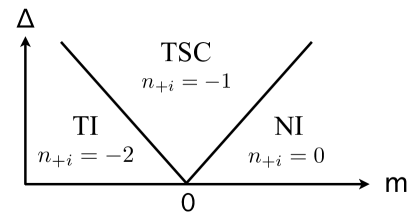
Figure 4: Phase diagram of fully-gapped odd-parity superconductivity in doped semiconductors as a function of band gap $m$ and pairing potential $\Delta$, showing three gapped phases: band insulator, topological insulator and topological superconductor. They are topologically distinguished by the mirror Chern numbers $n_{+i}$.

Recall from the main text that due to mirror symmetry, each phase has a mirror Chern number $n_{+i}=n_{-i}$ displayed in Fig. 4. Using $n_{+i}=0$ for the normal insulator as a reference, we can obtain the mirror Chern number for the topological insulator and topological superconductor by calculating the change of $n_{+i}$ across the phase transition to the normal insulator. Due to the double counting of particles and holes, the mirror Chern number of a band insulator defined in Nambu space is always an even integer twice the value of that defined previously for insulators in Ref.[25]. As a result, a direct transition from topological insulator to band insulator at $\Delta=0$ changes $n_{+i}$ by two. For $\Delta\neq 0$, this transition is split into two transitions with an intermediate topological superconductor phase, so that each transition changes $n_{+i}$ by one. Therefore we have

$$n_{+i}({\rm TI})=2n_{+i}({\rm TSC}).$$ (38)

Recall that mirror helicity is defined as $\eta\equiv{\rm sgn}(n_{+i})$. Hence, the topological insulator and topological superconductor phase have the same mirror helicity.

I.3 III. Tight-binding Model

Here we present the details of our tight-binding model. This model is defined on the rhombohedral lattice with a bilayer unit cell shown in Fig.1. The Hamiltonian $H=H_{0}+H_{12}+H_{\rm soc}+H^{\prime}_{12}$ consists of the following four terms.

$$H_{0}=\sum_{<ij>}t_{0}c_{i\alpha}^{\dagger}c_{j\alpha}$$

describes nearest neighbor hopping within the same layer.

$$H_{12}=\sum_{<i\in 1,j\in 2>}t_{1}c_{i\alpha}^{\dagger}c_{j\alpha}+\sum_{<i\in 1,j^{\prime}\in 2>}t_{2}c_{i\alpha}^{\dagger}c_{j^{\prime}\alpha}$$ (39)

describes hopping between two adjacent layers within a QL ($t_{1}$) and on two neighboring QLs ($t_{2}$). $t_{0}$, $t_{1}$ and $t_{2}$ are spin-independent. In addition, the two orbitals in the upper and lower part of the unit cell (Fig.1a) experience local electric fields along the $\pm z$ direction, which give rise to the following Rashba-type spin-orbital associated with intra-layer hopping:

$$H_{\rm soc} = (\sum_{<ij>\in 1}-\sum_{<ij>\in 2})\frac{i\lambda}{2}c_{i\alpha}^{\dagger}{\vec{s}}_{\alpha\beta}c_{j\beta}\cdot(\hat{z}\times\mathbf{a}_{ij}),$$

where $\mathbf{a}_{ij}=\frac{1}{2}\epsilon_{ijk}(\mathbf{R}_{j}-\mathbf{R}_{k})$ denote the vectors joining nearest neighbors within a layer, and $\mathbf{R}_{1,2,3}$ are the Bravais lattice vectors. The last term $H_{12}^{\prime}$ (which plays a minor role) describes inter-layer second nearest neighbor ($t_{3})$ hopping within a QL: $H^{\prime}_{12}=\sum_{<<i\in 1,j\in 2>>}t_{3}c_{i\alpha}^{\dagger}c_{j\alpha}+h.c.$

We emphasize that our tight-binding Hamiltonian $H$, by construction, satisfies the symmetries of the Bi₂Se₃ crystal structure. Its point group $D_{3d}$ has three independent symmetry operations: inversion $P$, three-fold rotation $C_{3}$ around the $z$ axis, and reflection $M$ about the $x$ axis. These operations act on the orbital and spin degrees of freedom as follows: $P$ interchanges the two orbitals (see Fig.1a), $C_{3}$ rotates the electron spin $s_{x}$ and $s_{y}$, and $M$ flips $s_{z}$ and $s_{y}$, but not $s_{x}$ (Recall that spin is a pseudovector). Therefore, these operations are represented by $P=\sigma_{x},C_{3}=\exp(-i\frac{1}{2}\frac{2\pi}{3}s_{z}),M=-is_{x}$.

The above tight-binding model captures the essential features of the band structure Bi₂Se₃ near the $\Gamma$ point. (We caution the reader that our tight-binding model does not aim to describe the band structure of Cu_xBi₂Se₃ in the entire Brillouin zone. Such a task requires a realistic band structure modeling beyond the scope of this work.) First, the Bloch Hamiltonian $H({\bf k})$ reduces to the $k\cdot p$ Hamiltonian (1) in the main text as follows: $m=3(t_{1}+t_{2}+t_{3})$, $v_{z}=3t_{2}c$, and $v=\frac{9}{2}\lambda a^{2}$, where $a=|\mathbf{a}_{ij}|$ and $c=|\frac{1}{3}(\mathbf{R}_{1}+\mathbf{R}_{2}+\mathbf{R}_{3})|$. Second, our model is able to reproduce the Dirac surface states (Fig.1b). To understand this, we note that at $k_{x}=k_{y}=0$, the spin-orbit term $H_{\rm soc}$ vanishes. The resulting one-dimensional system corresponding to $H(k_{x}=k_{y}=0)$ is equivalent to the well-known Su-Heeger-Schrieffer model for polyacetylene, which has a similar two-site unit cell. In both systems, the hopping between neighboring sites within a unit cell is different from that between two unit cells. As a result, when such a one-dimensional system is terminated on a “strong bond”, zero-dimensional end states appear within the band gap and are spin degenerate. In contrast, when the system is terminated on a “weak bond”, end states are absent. In the context of Bi₂Se₃, strong bond correspond to termination between two QLs, and weak bond correspond to termination within a QL. In the former case, the end states at $k_{x}=k_{y}=0$ disperse and become spin-split as a function of $k_{x}$ and $k_{y}$, due to the $k$-linear spin-orbit term $H_{\rm soc}$. As a result, they constitute the two-dimensional Dirac surface band of Bi₂Se₃. In the latter case, the end states are absent at $k_{x}=k_{y}=0$. Instead, the surface state Dirac points of Bi₂Se₃ are located at three $\bar{M}$ pointsteofukane ; termination (which cannot and should not be accessed by $k\cdot p$ Hamiltonian near $\Gamma$). It will be interesting to experimentally verify such a drastic dependence of surface band structure on surface terminations.

To capture the effect of two different surface terminations within a continuum theory, we choose the boundary condition correspondingly. The boundary condition for termination between two QLs (strong bond) is

$$\sigma_{z}\psi(z=0)=\psi(z=0).$$ (40)

This reflects the vanishing of the $\sigma_{z}=-1$ component of the wavefunction at $z=0$ (the outmost site corresponds to $\sigma_{z}=1$). Instead, the boundary condition for termination with a QL (weak bond) is

$$\sigma_{z}\psi(z=0)=-\psi(z=0).$$ (41)

As we have shown in the main text, for $v_{z}m<0$ Dirac surface states exist in the continuum theory for the first termination, but not for the second. This correctly reproduces the experimental phenomenology.

To include superconductivity, we add the following odd-parity pairing term in the Hamiltonian:

$$H_{\rm MF}=H+\sum_{<i\in 1,j\in 2>}\frac{\Delta}{6}(c^{\dagger}_{i\uparrow}c^{\dagger}_{j\downarrow}+c^{\dagger}_{i\downarrow}c^{\dagger}_{j\uparrow})+h.c.$$

The parameters we used are $\Delta=0.03,t_{0}=-0.1,t_{1}=-1,t_{2}=0.5,t_{3}=0.6,a=1,c=1,\lambda=0.5$, and $\mu=0.6$ (above the normal state surface Dirac point) for Figure 2a and $\mu=1$ (above the Dirac point) for Figure 2b. The slab size was 320 unit cells. We note that $v_{z}\propto t_{2}>0$ actually corresponds to $v_{z}<0$ in the $k\cdot p$ Hamiltonian above because our simulated crystal is oriented in the opposite z direction relative to the $k\cdot p$ definition.

For completeness, we calculate the SABS dispersion for a doped band insulator ($mv_{z}>0$), in which the second crossing does not exist because $\tilde{v}/v>0$ (Fig. 5a). The dispersion for the critical case ($m=0$) is displayed in Fig. 5b.

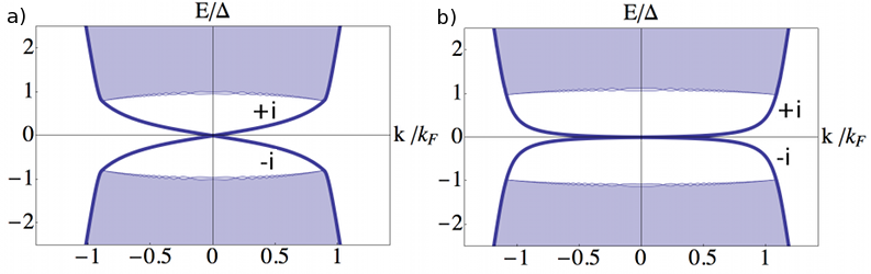
Figure 5: SABS dispersion for the tight-binding model in which a) $m=0.3>0$, $\mu_{1}=0.6$ corresponds to a doped BI; b) $m=0$, $\mu_{1}=0.6$ corresponds to a doped zero-gap semiconductor.

I.4 IV. Relation to Previous Works

In a recent work, Hao and Leehaolee calculated the surface spectral function in tight-binding models for Cu_xBi₂Se₃ with the four possible pairing symmetriesfuberg , including the fully-gapped odd-parity pairing studied in this work. They used two tight-binding models which are lattice regularizations of two $k\cdot p$ Hamiltonians (I and II). However, both these Hamiltonians violate the mirror symmetry. Model II is quoted from the incorrect $k\cdot p$ Hamiltonian of Ref.zhang : their terms $k_{z}\sigma_{x}s_{z}$ as well as $\sigma_{x}(k_{x}s_{x}+k_{y}s_{y})$, in the basis they specify, violates the mirror symmetry $M$. A corrected versionliu is identical to our $k\cdot p$ Hamiltonian (1) after interchanging $\sigma_{x}$ and $\sigma_{z}$ (corresponding to a change of basis for the orbitals). Model I is claimed to be quoted from Ref.fuberg (the one we use here). However, the term $\sigma_{z}(k_{x}s_{y}-k_{y}s_{x})$ is mistakenly replaced by $\sigma_{z}(k_{x}s_{x}+k_{y}s_{y})$.

Nonetheless, if one forgoes the definition of $s_{x,y}$ as operators corresponding to spin along the x and y directions in real space, then their Model I corresponds to our $k\cdot p$ Hamiltonian after a unitary spin rotation $\exp(-i\frac{\pi}{4}s_{z})$ (without affecting the odd-parity pairing term $\Delta\sigma_{y}s_{z}\tau_{x}$). Hence, they also found that Majorana fermion Andreev bound states at $k=0$ connect to the Dirac surface states near Fermi momentum. They attributed the second crossing to the fact that Dirac surface states remain gapless in the odd-parity superconducting state, and concluded that it disappears if the surface states merge into the bulk. In contrast, our work revealed the topological origin of the twisted surface Andreev bound states: as long as $\tilde{v}/v<0$, they are protected by mirror symmetry and exist independent of whether Dirac surface states appear at Fermi energy.

I.5 V. Finite Temperature Differential Conductance

Finally, we elaborate on how we attained the differential conductance plots in the main text. Consider two systems separated by an insulating barrier. Then the tunneling current is proportional to the transition rate given by Fermi’s golden rule:

$$I\propto\int d\epsilon A^{+}_{1}(\epsilon+eV)A^{-}_{2}(\epsilon)-A^{-}_{1}(\epsilon+eV)A^{+}_{2}(\epsilon)$$ (42)

where $A^{+}(\epsilon)$ is the probability of adding a particle and changing the system’s energy by $\epsilon$ (positive or negative), and $A^{-}(\epsilon)$ is the probability of removing a particle and changing the system’s energy by $-\epsilon$. $1$ and $2$ denote the two sides of the barrier.

For free electron systems, $A^{\pm}$ is given by the density of states weighted by the Fermi-Dirac distribution

$$A^{\pm}(\epsilon) = \int dkA^{\pm}(\epsilon,k)$$

$$A^{-}(\epsilon,k) = n_{F}(\epsilon)\delta(\epsilon-\xi_{k})$$

$$A^{+}(\epsilon,k) = (1-n_{F}(\epsilon))\delta(\epsilon-\xi_{k})$$ (43)

where $n_{F}(\epsilon)$ is the Fermi-Dirac distribution function $1/(e^{\epsilon/T}+1)$. For convenience, hereafter both $\epsilon$ and $\xi_{k}$ are measured with respect to chemical potential.

For a BCS superconductor, $A^{\pm}$ is modified:

$$A^{-}(\omega,k) = |u_{k}|^{2}n_{F}(\omega)\delta(\omega-|\xi_{k}|),\;\omega>0$$

$$|v_{k}|^{2}(1-n_{F}(|\omega|))\delta(|\omega|-|\xi_{k}|),\;\omega<0$$

$$A^{+}(\omega,k) = |u_{k}|^{2}(1-n_{F}(\omega))\delta(\omega-|\xi_{k}|),\;\omega>0$$ (44)

$$|v_{k}|^{2}n_{F}(|\omega|)\delta(|\omega|-|\xi_{k}|),\;\omega<0$$

where $|\xi_{k}|>0$ is the energy cost of creating a quasi-particle excitation. $u$ and $v$ are the particle and hole components of the positive-energy eigenstates of BdG Hamiltonian, respectively. To derive (45), one must keep in mind that adding(removing) a quasi-particle always increases(decreases) the energy of the system. Because the hole component of a $E>0$ eigenstate is related to the particle component of its partner at $-E$ by the inherent particle-hole symmetry in BdG formalism, (45) can be simplified to

$$A^{-}(\omega,k) = |u_{k}|^{2}n_{F}(\omega)\delta(\omega-\xi_{k}),$$

$$A^{+}(\omega,k) = |u_{k}|^{2}(1-n_{F}(\omega))\delta(\omega-\xi_{k}),$$ (45)

where we have used $1-n_{F}(-\omega)=n_{F}(\omega)$. Here $\omega$ and $\xi_{k}$ can be both positive and negative. Written in this form, $A^{\pm}$ for a superconductor is similar to a normal metal, except it has prefactor $u_{k}$. When superconductivity vanishes, $u_{k}=1,v_{k}=0$ for $k>k_{F},\omega>0$ and $k<k_{F},\omega<0$, whereas $u_{k}=0,v_{k}=1$ for $k<k_{F},\omega>0$ and $k>k_{F},\omega<0$. In this limit, (45) reduces to the free fermion case (43).

In our simulation, $|u_{k}|^{2}$ and $|v_{k}|^{2}$ were obtained from the $\tau=1$ and $\tau=-1$ components of the surface Green’s function, summed over spin and for the $\sigma_{z}=+1$ orbital at $z=0$ only, in accordance with our boundary condition. The surface Green’s function was computed using a recursive algorithm greens , allowing us to use a very large slab size ($2^{24}$ layers).

Substituting $A^{\pm}$ into the expression for tunneling current and assuming that the density of states of the normal metal is constant, we obtain

$$I \propto \int_{-\infty}^{\infty}d\epsilon\rho_{N}\rho_{S}(\omega)[n_{F}(\omega-eV)-n_{F}(\omega)],$$ (46)

Differentiating $I$ with respect to $V$ gives the differential conductance

$$dI/dV \propto \int_{-\infty}^{\infty}d\epsilon\rho_{S}(\omega)(dn_{F}/d\omega)|_{\omega-eV}$$

$$\rho_{S}(\omega) = \int dk|u_{k}|^{2}\delta(\omega-\xi_{k}).$$ (47)

References

- (1) S. Sasaki et. al., arXiv:1108.1101
- (2) A. Schynder, S. Ryu, A. Furusaki and A. Ludwig, Phys. Rev. B 78, 195125 (2008).
- (3) A. Kitaev, arXiv:0901.2686
- (4) N. Read and D. Green, Phys. Rev. B 61, 10267 (2000).
- (5) R. Roy, arXiv:0803.2868
- (6) X. L. Qi, T. L. Hughes, S. C. Zhang, Phys. Rev.Lett. 102, 187001 (2009)
- (7) M. M. Salomaa and G. E. Volovik, Phys. Rev. B 37, 9298 (1988); M. A. Silaev, G. E. Volovik, J. Low Temp. Phys., 161, 460 (2010).
- (8) S. K. Yip, J. Low Temp. Phys., 160, 12 (2010).
- (9) S. Ryu, J. E. Moore and A. Ludwig, arXiv:1010.0936
- (10) K. Nomura, S. Ryu, A. Furusaki, and N. Nagaosa, arXiv:1108.5054
- (11) L. Fu and E. Berg, Phys. Rev. Lett. 105, 097001 (2010).
- (12) X. L. Qi, T. L. Hughes, S. C. Zhang, Phys. Rev. B 81, 134508 (2010).
- (13) M. Sato, Phys. Rev. B 81, 220504(R) (2010).
- (14) Y. Hor et al, Phys. Rev. Lett. 104, 057001 (2010)
- (15) P. A. Lee, Journal Club for Condensed Matter Physics, Feb 2010: http://www.condmatjournalclub.org/?p=833
- (16) L. A. Wray et al, Nature Physics, 6, 855 (2010); Phys. Rev. B, 83, 224516 (2011).
- (17) M. Kriener et al, Phys. Rev. Lett. 106, 127004 (2011).
- (18) M. Kriener, et al, Phys. Rev. B 84, 054513 (2011).
- (19) P. Das et al, Phys. Rev. B 83, 220513(R) 2011).
- (20) L. Hao and T. K. Lee, Phys. Rev. B 83, 134516 (2011)
- (21) For reviews on surface Andreev bound states in unconventional superconductors, see S. Kashiwaya and Y. Tanaka, Rep. Prog. Phys. 63, 1641 (2000); G. Deutscher, Rev. Mod. Phys. 77, 109 (2005).
- (22) H. Zhang et al, Nature Phys. 5, 438 (2009).
- (23) C. X. Liu et al, Phys. Rev. B 82, 045122 (2010).
- (24) See Supplemental Material at […] for details.
- (25) J. C. Y. Teo, L. Fu, and C. L. Kane. Phys Rev. B, 78, 045426. (2008).
- (26) R. Takahashi and S. Murakami, arXiv:1105.5209
- (27) Strictly speaking, mirror helicity protects the second crossing along the mirror-invariant line only. However, higher order terms which reduce the full rotational symmetry are small.
- (28) L. Fu and C. L. Kane, Phys. Rev. B 76, 045302 (2007).
- (29) For a general discussion of boundary conditions for Dirac materials, see A. R. Akhmerov and C. W. J. Beenakker, Phys. Rev. B 77, 085423 (2008).
- (30) Y. Qi and L. Fu, to be published.
- (31) J. L. Zhang et al, PNAS, 108, 24 (2011).
- (32) R. A. Hein and E. M. Swiggard, Phys. Rev. Lett. 24, 53 (1970).
- (33) Y. Matsushita et al, Phys. Rev. B 74, 134512 (2006).
- (34) R. Hein, Physics Letters 23, 435 (1966).
- (35) R. A. Hein et al, Phys. Rev. Lett. 12, 320 (1964).
- (36) N. P. Butch et al, arXiv:1109.0979
- (37) T. Kirzhner et al, arXiv:1111.5805
- (38) Hsin Lin, private communication; Junwei Liu, private communication.
- (39) M. P. Lopez Sancho et al, J. Phys. F: Met. Phys. 15 (1985).