Wannier-based calculation of the orbital magnetization in crystals

Abstract

We present a first-principles scheme that allows the orbital magnetization of a magnetic crystal to be evaluated accurately and efficiently even in the presence of complex Fermi surfaces. Starting from an initial electronic-structure calculation with a coarse ab initio ${\bf k}$-point mesh, maximally localized Wannier functions are constructed and used to interpolate the necessary ${\bf k}$-space quantities on a fine mesh, in parallel to a previously-developed formalism for the anomalous Hall conductivity [X. Wang, J. Yates, I. Souza, and D. Vanderbilt, Phys. Rev. B 74, 195118 (2006)]. We formulate our new approach in a manifestly gauge-invariant manner, expressing the orbital magnetization in terms of traces over matrices in Wannier space. Since only a few (e.g., of the order of 20) Wannier functions are typically needed to describe the occupied and partially occupied bands, these Wannier matrices are small, which makes the interpolation itself very efficient. The method has been used to calculate the orbital magnetization of bcc Fe, hcp Co, and fcc Ni. Unlike an approximate calculation based on integrating orbital currents inside atomic spheres, our results nicely reproduce the experimentally measured ordering of the orbital magnetization in these three materials.

I Introduction

Magnetism in matter originates from two distinct sources, namely, the spin and the orbital degrees of freedom of the electrons. In many bulk ferromagnets the spin contribution dominates, and it is therefore not surprising that the description of spin magnetism using first-principles methods is considerably more developed than that of orbital magnetism. In particular, the local spin-density approximation has been successful in studying magnetic materials for decades.Martin_04

Although the orbital moments in bulk solids are strongly quenched by the crystal field and typically give small contributions to the net magnetization—between 5% and 10% in Fe, Co, and Ni—they can be measured very accurately with the help of gyromagnetic experiments.Meyer61 ; scott-rmp62 Moreover, there are known instances where orbital magnetism plays a prominent role. Some examples include weak ferromagnets with large but opposing spin and orbital moments,Qiao_04 ; Gotsis_03 ; Taylor_02 low-coordination systems such as magnetic nanowires,gambardella-nature02 and the recently-predicted large orbital magnetoelectric coupling in topological insulators and related materials.qi-prb08 ; essin-prl09 ; coh-prb11 In addition, magnetic resonance parameters such as the NMRCeresoli_10a ; Thonhauser_09a ; Thonhauser_09b and EPRCeresoli_10b shielding tensors can be conveniently calculated as the change in (orbital) magnetization under appropriate perturbations. These examples highlight the need to develop accurate and efficient first-principles schemes for describing orbital magnetism in solids.

The traditional way of computing the orbital magnetization ${\bf M}$ is by integrating currents inside atom-centered muffin-tin spheres.Wu_01 ; Sharma_07 This requires choosing, somewhat arbitrarily, a cutoff radius and neglects contributions from the interstitial regions. A rigorous theory for the orbital magnetization of periodic crystals free from such uncontrolled approximations was obtained only recentlyThonhauser05 ; Xiao05 ; Ceresoli06 ; Shi_07 (see Ref. Thonhauser_11, for a review). The theory was developed in the independent-particle framework, and its central result is the expression

$$\begin{split}{\bf M}&=\frac{e}{2\hbar}\;{\rm Im}\;\sum_{n}\int[dk]\;f_{n{\bf k}}\\ &\cdot\langle\partial_{\bf k}u_{n{\bf k}}|\times\big{(}\hat{H}_{\bf k}+\varepsilon_{n{\bf k}}-2\varepsilon_{F}\big{)}|\partial_{\bf k}u_{n{\bf k}}\rangle\;.\end{split}$$ (1)

Here the integral is over the Brillouin zone (BZ), $[dk]$ stands for $d{\bf k}/(2\pi)^{3}$, $\hat{H}_{\bf k}=e^{-i{\bf k}\cdot{\bf r}}\hat{\cal H}e^{i{\bf k}\cdot{\bf r}}$ is the Bloch Hamiltonian whose eigenfunctions are the cell-periodic Bloch functions $|u_{n{\bf k}}\rangle$ with eigenvalues $\varepsilon_{n{\bf k}}$, $f_{n{\bf k}}$ is the zero-temperature Fermi occupation factor, and $\varepsilon_{F}$ is the Fermi energy. The third term in Eq. (1) vanishes in ordinary insulators, but must be included in the case of metals.Xiao05 ; Ceresoli06 ; Shi_07

The implementation of Eq. (1) requires a knowledge of the ${\bf k}$-space gradients $|\partial_{\bf k}u_{n{\bf k}}\rangle$ of the occupied Bloch states.Thonhauser_11 An easier quantity to compute in practice is the covariant derivative $|\widetilde{\partial}_{\bf k}u_{n{\bf k}}\rangle$, defined as the projection of $|\partial_{\bf k}u_{n{\bf k}}\rangle$ onto the unoccupied bands. It turns out that the replacement $|\partial_{\bf k}u_{n{\bf k}}\rangle\rightarrow|\widetilde{\partial}_{\bf k}u_{n{\bf k}}\rangle$ in Eq. (1) leaves the sum of its terms invariant. For band insulators the covariant derivative can be conveniently evaluated by finite differences.Ceresoli06 Unfortunately, the discretized covariant derivative approach cannot be applied to metals, as it relies on having a constant number of occupied bands throughout the BZ.

Thus far, the only first-principles application of Eq. (1) to metals is the calculation in Ref. Ceresoli_10b, of the spontaneous orbital magnetization in Fe, Co, and Ni crystals, where the ${\bf k}$-derivatives of the Bloch wave functions were evaluated using a linear-response method.k.p This carries a cost per ${\bf k}$-point comparable to that of a non-self-consistent ground-state calculation. The number of ${\bf k}$-points needed to converge the BZ integral in Eq. (1) for Fe, Co, and Ni is quite significant, rendering the full calculation rather time-consuming.

In this work we develop an alternative approach which greatly reduces the computational cost of evaluating Eq. (1) for metals. Our implementation relies on a method for constructing well-localized crystalline Wannier functions (WFs) by post-processing a conventional band structure calculation.Marzari97 A key ingredient is the “band disentanglement” procedure of Ref. Souza01, , which allows one to obtain a set of WFs spanning a space that contains the occupied valence bands as a subspace. These WFs are essentially an exact tight-binding basis for those ab initio bands that carry the information about ${\bf M}$. Working in the Wannier representation, the problem of evaluating ${\bf M}$ can then be reformulated in a very economical way. This reformulation involves setting up the matrix elements of certain operators in the Wannier basis. Once that is done, the integrand of Eq. (1) can be evaluated very inexpensively and accurately at arbitrary points in the BZ. The cost per ${\bf k}$-point of the entire procedure is significantly reduced, especially in cases where a dense sampling of the BZ is needed to achieve convergence. Our method builds on the work of Ref. Wang06, , where a similar “Wannier interpolation” strategy was introduced to calculate the anomalous Hall conductivity (AHC) of ferromagnetic metals.

This manuscript is organized as follows. In Sec. II the orbital magnetization formula, Eq. (1), is recast in a gauge-invariant form, and a related expression for the AHC is introduced. We then describe step by step the formalism used to express physical quantities in the Wannier representation. That formalism is applied in Sec. III first to the AHC, and then to the orbital magnetization. In Sec. IV we describe the procedure for evaluating the required ${\bf k}$-space matrices by Fourier interpolation. Some details of the first-principles calculation and Wannier-function construction are given in Sec. V, followed by an application of the method to bcc Fe, hcp Co, and fcc Ni in Sec. VI. We conclude in Sec. VII with a brief summary and discussion.

II Preliminaries

II.1 Orbital magnetization and anomalous Hall conductivity

For our purposes it will be convenient to recast Eq. (1) in a different form as introduced in Ref. Ceresoli06, . We begin by writing the axial vector ${\bf M}$ as an antisymmetric tensor,

$$M_{\alpha\beta}=\frac{1}{2}\epsilon_{\alpha\beta\gamma}M_{\gamma}\;,$$ (2)

where Greek indices denote Cartesian directions. We now partition $M_{\alpha\beta}$ into two terms,

$$M_{\alpha\beta}=\widetilde{M}_{\alpha\beta}^{\rm LC}+\widetilde{M}_{\alpha\beta}^{\rm IC}\;.$$ (3)

The “local circulation” is

$$\widetilde{M}_{\alpha\beta}^{\rm LC}=-\frac{e}{2\hbar}\int[dk]\,\left[-2\,{\rm Im}(G_{\alpha\beta}-\varepsilon_{F}F_{\alpha\beta})\right],$$ (4)

and the “itinerant circulation” is

$$\widetilde{M}_{\alpha\beta}^{\rm IC}=-\frac{e}{2\hbar}\int[dk]\,\left[-2\,{\rm Im}(H_{\alpha\beta}-\varepsilon_{F}F_{\alpha\beta})\right].$$ (5)

The ${\bf k}$-dependent quantities $F_{\alpha\beta}$, $G_{\alpha\beta}$, and $H_{\alpha\beta}$ are

$$F_{\alpha\beta} = {\rm Tr}\left[(\partial_{\alpha}\hat{P})\hat{Q}(\partial_{\beta}\hat{P})\right]\;,$$ (6)

$$G_{\alpha\beta} = {\rm Tr}\left[(\partial_{\alpha}\hat{P})\hat{Q}\hat{H}\hat{Q}(\partial_{\beta}\hat{P})\right]\;,$$ (7)

$$H_{\alpha\beta} = {\rm Tr}\left[\hat{H}(\partial_{\alpha}\hat{P})\hat{Q}(\partial_{\beta}\hat{P})\right]\;,$$ (8)

where “Tr” denotes the electronic trace, $\partial_{\alpha}$ stands for $\partial/\partial k_{\alpha}$, and the subscript ${\bf k}$ is implied in the Bloch Hamiltonian $\hat{H}$ and in the projection operators $\hat{P}$ and $\hat{Q}=\hat{\mathbbm{1}}-\hat{P}$ spanning the occupied and unoccupied spaces respectively (here $\hat{\mathbbm{1}}$ is the identity operator in the full Hilbert space).

We work at $T=0$, so that Eqs. (2)–(8) yield the same result as Eq. (1). This can be seen by writing $\hat{P}$ in terms of the Bloch eigenstates,

$$\hat{P}=\sum_{n}\,|u_{n}\rangle f_{n}\langle u_{n}|$$ (9)

and setting the occupancies $f_{n}$ to either one or zero.

Compared to Eq. (1), the above formulation has the advantage of being manifestly gauge-invariant, i.e., independent of any ${\bf k}$-dependent phase twists applied to the occupied Bloch states, or more generally, any ${\bf k}$-dependent unitary mixing among them. Because Eqs. (6)–(8) are written as traces involving projection operators, they remain valid no matter how we choose to represent the occupied space at each ${\bf k}$. Instead, Eq. (1) is written explicitly in terms of the energy eigenstates, that is, it assumes a Hamiltonian gauge.

It should come as no surprise that it is possible to cast a physical observable such as the orbital magnetization in a gauge-invariant form. More interestingly, the two terms in Eq. (3) are individually gauge-invariant, and this led to the speculation that they might be separately observable.Ceresoli06 That is indeed the case—at least in principle—as discussed in Ref. Souza08, .

Before continuing we mention another physical observable, the intrinsic anomalous Hall conductivity, which can be expressed in gauge-invariant form as

$$\sigma_{\alpha\beta}^{\rm AH}=-\frac{e^{2}}{\hbar}\int[dk]\,\left(-2\,{\rm Im}\,F_{\alpha\beta}\right)\;.$$ (10)

In the Hamiltonian gauge the integrand of this equation acquires a more familiar form, i.e., as the ${\bf k}$-space Berry curvature summed over the occupied bands.Ceresoli06

While developing the formalism in Sec. III we shall first consider the AHC before tackling the more complex case of the orbital magnetization. This will allow us to make contact with the work of Ref. Wang06, , where a Wannier interpolation scheme was developed for the AHC, but using a somewhat different formulation.

II.2 Wannier space and gauge freedom

The crux of our approach is to express the observables of interest (orbital magnetization and AHC) not in terms of the Bloch eigenstates $|u_{n{\bf k}}\rangle$, but using an alternative set of Bloch-like states $|u^{{\rm W}}_{n{\bf k}}\rangle$ constructed at each ${\bf k}$ as appropriately chosen linear combinations of energy eigenstates. The defining feature of the new states is that they are smooth functions of ${\bf k}$. As a result, the corresponding Wannier functions (WFs)

$$|{\bf R}n\rangle=\frac{1}{{\cal N}^{3}}\sum_{\bf k}\,e^{-i{\bf k}\cdot({\bf R}-{\bf r})}|u^{{\rm W}}_{n{\bf k}}\rangle$$ (11)

(here ${\cal N}^{3}$ is the number of ${\bf k}$-points distributed on a uniform BZ mesh) are well-localized in real space, and for this reason we shall say that the states $|u^{{\rm W}}_{n{\bf k}}\rangle$ belong to the Wannier gauge. The ability to construct a short-ranged representation of the electronic structure in real space is what will allow us to devise an efficient and accurate interpolation scheme for the ${\bf k}$-space quantities ${\rm Im}\,F_{\alpha\beta}$, ${\rm Im}\,G_{\alpha\beta}$, and ${\rm Im}\,H_{\alpha\beta}$.

The construction of a Wannier basis proceeds in two steps, which we call “space selection” and “gauge selection.” In the case of insulators, the space selection is typically obvious; we want the WFs to span just the occupied subspace. In ${\bf k}$-space, we represent this subspace by a ${\bf k}$-dependent “band projection operator” $\hat{P}_{\bf k}$ defined as in Eq. (9) (with $f_{n}=1$ and 0 for occupied and empty bands respectively). Denoting the Wannier-space projection operator by $\hat{\mathbbm{P}}_{\bf k}$, we can then set $\hat{\mathbbm{P}}_{\bf k}=\hat{P}_{\bf k}$.

For metals, on the other hand, the space selection step, also known as “band disentanglement,” is more subtle. One wants to choose a $J$-dimensional manifold, represented by the projection operator $\hat{\mathbbm{P}}_{\bf k}$, throughout the BZ such that it has the following properties: (i) it must contain as a subspace the set of all occupied eigenstates (hence $J$ cannot be less than the highest number of occupied bands at any ${\bf k}$); (ii) it must display a smooth variation with ${\bf k}$, in the sense that $\hat{\mathbbm{P}}_{\bf k}$ is a differentiable function of ${\bf k}$. A procedure for extracting an optimally-smooth space from a larger set of band states was developed in Ref. Souza01, . The resulting space typically contains some admixture of low-lying empty states in addition to the occupied states.

The gauge selection consists of representing the smoothly-varying space $\hat{\mathbbm{P}}_{\bf k}$ using a set of $J$ Bloch-like states which are themselves smooth functions of ${\bf k}$,

$$\hat{\mathbbm{P}}_{\bf k}=\sum_{n}^{J}\,|u^{{\rm W}}_{n{\bf k}}\rangle\langle u^{{\rm W}}_{n{\bf k}}|\;.$$ (12)

From these $|u^{{\rm W}}_{n{\bf k}}\rangle$ the WFs are constructed via Eq. (11). A procedure for selecting an optimally-smooth Wannier gauge was developed in Ref. Marzari97, , such that the resulting WFs are maximally-localized in the sense of having the smallest possible quadratic spread. The localization procedure was originally devised with an isolated group of bands in mind (e.g., the valence bands of an insulator), but it can be applied to any smoothly-varying Bloch manifold of fixed dimension $J$.

In the Wannier gauge the projected Hamiltonian $\hat{\mathbbm{H}}_{\bf k}=\hat{\mathbbm{P}}_{\bf k}\hat{H}_{\bf k}\hat{\mathbbm{P}}_{\bf k}$ takes the form of a non-diagonal $J\times J$ matrix,

$$\mathbbm{H}^{{\rm W}}_{nm}({\bf k})=\langle u^{{\rm W}}_{n{\bf k}}|\hat{H}_{\bf k}|u^{{\rm W}}_{m{\bf k}}\rangle\;.$$ (13)

We define the Hamiltonian gauge in the projected space as the gauge in which this matrix becomes diagonal,

$$\mathbbm{H}_{nm}^{{\rm H}}({\bf k})=U^{\dagger}({\bf k})\mathbbm{H}^{{\rm W}}({\bf k})U({\bf k})=\overline{\varepsilon}_{n{\bf k}}\delta_{nm}\;.$$ (14)

Because of the nature of the space selection step, the “projected eigenvalues” $\overline{\varepsilon}_{n{\bf k}}$ agree with the true ab initio eigenvalues $\varepsilon_{n{\bf k}}$ for all occupied states, but they may differ for unoccupied states.

The unitary matrices $U({\bf k})$ that diagonalize $\mathbbm{H}^{{\rm W}}({\bf k})$ can be used to transform other objects between the Wannier and Hamiltonian gauges. For example, the Bloch states transform as

$$|u^{{\rm H}}_{n{\bf k}}\rangle=\sum_{m}^{J}\,|u^{{\rm W}}_{m{\bf k}}\rangle U_{mn}({\bf k})\;.$$ (15)

The gauge-invariance of the projection operators $\hat{\mathbbm{P}}_{\bf k}$ can be checked explicitly by inserting the right-hand-side of Eq. (15) in place of $|u^{{\rm W}}_{n{\bf k}}\rangle$ in Eq. (12).

II.3 Projection operators and occupation matrices

Figure 1: The Hilbert space of Bloch functions at wavevector ${\bf k}$ can be decomposed either as $\hat{\mathbbm{1}}=\hat{P}+\hat{Q}$ (occupied and unoccupied spaces) or as $\hat{\mathbbm{1}}=\hat{\mathbbm{P}}+\hat{\mathbbm{Q}}$ (“inner” and “outer” spaces, where the “inner” space is spanned by Wannier functions).

In Eq. (9) we introduced the projection operator $\hat{P}_{\bf k}$ onto the occupied manifold at ${\bf k}$, and in Eq. (12) the projection operator $\hat{\mathbbm{P}}_{\bf k}$ onto the Wannier space at ${\bf k}$. Figure 1 represents schematically the relationship between those two subspaces, as well as other related subspaces to be defined shortly. The notation in the figure is as follows: a double staff is used for objects that concern the distinction between the space spanned by the WFs (“inner”) and the corresponding orthogonal space (“outer”), while a single staff will be used for objects that distinguish between the occupied and unoccupied parts of the Wannier space.

Consider, for example, the projection operator $\hat{P}$ onto the occupied bands, as defined in Eq. (9). Recall that ${\bf k}$ labels were suppressed in Sec II.1; with ${\bf k}$ temporarily restored, we have

$$\begin{split}\hat{P}_{\bf k}&=\sum_{n}^{J}|u^{{\rm H}}_{n{\bf k}}\rangle\,f^{{\rm H}}_{n{\bf k}}\,\langle u^{{\rm H}}_{n{\bf k}}|\\ &=\sum_{mn}^{J}|u^{{\rm W}}_{m{\bf k}}\rangle\,f^{{\rm W}}_{mn,{\bf k}}\,\langle u^{{\rm W}}_{n{\bf k}}|\;,\end{split}$$ (16)

where $f^{{\rm W}}_{mn,{\bf k}}=\langle u^{{\rm W}}_{m{\bf k}}|\hat{P}_{\bf k}|u^{{\rm W}}_{n{\bf k}}\rangle$ is the (non-diagonal) occupation matrix in the Wannier gauge. In the following, we will use a strongly condensed notation, leaving band indices (and sums over them) implicit, omitting wavevector subscripts, and dropping the superscript “W” from objects in the Wannier gauge. So, for example, we will write the Wannier-gauge Bloch states simply as $|u\rangle$ instead of $|u^{{\rm W}}_{n{\bf k}}\rangle$.

In this notation, $\hat{P}_{\bf k}$ is expressed in the Wannier gauge as just

$$\hat{P}=|u\rangle f\langle u|\;.$$ (17)

Similarly, the projector onto the Wannier (“inner”) space is

$$\hat{\mathbbm{P}}=|u\rangle\langle u|\;.$$ (18)

We also define

$$\hat{\mathbbm{Q}} = \hat{\mathbbm{1}}-\hat{\mathbbm{P}}\;,$$ (19)

$$\hat{Q} = \hat{\mathbbm{1}}-\hat{P}=\hat{Q}_{\rm in}+\hat{\mathbbm{Q}}\;,$$ (20)

with

$$\hat{Q}_{\rm in} = |u\rangle g\langle u|\;,$$ (21)

$$g = 1-f\;,$$ (22)

where “1” denotes the $J\times J$ identity matrix.

In practice the occupation matrix is first evaluated in the Hamiltonian gauge in which it is diagonal, and then rotated to the Wannier gauge with the help of Eq. (15),

$$f=Uf^{{\rm H}}U^{\dagger}\;.$$ (23)

The matrices $f$ and $g$ are idempotent, and satisfy

$$fg=gf=0\;,$$ (24)

as well as

$$[f,\mathbbm{H}]=[g,\mathbbm{H}]=0\;,$$ (25)

where

$$\mathbbm{H}=\langle u|\hat{H}|u\rangle$$ (26)

is Eq. (13) using the concise notation. Equations (24) and (25) imply

$$f\mathbbm{H}g=0\;.$$ (27)

Note that $f\mathbbm{H}=\mathbbm{H}f=f\mathbbm{H}f$. We shall also make frequent use of relations such as $\hat{Q}_{\rm in}\hat{\mathbbm{Q}}=\hat{\mathbbm{Q}}Q_{\rm in}=0$, $\hat{\mathbbm{Q}}^{2}=\hat{\mathbbm{Q}}$, $\hat{Q}_{\rm in}^{2}=\hat{Q}_{\rm in}$, etc.

II.4 Compendium of “geometric” matrix objects

We list here for future reference a number of additional $J\times J$ matrices that will be used to express ${\rm Im}\,F_{\alpha\beta}$, ${\rm Im}\,G_{\alpha\beta}$, and ${\rm Im}\,H_{\alpha\beta}$ in the Wannier representation:

$$\mathbbm{A}_{\alpha} = i\langle u|\partial_{\alpha}u\rangle\;,$$ (28)

$$\mathbbm{F}_{\alpha\beta} = \langle\partial_{\alpha}u|\partial_{\beta}u\rangle\;,$$ (29)

$$\widetilde{\mathbbm{F}}_{\alpha\beta} = \langle\partial_{\alpha}u|\hat{\mathbbm{Q}}|\partial_{\beta}u\rangle=\mathbbm{F}_{\alpha\beta}-\mathbbm{A}_{\alpha}\mathbbm{A}_{\beta}\;,$$ (30)

$$\mathbb{\Omega}_{\alpha\beta} = i\mathbbm{F}_{\alpha\beta}-i\mathbbm{F}_{\alpha\beta}^{\dagger}=\partial_{\alpha}\mathbbm{A}_{\beta}-\partial_{\beta}\mathbbm{A}_{\alpha}\;,$$ (31)

$$\widetilde{\mathbb{\Omega}}_{\alpha\beta} = i\widetilde{\mathbbm{F}}_{\alpha\beta}-i\widetilde{\mathbbm{F}}_{\alpha\beta}^{\dagger}=\mathbb{\Omega}_{\alpha\beta}-i\left[\mathbbm{A}_{\alpha},\mathbbm{A}_{\beta}\right]\;.$$ (32)

The Hermitian matrices $\mathbbm{A}_{\alpha}$, $\mathbb{\Omega}_{\alpha\beta}$, and $\widetilde{\mathbb{\Omega}}_{\alpha\beta}$ are known as the Berry connection, Berry curvature, and gauge-covariant Berry curvature. They play a central role in the theory of geometric-phase effects in solids.Xiao10

In addition to the above objects, which represent intrinsic properties of the Bloch manifold, we shall make use of a number of similarly-defined quantities which also depend on the Hamiltonian (and therefore are not strictly speaking “geometric”):

$$\mathbbm{B}_{\alpha} = i\langle u|\hat{H}|\partial_{\alpha}u\rangle\;,$$ (33)

$$\widetilde{\mathbbm{B}}_{\alpha} = i\langle u|\hat{H}\hat{\mathbbm{Q}}|\partial_{\alpha}u\rangle=\mathbbm{B}_{\alpha}-\mathbbm{H}\mathbbm{A}_{\alpha}\;,$$ (34)

$$\mathbbm{C}_{\alpha\beta} = \langle\partial_{\alpha}u|\hat{H}|\partial_{\beta}u\rangle\;,$$ (35)

$$\widetilde{\mathbbm{C}}_{\alpha\beta} = \langle\partial_{\alpha}u|\hat{\mathbbm{Q}}\hat{H}\hat{\mathbbm{Q}}|\partial_{\beta}u\rangle$$ (36)

$$= \mathbbm{C}_{\alpha\beta}-\mathbbm{A}_{\alpha}\widetilde{\mathbbm{B}}_{\beta}-\mathbbm{B}^{\dagger}_{\alpha}\mathbbm{A}_{\beta}\;,$$

$$\mathbb{\Lambda}_{\alpha\beta} = i\mathbbm{C}_{\alpha\beta}-i\mathbbm{C}^{\dagger}_{\alpha\beta}\;,$$ (37)

$$\widetilde{\mathbb{\Lambda}}_{\alpha\beta} = i\widetilde{\mathbbm{C}}_{\alpha\beta}-i\widetilde{\mathbbm{C}}^{\dagger}_{\alpha\beta}$$ (38)

$$= \mathbb{\Lambda}_{\alpha\beta}-i\left(\mathbbm{A}_{\alpha}\widetilde{\mathbbm{B}}_{\beta}-\mathbbm{A}_{\beta}\mathbbm{B}_{\alpha}-\text{h.c.}\right),$$

where “h.c.” stands for Hermitian conjugate. Note that while $\mathbb{\Lambda}_{\alpha\beta}$ and $\widetilde{\mathbb{\Lambda}}_{\alpha\beta}$ are Hermitian, $\mathbbm{B}_{\alpha}$ is not.

All of the matrices listed above are written in the Wannier gauge, where they are smooth functions of ${\bf k}$ and can be evaluated efficiently using Fourier transforms, as will be described in Sec. IV.

III Wannier-space representation of physical quantities

III.1 Anomalous Hall conductivity

III.1.1 Derivation

As a first application of our formalism, let us consider Eq. (10) for the AHC. The integrand is the Berry curvature $-2\,{\rm Im}\,F_{\alpha\beta}$, and we wish to write it as a trace of products of matrices defined within the Wannier space.

Our starting point is Eq. (6) for $F_{\alpha\beta}$. In preparation for taking the trace therein, let us express $(\partial_{\alpha}\hat{P})\hat{Q}$ in the Wannier gauge. Differentiating Eq. (17) leads to

$$\partial_{\alpha}\hat{P}=|\partial_{\alpha}u\rangle f\langle u|+|u\rangle f\langle\partial_{\alpha}u|+|u\rangle f_{\alpha}\langle u|\;,$$ (39)

where $f_{\alpha}=\partial_{\alpha}f$. Multiplying on the right with $\hat{Q}$ and using Eq. (20) yields two terms for $(\partial_{\alpha}\hat{P})\hat{Q}$. One is

$$(\partial_{\alpha}\hat{P})\hat{\mathbbm{Q}}=|u\rangle f\langle\partial_{\alpha}u|\hat{\mathbbm{Q}}\;,$$ (40)

where $\langle u|\hat{\mathbbm{Q}}=0$ was used, and the other is

$$(\partial_{\alpha}\hat{P})\hat{Q}_{\rm in}=|u\rangle f(+i\mathbbm{A}_{\alpha})g\langle u|+|u\rangle f_{\alpha}g\langle u|\;,$$ (41)

where Eq. (24) was used. Now, from Eq. (23) we findfootnote1

$$f_{\alpha}=i\left[f,J_{\alpha}\right]\;,$$ (42)

where the Hermitian matrix $J_{\alpha}$, like $f$ itself, is first evaluated in the Hamiltonian gauge, being defined as

$$J_{\alpha}^{{\rm H}}=iU^{\dagger}\partial_{\alpha}U\;,$$ (43)

and then rotated into the Wannier gauge,

$$J_{\alpha}=UJ_{\alpha}^{{\rm H}}U^{\dagger}\;.$$ (44)

Using Eq. (42) in Eq. (41) and defining

$$A_{\alpha}=\mathbbm{A}_{\alpha}+J_{\alpha}\;,$$ (45)

we arrive at the compact form

$$(\partial_{\alpha}\hat{P})\hat{Q}_{\rm in}=i|u\rangle fA_{\alpha}g\langle u|\;.$$ (46)

The desired expression is the sum of Eqs. (40) and (46),

$$(\partial_{\alpha}\hat{P})\hat{Q}=|u\rangle f\langle\partial_{\alpha}u|\hat{\mathbbm{Q}}+i|u\rangle fA_{\alpha}g\langle u|\;.$$ (47)

With this relation in hand it becomes straightforward to evaluate Eq. (6), and we quickly arrive at

$$F_{\alpha\beta}={\rm tr}\left[f\widetilde{\mathbbm{F}}_{\alpha\beta}+fA_{\alpha}gA_{\beta}\right],$$ (48)

where “tr” denotes the trace over $J\times J$ matrices, not to be confused with the trace “Tr” over the full Hilbert space introduced earlier. We are interested in the imaginary part, and using Eq. (32) we find

$$-2\,{\rm Im}\,F_{\alpha\beta} = {\rm Re}\,{\rm tr}[f\widetilde{\mathbb{\Omega}}_{\alpha\beta}]-2\,{\rm Im}\,{\rm tr}[fA_{\alpha}gA_{\beta}]$$

$$= {\rm Re}\,{\rm tr}[f\mathbb{\Omega}_{\alpha\beta}]+2\,{\rm Im}\,{\rm tr}[f\mathbbm{A}_{\alpha}\mathbbm{A}_{\beta}-fA_{\alpha}gA_{\beta}]\;.$$

Expanding $A_{\alpha}$ and using the identity

$${\rm Im}\,{\rm tr}[f\mathbbm{A}_{\alpha}\mathbbm{A}_{\beta}] = {\rm Im}\,{\rm tr}[f\mathbbm{A}_{\alpha}(f+g)\mathbbm{A}_{\beta}]$$

$$= {\rm Im}\,{\rm tr}[f\mathbbm{A}_{\alpha}g\mathbbm{A}_{\beta}]\;,$$

we end up with

$$-2\,{\rm Im}\,F_{\alpha\beta} = {\rm Re}\,{\rm tr}\left[f\mathbb{\Omega}_{\alpha\beta}\right]$$

$$- 2\,{\rm Im}\,{\rm tr}[f\mathbbm{A}_{\alpha}gJ_{\beta}+fJ_{\alpha}g\mathbbm{A}_{\beta}+fJ_{\alpha}gJ_{\beta}]\;.$$

This expression for the Berry curvature of the occupied states is our first important result.

III.1.2 Discussion

The ingredients that go into Eq. (III.1.1) are the matrices $\mathbbm{A}_{\alpha}$, $\mathbb{\Omega}_{\alpha\beta}$, $f$, and $J_{\alpha}$ expressed in a smooth (but otherwise arbitrary) gauge. It should be noted that while $\mathbbm{A}_{\alpha}$ and $\mathbb{\Omega}_{\alpha\beta}$ are themselves smooth functions of ${\bf k}$, this is not so for $f$ and $J_{\alpha}$. Consider $f$, given by Eq. (23). In metals it is affected by the step-like discontinuity in $f^{{\rm H}}$ at the Fermi surface. More generally it is also affected by the wrinkles in the rotation matrix $U$ (recall that $U$ relates via Eq. (15) the smooth Wannier-gauge Bloch states to the Hamiltonian-gauge states, which are non-analytic as a function of ${\bf k}$ at points of degeneracy). The situation is even more severe in the case of $J_{\alpha}$. Because it contains the derivative $\partial_{\alpha}U$ of a non-smooth function, it has spikes in ${\bf k}$-space.

How does one reconcile the existence of irregular and spiky quantities inside Eq. (III.1.1) with the form of Eq. (6), which suggests that $F_{\alpha\beta}$ is a smooth function of ${\bf k}$, except possibly when crossing the Fermi surface (when a state comes in or out of the occupied manifold, introducing a discontinuity in $\hat{P}_{\bf k}$)? The answer is that while $J_{\alpha}$ itself has a very irregular behavior, combinations like $fJ_{\alpha}g$ which actually appear in Eq. (III.1.1) do not, as will be discussed in Sec. IV.1.

Let us now make contact with the formulation of Wannier interpolation developed in Ref. Wang06, . In that work the expression for the Berry curvature of the occupied states [Eq. (32) therein] was written in the Hamiltonian gauge, where the occupation matrices are diagonal. This required transforming $\mathbbm{A}_{\alpha}$ and $\mathbb{\Omega}_{\alpha\beta}$ from the Wannier gauge, where they are first constructed, to the Hamiltonian gauge. Here we choose to keep everything in the Wannier gauge throughout. The advantage is that even though the matrices $f$ and $J_{\alpha}$ have to be constructed first in the Hamiltonian gauge, it is straightforward to rotate them into the Wannier gauge where all other needed objects are constructed. Instead, the reverse transformation of those other objects can in certain cases become nontrivial.

The two formulations are of course equivalent, and it is instructive to recover explicitly from Eq. (III.1.1) the corresponding expression in Ref. Wang06, . Consider for example the last term in Eq. (III.1.1). Taking the trace in the Hamiltonian gauge we find

$${\rm tr}[fJ_{\alpha}gJ_{\beta}]=\sum_{nm}^{J}\,f_{n}^{{\rm H}}J^{{\rm H}}_{\alpha,nm}(1-f_{m}^{{\rm H}})J^{{\rm H}}_{\beta,mn}\;,$$ (52)

and thus

$$-2\,{\rm Im}\,{\rm tr}[fJ_{\alpha}gJ_{\beta}]=-i\sum_{nm}^{J}\,(f_{m}^{{\rm H}}-f_{n}^{{\rm H}})J^{{\rm H}}_{\alpha,nm}J^{{\rm H}}_{\beta,mn}\;,$$ (53)

which agrees with the last term in Eq. (32) of Ref. Wang06, ($D_{\alpha}^{({{\rm H}})}$ therein corresponds in our notation to $-iJ^{{\rm H}}_{\alpha}$).

It is pleasing to see that Eq. (III.1.1), when converted to the Hamiltonian gauge, reduces to what was termed in Ref. Wang06, the “sum over occupied bands” expression, where individual terms have spiky features only when two bands, one occupied the other empty, almost touch at the Fermi level, as the factor $f_{n}^{{\rm H}}-f_{m}^{{\rm H}}$ suppresses spikes associated with pairs of occupied states. As we shall see in Sec. IV.1, this is a general feature of our formulation, which leads naturally to expressions where the spiky object $J_{\alpha}$ appears under the trace sandwiched between $f$ and $g$.

III.2 Orbital magnetization

Let us now apply to ${\rm Im}\,H_{\alpha\beta}$ and ${\rm Im}\,G_{\alpha\beta}$ the same strategy developed above for ${\rm Im}\,F_{\alpha\beta}$, completing the list of quantities needed to evaluate the orbital magnetization. We remark that it would be possible to proceed along the lines of Ref. Wang06, in order to arrive at “sum over occupied bands” expressions for those quantities in the Hamiltonian gauge. However, we found such an approach to be rather cumbersome, especially in the case of ${\rm Im}\,G_{\alpha\beta}$.

III.2.1 Derivation

Inserting Eq. (47) into Eq. (8) leads to

$$H_{\alpha\beta}={\rm tr}\left[f\mathbbm{H}f\widetilde{\mathbbm{F}}_{\alpha\beta}+f\mathbbm{H}fA_{\alpha}gA_{\beta}\right],$$ (54)

so that

$$-2\,{\rm Im}\,H_{\alpha\beta} = {\rm Re}\,{\rm tr}\left[f\mathbbm{H}f\widetilde{\mathbb{\Omega}}_{\alpha\beta}\right]-2\,{\rm Im}\,{\rm tr}\left[f\mathbbm{H}fA_{\alpha}gA_{\beta}\right]$$ (55)

$$= {\rm Re}\,{\rm tr}\left[f\mathbbm{H}f\mathbb{\Omega}_{\alpha\beta}\right]$$

$$+ 2\,{\rm Im}\,{\rm tr}\left[f\mathbbm{H}f\mathbbm{A}_{\alpha}\mathbbm{A}_{\beta}-f\mathbbm{H}fA_{\alpha}gA_{\beta}\right].$$

Using Eq. (45), this takes the desired form

$$\begin{split}-2\,{\rm Im}\,H_{\alpha\beta}&={\rm Re}\,{\rm tr}\left[f\mathbbm{H}f\mathbb{\Omega}_{\alpha\beta}\right]+2\,{\rm Im}\,{\rm tr}\left[f\mathbbm{H}f\mathbbm{A}_{\alpha}f\mathbbm{A}_{\beta}\right]\\ &-2\,{\rm Im}\,{\rm tr}\left[f\mathbbm{H}f\left(\mathbbm{A}_{\alpha}gJ_{\beta}+J_{\alpha}g\mathbbm{A}_{\beta}+J_{\alpha}gJ_{\beta}\right)\right]\end{split}$$ (56)

in terms of basic matrix objects with every $J_{\alpha}$ sandwiched between an $f$ and a $g$ (after taking account of the cyclic property of the trace).

Repeating for $G_{\alpha\beta}$, we find

$$G_{\alpha\beta}={\rm tr}\left[f\left(\widetilde{\mathbbm{C}}_{\alpha\beta}+A_{\alpha}g\widetilde{\mathbbm{B}}_{\beta}+\widetilde{\mathbbm{B}}^{\dagger}_{\alpha}gA_{\beta}+A_{\alpha}g\mathbbm{H}gA_{\beta}\right)\right]$$ (57)

and

$$-2\,{\rm Im}\,G_{\alpha\beta}={\rm Re}\,{\rm tr}\left[f\widetilde{\mathbb{\Lambda}}_{\alpha\beta}\right]$$

$${}-2\,{\rm Im}\,{\rm tr}\left[\left(fA_{\alpha}g\widetilde{\mathbbm{B}}_{\beta}-\alpha\leftrightarrow\beta\right)+fA_{\alpha}g\mathbbm{H}gA_{\beta}\right]\;.$$

Expanding $\widetilde{\mathbb{\Lambda}}_{\alpha\beta}$ and $\widetilde{\mathbbm{B}}_{\beta}$, this becomes

$$-2\,{\rm Im}\,G_{\alpha\beta}={\rm Re}\,{\rm tr}\left[f\mathbb{\Lambda}_{\alpha\beta}\right]$$ (59)

$${}-2\,{\rm Im}\,{\rm tr}\Big{[}f\left(A_{\alpha}g\mathbbm{B}_{\beta}-A_{\alpha}g\mathbbm{H}\mathbbm{A}_{\beta}-\mathbbm{A}_{\alpha}\mathbbm{B}_{\beta}-\alpha\leftrightarrow\beta\right)$$

$${}+f\left(\mathbbm{A}_{\alpha}\mathbbm{H}\mathbbm{A}_{\beta}+A_{\alpha}g\mathbbm{H}gA_{\beta}\right)\Big{]}\;.$$

Next we expand $A_{\alpha}$ and gather terms in three groups, containing zero, one, and two occurrences of the matrices $J_{\alpha}$ and $J_{\beta}$,footnote2

$$-2\,{\rm Im}\,G_{\alpha\beta}=J0+J1+J2\;.$$ (60)

The $J2$ group contains only one term,

$$J2=-2\,{\rm Im}\,{\rm tr}\left[fJ_{\alpha}g\mathbbm{H}gJ_{\beta}\right]\;.$$ (61)

The $J1$ group is

$$J1 = -2\,{\rm Im}\,{\rm tr}\left[fJ_{\alpha}g\left(\mathbbm{B}_{\beta}-\mathbbm{H}\mathbbm{A}_{\beta}+\mathbbm{H}g\mathbbm{A}_{\beta}\right)-\alpha\leftrightarrow\beta\right]$$ (62)

$$= -2\,{\rm Im}\,{\rm tr}\left[fJ_{\alpha}g\mathbbm{B}_{\beta}-\alpha\leftrightarrow\beta\right]\;,$$

where in the second equality we replaced one instance of $g$ with $1-f$ and then used Eq. (27). The $J0$ group reads, after combining certain terms and canceling out some others,

$$J0={\rm Re}\,{\rm tr}\left[f\mathbb{\Lambda}_{\alpha\beta}\right]$$

$${}+2\,{\rm Im}\,{\rm tr}\left[f\left(\mathbbm{A}_{\alpha}f\mathbbm{B}_{\beta}-\mathbbm{A}_{\beta}f\mathbbm{B}_{\alpha}-\mathbbm{A}_{\alpha}\mathbbm{H}f\mathbbm{A}_{\beta}\right)\right]\;.$$

This can be simplified further with the help of the following identity proven in the Appendix,

$${\rm tr}\left[f\mathbbm{A}_{\alpha}f\mathbbm{B}_{\beta}\right]={\rm tr}\left[f\mathbbm{A}_{\alpha}f\mathbbm{H}\mathbbm{A}_{\beta}\right]\;,$$ (64)

which leads to

$$J0={\rm Re}\,{\rm tr}\left[f\mathbb{\Lambda}_{\alpha\beta}\right]-2\,{\rm Im}\,{\rm tr}\left[f\mathbbm{H}f\mathbbm{A}_{\alpha}f\mathbbm{A}_{\beta}\right].$$ (65)

Collecting terms, we find

$$-2\,{\rm Im}\,G_{\alpha\beta} = {\rm Re}\,{\rm tr}\left[f\mathbb{\Lambda}_{\alpha\beta}\right]-2\,{\rm Im}\,{\rm tr}\left[f\mathbbm{H}f\mathbbm{A}_{\alpha}f\mathbbm{A}_{\beta}\right]$$

$$- 2\,{\rm Im}\,{\rm tr}\left[f\left(J_{\alpha}g\mathbbm{B}_{\beta}-\alpha\leftrightarrow\beta\right)+fJ_{\alpha}g\mathbbm{H}gJ_{\beta}\right]\;.$$

III.2.2 Final expressions

The quantities ${\rm Im}\,F_{\alpha\beta}$, ${\rm Im}\,G_{\alpha\beta}$, and ${\rm Im}\,H_{\alpha\beta}$ enter the orbital magnetization expression in the combinations ${\rm Im}(G_{\alpha\beta}-\varepsilon_{F}F_{\alpha\beta})$ and ${\rm Im}(H_{\alpha\beta}-\varepsilon_{F}F_{\alpha\beta})$. Using the condensed notations

$$X^{0} = fXf\;,$$ (67)

$$X^{1} = gXg\;,$$ (68)

$$X^{+} = gXf\;,$$ (69)

$$X^{-} = fXg\;,$$ (70)

in Eqs. (III.1.1), (56), and (III.2.1), we obtain for the integrand of $\widetilde{M}_{\alpha\beta}^{\rm IC}$, Eq. (5),

$$-2\,{\rm Im}(H_{\alpha\beta}-\varepsilon_{F}F_{\alpha\beta})=$$

$${}+{\rm Re}\,{\rm tr}\left[\left(\mathbbm{H}^{0}-\varepsilon_{F}\right)\mathbb{\Omega}^{0}_{\alpha\beta}\right]+2\,{\rm Im}\,{\rm tr}\left[\mathbbm{H}^{0}\mathbbm{A}^{0}_{\alpha}\mathbbm{A}^{0}_{\beta}\right]$$

$${}-2\,{\rm Im}\,{\rm tr}\left[\left(\mathbbm{H}^{0}-\varepsilon_{F}\right)\left(\mathbbm{A}^{-}_{\alpha}J^{+}_{\beta}+J^{-}_{\alpha}\mathbbm{A}^{+}_{\beta}+J^{-}_{\alpha}J^{+}_{\beta}\right)\right]\;,$$

and for the integrand of $\widetilde{M}_{\alpha\beta}^{\rm LC}$, Eq. (4),

$$-2\,{\rm Im}(G_{\alpha\beta}-\varepsilon_{F}F_{\alpha\beta})=$$

$${}+{\rm Re}\,{\rm tr}\left[\mathbb{\Lambda}^{0}_{\alpha\beta}-\varepsilon_{F}\mathbb{\Omega}^{0}_{\alpha\beta}\right]-2\,{\rm Im}\,{\rm tr}\left[\mathbbm{H}^{0}\mathbbm{A}^{0}_{\alpha}\mathbbm{A}^{0}_{\beta}\right]$$

$${}-2\,{\rm Im}\,{\rm tr}\Big{\{}\big{[}J^{-}_{\alpha}\big{(}\mathbbm{B}^{+}_{\beta}-\varepsilon_{F}\mathbbm{A}^{+}_{\beta}\big{)}-\alpha\leftrightarrow\beta\big{]}$$

$${}+J^{-}_{\alpha}(\mathbbm{H}^{1}-\varepsilon_{F})J^{+}_{\beta}\Big{\}}\;.$$

Note that the second terms in these two equations are equal and opposite. For the special case of an insulator with $f=1$ and $g=0$, only the first two terms are nonzero in each of Eqs. (III.2.2-III.2.2), and these expressions reduce to those derived in Ref. Ceresoli06, .

IV Interpolation of the Wannier-gauge matrices

We calculate the orbital magnetization by averaging Eqs. (III.2.2) and (III.2.2) over a sufficiently dense grid of ${\bf k}$-points in order to approximate the BZ integrals in Eqs. (4) and (5). At each ${\bf k}$ the matrices $f$, $J_{\alpha}$, $\mathbbm{H}$, $\mathbbm{A}_{\alpha}$, $\mathbbm{B}_{\alpha}$, $\mathbb{\Omega}_{\alpha\beta}$, and $\mathbb{\Lambda}_{\alpha\beta}$ are needed, and they are calculated by Fourier interpolation as follows.

IV.1 Fourier transform expressions

We start with the matrix $\mathbbm{H}$. Inverting Eq. (11),

$$|u\rangle=\sum_{\bf R}\,e^{-i{\bf k}\cdot({\bf r}-{\bf R})}|{\bf R}\rangle\;,$$ (73)

and inserting into Eq. (26) yields

$$\mathbbm{H}=\sum_{\bf R}\,e^{i{\bf k}\cdot{\bf R}}\langle{\bf 0}|\hat{\cal H}|{\bf R}\rangle\;.$$ (74)

We emphasize that any desired wavevector ${\bf k}$ can be plugged into this expression, allowing one to smoothly interpolate the matrix $\mathbbm{H}$ between the ${\cal N}^{3}$ ab initio grid points used in Eq. (11) to construct the WFs. Diagonalizing $\mathbbm{H}$ [Eq. (14)] and using the resulting rotation matrix $U$ and interpolated eigenvalues $\overline{\varepsilon}_{n}$ in Eq. (23) yields the occupation matrix $f$.

Next we consider the matrix $J_{\alpha}$. In practice it can be calculated by inserting $U$ into Eq. (44) and then usingWang06

$$J^{{\rm H}}_{\alpha,nm}=\begin{cases}\displaystyle\frac{i\left[U^{\dagger}\mathbbm{H}_{\alpha}U\right]_{nm}}{\overline{\varepsilon}_{m}-\overline{\varepsilon}_{n}}&\text{if $n\not=m$}\\ 0&\text{if $n=m$}\end{cases},$$ (75)

where $\mathbbm{H}_{\alpha}=\partial_{\alpha}\mathbbm{H}$ is obtained by differentiating Eq. (74). In the vicinity of band degeneracies and weak avoided crossings the denominator in Eq. (75) becomes small, leading to strong peaks in $J^{{\rm H}}_{\alpha,nm}$ as a function of ${\bf k}$. If both bands $n$ and $m$ are occupied, such peaks must eventually cancel out in the final expressions for the AHC and orbital magnetization, as discussed in Sec. III.1.2.

We can make such cancellations explicit from the outset by noting that $J_{\alpha}$ only appears in the combinations $J^{-}_{\alpha}=fJ_{\alpha}g$ and $J^{+}_{\alpha}=gJ_{\alpha}f$. Taking the former, for example, we find using Eqs. (23) and (44) that

$$J^{-}_{\alpha}=UJ_{\alpha}^{{\rm H}-}U^{\dagger}$$ (76)

where the matrix elements of $J^{{\rm H}-}_{\alpha}=f^{{\rm H}}J^{{\rm H}}_{\alpha}\left(1-f^{{\rm H}}\right)$ are

$$J^{{\rm H}-}_{\alpha,nm}=\begin{cases}\displaystyle\frac{i\left[U^{\dagger}\mathbbm{H}_{\alpha}U\right]_{nm}}{\overline{\varepsilon}_{m}-\overline{\varepsilon}_{n}}&\text{if $n$ occupied and $m$ empty,}\\ 0&\text{otherwise.}\end{cases}$$ (77)

$J^{{\rm H}+}_{\alpha,nm}$ is given by a similar expression, but with $m$ occupied and $n$ empty. Unlike Eq. (75), the expressions for $J^{{\rm H}-}$ and $J^{{\rm H}+}_{\alpha}$ are well behaved in that they will only show peaks when the direct gap is small and mixing between occupied and empty states is strong. By working directly with them, we avoid introducing any quantity that would react strongly to crossings among occupied states.

While $f$, $J_{\alpha}^{-}$ and $J_{\alpha}^{+}$ are first calculated in the Hamiltonian gauge and then converted to the Wannier gauge, the remaining quantities entering Eqs. (III.2.2) and (III.2.2) are most easily calculated directly in the Wannier gauge, in the same way as $\mathbbm{H}$. It is sufficient to consider the Wannier representation of the three basic quantities $\mathbbm{A}_{\alpha}$, $\mathbbm{B}_{\alpha}$, and $\mathbbm{C}_{\alpha\beta}$ introduced in Sec. II.4. Inserting Eq. (73) into the respective definitions we find

$$\mathbbm{A}_{\alpha} = \sum_{\bf R}\,e^{i{\bf k}\cdot{\bf R}}\langle{\bf 0}|\hat{r}_{\alpha}|{\bf R}\rangle\;,$$ (78)

$$\mathbbm{B}_{\alpha} = \sum_{\bf R}\,e^{i{\bf k}\cdot{\bf R}}\langle{\bf 0}|\hat{\cal H}(\hat{r}-R)_{\alpha}|{\bf R}\rangle\;,$$ (79)

$$\mathbbm{C}_{\alpha\beta} = \sum_{\bf R}\,e^{i{\bf k}\cdot{\bf R}}\langle{\bf 0}|\hat{r}_{\alpha}\hat{\cal H}(\hat{r}-R)_{\beta}|{\bf R}\rangle\;.$$ (80)

The expressions for $\mathbb{\Omega}_{\alpha\beta}$ and $\mathbb{\Lambda}_{\alpha\beta}$ are obtained by inserting Eq. (78) into Eq. (31) and Eq. (80) into Eq. (37), respectively.

It was shown in Ref. Wang06, that the computation of the AHC requires a knowledge of the Wannier matrix elements of $\hat{\cal H}$ and $\hat{{\bf r}}$. Inspection of the Fourier transform expression given above reveals that the bulk orbital magnetization requires in addition the matrix elements of $\hat{\cal H}\hat{{\bf r}}$ and $\hat{{\bf r}}\hat{\cal H}\hat{{\bf r}}$. This is more than might have been anticipated, given that the matrix elements of $\hat{{\bf r}}$ and $\hat{\cal H}\hat{{\bf r}}$ are not needed for calculating the orbital moment of finite samples under open boundary conditions, but it is the price to be paid for a formulation that extends also to the case of periodic boundary conditions.

IV.2 Evaluation of the real-space matrices

We shall follow the approach of Ref. Wang06, , whereby the needed real-space matrix elements are actually evaluated in reciprocal space. Inverting the Fourier sums in Eqs. (74), (78), (79), and (80), we find

$$\langle{\bf 0}|\hat{\cal H}|{\bf R}\rangle = \frac{1}{{\cal N}^{3}}\sum_{\bf k}\,e^{-i{\bf k}\cdot{\bf R}}\mathbbm{H}_{\bf k}\;,$$ (81)

$$\langle{\bf 0}|\hat{r}_{\alpha}|{\bf R}\rangle = \frac{i}{{\cal N}^{3}}\sum_{\bf k}\,e^{-i{\bf k}\cdot{\bf R}}\langle u_{\bf k}|\partial_{\alpha}u_{\bf k}\rangle$$ (82)

$$\simeq \frac{i}{{\cal N}^{3}}\sum_{{\bf k},{\bf b}}\,e^{-i{\bf k}\cdot{\bf R}}w_{b}b_{\alpha}\mathbbm{M}_{{\bf k}\;{\bf b}}\;,$$

$$\langle{\bf 0}|\hat{\cal H}(\hat{r}-R)_{\alpha}|{\bf R}\rangle = \frac{i}{{\cal N}^{3}}\sum_{\bf k}\,e^{-i{\bf k}\cdot{\bf R}}\langle u_{\bf k}|\hat{H}_{\bf k}|\partial_{\alpha}u_{\bf k}\rangle$$ (83)

$$\simeq \frac{i}{{\cal N}^{3}}\sum_{{\bf k},{\bf b}}\,e^{-i{\bf k}\cdot{\bf R}}w_{b}b_{\alpha}\mathbbm{H}_{{\bf k},{\bf b}}\;,$$

$$\langle{\bf 0}|\hat{r}_{\alpha}\hat{\cal H}(\hat{r}-R)_{\beta}|{\bf R}\rangle = \frac{1}{{\cal N}^{3}}\sum_{\bf k}\,e^{-i{\bf k}\cdot{\bf R}}\langle\partial_{\alpha}u_{\bf k}|\hat{H}_{\bf k}|\partial_{\beta}u_{\bf k}\rangle$$

$$\simeq\frac{1}{{\cal N}^{3}}\sum_{{\bf k},{\bf b}_{1},{\bf b}_{2}}\mspace{-35.0mu} e^{-i{\bf k}\cdot{\bf R}}w_{b_{1}}b_{1\alpha}w_{b_{2}}b_{2\beta}\mathbbm{H}_{{\bf k},{\bf b}_{1},{\bf b}_{2}}\;,$$

where the sums are over the ${\cal N}^{3}$ points in the uniform ab initio mesh. The second equalities in Eqs. (82)–(IV.2) follow from using a finite-difference expression for the derivatives of the smooth Bloch states,Marzari97

$$|\partial_{\alpha}u_{\bf k}\rangle=\sum_{\bf b}w_{b}b_{\alpha}|u_{{\bf k}+{\bf b}}\rangle+{\cal O}(b^{2})$$ (85)

($w_{b}$ are appropriately chosen weights, and the sum is over shells of vectors ${\bf b}$ connecting a point ${\bf k}$ on the ab initio grid to its neighbors), together with the definitions

$$\mathbbm{H}_{{\bf k},{\bf b}} = \langle u_{\bf k}|\hat{H}_{\bf k}|u_{{\bf k}+{\bf b}}\rangle\;,$$ (86)

$$\mathbbm{M}_{{\bf k},{\bf b}} = \langle u_{\bf k}|u_{{\bf k}+{\bf b}}\rangle\;,$$ (87)

$$\mathbbm{H}_{{\bf k},{\bf b}_{1},{\bf b}_{2}} = \langle u_{{\bf k}+{\bf b}_{1}}|\hat{H}_{\bf k}|u_{{\bf k}+{\bf b}_{2}}\rangle\;,$$ (88)

which complement Eq. (26) for $\mathbbm{H}_{\bf k}$, needed in Eq. (81). Writing the states $|u\rangle$ as linear combinations of the original ab initio eigenstates $|u^{0}\rangle$,

$$|u_{n{\bf k}}\rangle=\sum_{m}^{{\cal J}_{\bf k}}|u^{0}_{m{\bf k}}\rangle V_{{\bf k},mn}\;,$$ (89)

we arrive at the following expressions for the $J\times J$ matrices appearing in Eqs. (81)–(IV.2):

$$\mathbbm{H}_{\bf k} = V_{\bf k}^{\dagger}{\cal H}_{\bf k}V_{\bf k}\;,$$ (90)

$$\mathbbm{H}_{{\bf k},{\bf b}} = V_{\bf k}^{\dagger}{\cal H}_{\bf k}{\cal M}_{{\bf k},{\bf b}}V_{{\bf k}+{\bf b}}\;,$$ (91)

$$\mathbbm{M}_{{\bf k},{\bf b}} = V_{\bf k}^{\dagger}{\cal M}_{\bf k}V_{{\bf k}+{\bf b}}\;,$$ (92)

$$\mathbbm{H}_{{\bf k},{\bf b}_{1},{\bf b}_{2}} = V_{{\bf k}+{\bf b}_{1}}^{\dagger}{\cal H}_{{\bf k},{\bf b}_{1},{\bf b}_{2}}V_{{\bf k}+{\bf b}_{2}}\;,$$ (93)

where

$${\cal H}_{\bf k} = \langle u^{0}_{\bf k}|\hat{H}_{\bf k}|u^{0}_{\bf k}\rangle\;,$$ (94)

$${\cal M}_{{\bf k},{\bf b}} = \langle u^{0}_{\bf k}|u^{0}_{{\bf k}+{\bf b}}\rangle\;,$$ (95)

$${\cal H}_{{\bf k},{\bf b}_{1},{\bf b}_{2}} = \langle u^{0}_{{\bf k}+{\bf b}_{1}}|\hat{H}_{\bf k}|u^{0}_{{\bf k}+{\bf b}_{2}}\rangle\;.$$ (96)

The diagonal eigenvalue matrix ${\cal H}_{\bf k}$ and the overlap matrix ${\cal M}_{{\bf k},{\bf b}}$ are readily available, as they constitute the input to the space-selection and gauge-selection steps in the wannierization procedure. While they suffice for calculating the AHC,Wang06 as well as $\widetilde{{\bf M}}^{\rm IC}$, the $\widetilde{{\bf M}}^{\rm LC}$ term in the orbital magnetization requires the additional quantities ${\cal H}_{{\bf k},{\bf b}_{1},{\bf b}_{2}}$.

V Computational Details

Planewave pseudopotential calculations were carried out for the ferromagnetic transition metals bcc Fe, hcp Co, and fcc Ni at their experimental lattice constants (5.42, 4.73, and 6.65 bohr, respectively). The calculations were performed in a noncollinear spin framework, using fully-relativistic norm-conserving pseudopotentialsCorso05 generated from similar parameters as in Ref. Wang06, . The energy cutoff for the expansion of the valence wavefunctions was set at $120$ Ry for Fe and Ni and at $140$ Ry for Co; a cutoff of 800 Ry was used for the charge density. Exchange and correlation effects were treated within the PBE generalized-gradient approximation.Perdew96

The calculation of the orbital magnetization comprises the following sequence of steps: (i) self-consistent total-energy calculation; (ii) non-self-consistent band structure calculation including several conduction bands; (iii) evaluation of the matrix elements in Eqs. (95) and (96); (iv) wannierization of the selected bands; and (v) Wannier interpolation of Eqs. (III.2.2) and (III.2.2) across a dense ${\bf k}$-point mesh, with the value of $\varepsilon_{F}$ taken from step (i). Steps (i) and (ii) were carried out using the PWscf code from the Quantum-Espresso package,Giannozzi09 and in step (iii) we used the interface routine pw2wannier90 from the same package, modified to calculate Eq. (96) in addition to Eq. (95). Step (iv) was done using the Wannier90 code, Mostofi08 and for step (v) a new set of routines was written (we plan to incorporate these in a future release of the Wannier90 distribution).

The BZ integration in step (i) was carried out on a 16$\times$16$\times$16 Monkhorst-Pack mesh,Monkhorst76 using a Fermi smearing of 0.02 Ry. In step (ii), the 28 lowest band states were calculated for bcc Fe and fcc Ni on ${\cal N}\times{\cal N}\times{\cal N}$ ${\bf k}$-point grids including the $\Gamma$-point. (For hcp Co, with two atoms per cell, 48 states per ${\bf k}$-point were calculated.) After testing several grid densities for convergence (see Sec. VI.1 below), we settled on ${\cal N}=10$ for all three materials. In step (iv) we followed the procedure described in Ref. Wang07, to generate eighteen disentangled spinor WFs per atom, capturing the $s$, $p$, and $d$ characters of the selected bands. In the case of fcc Ni, we also tested an alternative set consisting of only fourteen WFs, ten of which are atom-centered $d$-like orbitals while the remaining four are $s$-like and are centered at the tetrahedral interstitial sites.Souza01 We found excellent agreement – to within 0.0002 $\mu_{B}$/atom – between the values of ${\bf M}$ obtained with the two sets of WFs.

It should be kept in mind that our calculations use a pseudopotential framework in which the contributions to ${\bf M}$ coming from the core region are not quite described correctly. A rigorous treatment using the so-called GIPAW approach pickard-prb01 was developed in Refs. Ceresoli_10a, ; Ceresoli_10b, . It was shown that Eq. (1), written in terms of the pseudo-wavefunctions and pseudo-Hamiltonian, must be supplemented by certain core-reconstruction corrections (CRCs) in order to obtain the full orbital magnetization.

We know from the work of Ref. Ceresoli_10b, that the CRCs are small for bulk Fe, Co, and Ni, of the order of 5%. This suggests that the errors inherent in our uncontrolled approximations in the core are also of the same order. If one wants to treat the problem correctly and capture this missing 5%, one should use the GIPAW approach. However, the issues of implementing the CRCs are completely orthogonal to the issues of Wannier interpolation, and so we have not pursued that here. (As the CRCs originate in the atomic cores, there is nothing to be gained from using Wannier interpolation to calculate them.) Alternatively, the Wannier matrix elements could be generated starting from an all-electron first-principles calculation,freimuth-prb08 in which case the present formulation should yield the full first-principles orbital magnetization.

Finally, we mention an issue in all DFT-based studies of orbital-current effects, namely that the accuracy of the ordinary exchange-correlation functionals (LSDA, GGA, GGA+U, etc.) has not been well tested in this context. A variety of interesting ideas have been proposed for improved functionals, wensauer-prb04 ; rohra-prl06 ; morbec-ijqc08 ; abedinpour-2009 but exploring these would take us outside the scope of the present work.

VI Results

In this section, the Wannier interpolation method is used to calculate the orbital magnetization of the ferromagnetic transition metals bcc Fe, hcp Co, and fcc Ni. We begin by carrying out convergence tests with respect to BZ sampling. Converged values are then tabulated for the three materials, and compared with measurements and previous calculations. Finally, we investigate how ${\bf M}$ is distributed in ${\bf k}$-space in the case of bcc Fe.

VI.1 Convergence studies

Recall that two separate BZ grids are employed at different stages of the calculation (the ab initio grid used to evaluate the Wannier matrix elements, and the interpolation grid used to carry out the BZ integrals in the orbital magnetization expression), and both must be checked for convergence.

Table 1 shows the calculated orbital magnetization as a function of the number $N\times N\times N$ of points on a uniform interpolation grid in the BZ, for a fixed $10\times 10\times 10$ ab initio grid. For $N=20$ the orbital magnetization per atom is already reasonably well-converged (to within 0.002 $\mu_{B}$) in the case of Fe and Co, while Ni requires $N=50$ to reach a similar level of convergence. Setting $N=100$ allows to converge ${\bf M}$ to better than 0.0002 $\mu_{B}$/atom across the board. By comparison, the calculation of the AHC converges much more slowly.Wang06 With $N=25$, for example, the AHC of bcc Fe is $\sigma_{xy}=554$ S/cm, about 73% of the converged value of 756 S/cm, which demands a nominal mesh of the order of $N=200$, adaptively-refined around the strongest Berry curvature spikes. Yao04 ; Wang06

Table 1: Convergence of the orbital magnetization of bcc Fe, hcp Co, and fcc Ni (in units of $\mu_{B}$/atom) with respect to the interpolation mesh in the Brillouin zone, for a fixed $10\times 10\times 10$ ab initio mesh. For each material the magnetization is along the easy axis (see Table 4 below).

Interpolation mesh	bcc Fe	hcp Co	fcc Ni
10$\times$10$\times$10	0.0769	0.0900	0.0461
15$\times$15$\times$15	0.0797	0.0839	0.0394
20$\times$20$\times$20	0.0731	0.0830	0.0455
25$\times$25$\times$25	0.0748	0.0827	0.0535
50$\times$50$\times$50	0.0749	0.0840	0.0462
75$\times$75$\times$75	0.0760	0.0841	0.0472
100$\times$100$\times$100	0.0761	0.0838	0.0466
125$\times$125$\times$125	0.0760	0.0839	0.0468
150$\times$150$\times$150	0.0760	0.0840	0.0468

Next we look at the convergence properties with respect to the ab initio mesh, keeping the interpolation mesh fixed at $N=125$ (Table 2). The situation is now reversed, with the orbital magnetization converging relatively slowly compared to the exponentially fast convergence reported in Ref. Wang06, for the AHC. The term $\widetilde{M}_{z}^{\rm IC}$ actually converges very rapidly, like the AHC, but the convergence rate of $M_{z}$ is held back by the larger term $\widetilde{M}_{z}^{\rm LC}$.

Table 2: Convergence of the orbital magnetization $M_{z}$ (in units of $\mu_{B}$/atom) of bcc Fe with respect to the ab initio mesh, for a fixed 125$\times$125$\times$125 interpolation mesh. The two gauge-invariant contributions to $M_{z}=\widetilde{M}_{z}^{\rm LC}+\widetilde{M}_{z}^{\rm IC}$ are also shown.

Ab initio mesh	Total $M_{z}$	$\widetilde{M}_{z}^{\rm LC}$	$\widetilde{M}_{z}^{\rm IC}$
4$\times$4$\times$4	0.0855	0.1050	$-0.0195$
6$\times$6$\times$6	0.0784	0.0970	$-0.0186$
8$\times$8$\times$8	0.0765	0.0948	$-0.0183$
10$\times$10$\times$10	0.0760	0.0943	$-0.0183$
12$\times$12$\times$12	0.0760	0.0943	$-0.0183$

In order to shed light on this behavior, we show in Table 3 the breakdown of $\widetilde{M}_{z}^{\rm LC}$ and $\widetilde{M}_{z}^{\rm LC}$, calculated from Eqs. (III.2.2) and (III.2.2), into the three types of terms introduced in Eq. (60). The $J2$ terms give by far the largest contribution to $\widetilde{M}_{z}^{\rm IC}({\bf k})$, similar to what was found previously for the Berry curvature. Wang06 This is not, however, the case for $\widetilde{M}_{z}^{\rm LC}({\bf k})$, where the $J0$ and $J1$ terms make comparable contributions,footnote3 and these terms are the ones limiting the convergence rate. The reason is that they depend on matrix elements involving the position operator, Eqs. (82)–(IV.2). In our implementation such matrix elements are evaluated on the ab initio grid using the finite-differences expression (85), and this introduces a discretization error which decreases slowly with the grid spacing $b$. Instead, the $J2$ terms depend exclusively on the Hamiltonian matrix elements (81), whose convergence rate is only limited by the decay properties of the WFs in real space (it is therefore exponentially fast). It should be possible to achieve an exponential convergence for the matrix elements (82)–(IV.2) by evaluating them directly on a real-space grid, but we have not explored that possibility in our calculations.

Table 3: Decomposition of the 10$\times$10$\times$10 row of Table 2 into the three types of terms appearing in Eqs. (III.2.2) and (III.2.2), classified according to the number of occurrences of the matrices $J_{\alpha}^{\pm}$ [Eq. (76)].

	$J0$	$J1$	$J2$
$\widetilde{M}_{z}^{\rm LC}$	0.0397	0.0250	0.0296
$\widetilde{M}_{z}^{\rm IC}$	$-$0.0002	0.0023	$-$0.0204

Based on the results of the convergence tests presented here, we ultimately chose to work with a $10\times 10\times 10$ ab initio grid and a $100\times 100\times 100$ interpolation grid for all the calculations presented in the following section. This choice of parameters ensures that the values reported for the orbital magnetization are converged with respect to ${\bf k}$-point sampling to within 0.0002 $\mu_{B}$/atom.

VI.2 Orbital magnetization of Fe, Co, and Ni

For each of the three materials, two separate sets of calculations were carried out, one with the spin magnetization pointing along the easy axis and another with the magnetization constrained to point along a different high-symmetry direction. In each case the calculated orbital magnetization was found to be parallel to the spin magnetization, as expected from symmetry.

The numerical results are summarized in Table 4, where they are compared with measurements and previous calculations. In view of the uncertainties in the accuracy of ordinary GGA functionals for describing orbital-current effects, as mentioned at the end of Sec. V, the overall agreement with experiment is quite reasonable. It can be seen that calculations based on Eq. (1) (both ours and those of Ref. Ceresoli_10b, ) give the ordering fcc Ni $<$ bcc Fe $<$ hcp Co for the orbital magnetization per atom, in agreement with experiment.Meyer61 Instead, the approximate muffin-tin scheme switches the first two, because of a large contribution in bcc Fe coming from the interstitial regions between the muffin-tin spheres.Ceresoli_10b The calculated anisotropy (orientation dependence) of ${\bf M}$ is very small, and agrees reasonably well with the one obtained in Ref. Ceresoli_10b, .

While they agree in the general trends, some difference can be seen between the values of ${\bf M}$ obtained from Eq. (1) of this work and in Ref. Ceresoli_10b, . Those differences can probably be attributed to a combination of several technical factors, including differences in pseudopotentials, ${\bf k}$-point sampling, and our neglect of the core-reconstruction corrections.

Regarding the two gauge-invariant contributions to ${\bf M}$ in Eq. (3), we find that they have opposite signs in bcc Fe and hcp Co, and the same sign in fcc Ni. In bcc Fe and hcp Co $|\widetilde{{\bf M}}^{\rm LC}|$ is larger than $|\widetilde{{\bf M}}^{\rm IC}|$ by a factor of about 5, while in fcc Ni that factor is more than 15.

Table 4: Orbital magnetization (in units of $\mu_{B}$/atom) for bulk Fe, Co, and Ni. Experimental results for ${\bf M}$ along the easy axis were obtained in Ref. Meyer61, by combining saturation-magnetization and gyromagnetic measurements. Results from the Wannier interpolation of Eq. (1) (“This work”; $\widetilde{{\bf M}}^{\rm LC}$ contributions in parentheses) are given and compared with the results obtained in Ref. Ceresoli_10b, (see footnote footnote4, ) by evaluating Eq. (1) without Wannier interpolation (“Modern theory”) and by integrating currents inside muffin-tin spheres (“Muffin-tin”). All calculations were done using the PBE functional.

			Modern theory		Muffin-tin
	Axis	Expt.	This work	Ref. Ceresoli_10b,	Ref. Ceresoli_10b,
bcc Fe	[001]*	0.081	0.0761 (0.0943)	0.0658	0.0433
bcc Fe	[111]	—	0.0759 (0.0944)	0.0660	0.0444
hcp Co	[001]*	0.133	0.0838 (0.1027)	0.0957	0.0868
hcp Co	[100]	—	0.0829 (0.0999)	0.0867	0.0799
fcc Ni	[111]*	0.053	0.0467 (0.0443)	0.0519	0.0511
fcc Ni	[001]	—	0.0469 (0.0440)	0.0556	0.0409
∗Experimental easy axis.

VI.3 Distribution of orbital magnetization in ${\bf k}$-space

In order to understand in more detail the results of Sec. VI.1 for the convergence of the orbital magnetization, let us look at its distribution in ${\bf k}$-space, and compare with the AHC. For the orbital magnetization we sum the integrands in Eqs. (4) and (5),

$$M_{z}({\bf k})=-2\,{\rm Im}[G_{xy}({\bf k})+H_{xy}({\bf k})-2\varepsilon_{F}F_{xy}({\bf k})]\,,$$ (97)

and for the AHC we take the integrand in Eq. (10), i.e., the Berry curvature

$$\Omega_{z}({\bf k})=-2\,{\rm Im}\,F_{xy}({\bf k})\,.$$ (98)

We will examine bcc Fe with the magnetization along the easy axis [001], and accordingly we have picked the $z$-components of the axial vectors ${\bf M}({\bf k})$ and ${\boldsymbol{\Omega}}({\bf k})$.

The two quantities are plotted in Fig. 2 along the high-symmetry lines $\Gamma$–H–P, together with the energy bands close to the Fermi level. The Berry curvature (middle panel) is notorious for its very sharp peaks, which occur when two bands, one occupied the other empty, almost touch. Yao04 ; Wang06 It can be seen in the lower panel that $M_{z}({\bf k})$ displays similar sharp features around the same locations, but not nearly as pronounced. The reason is that while ${\rm Im}\,G_{xy}({\bf k})$ and ${\rm Im}\,H_{xy}({\bf k})$ are individually as spiky as $\Omega_{z}({\bf k})$, a large degree of cancellation occurs when the three quantities are assembled in Eq. (97). This explains why the calculation of the orbital magnetization is less demanding in terms of BZ sampling than the AHC.

Figure 2: Band structure, Berry curvature [Eq. (98)], and integrand of the orbital magnetization [Eq. (97)] calculated by Wannier interpolation along the path $\Gamma$–H–P in the Brillouin zone. Atomic units (a.u.) are used in the middle and lower panels.

In Fig. 3 we break down the $M_{z}({\bf k})$ curve of Fig. 2 into various parts. The upper panel shows the contributions from Eq. (III.2.2), i.e.,

$$\widetilde{M}_{z}^{\rm IC}({\bf k})=-2\,{\rm Im}[H_{xy}({\bf k})-\varepsilon_{F}F_{xy}({\bf k})]\;,$$ (99)

the middle panel those from Eq. (III.2.2), i.e.,

$$\widetilde{M}_{z}^{\rm LC}({\bf k})=-2\,{\rm Im}[G_{xy}({\bf k})-\varepsilon_{F}F_{xy}({\bf k})]\;,$$ (100)

and the lower panel their sum $M_{z}({\bf k})$. Each panel contains three curves, labeled $J0$, $J1$, and $J2$ according to the notation of Eq. (60) and Table 3. The $J2$ curves are the most spiky, giving rise to the sharpest features in $M_{z}({\bf k})$. This is because the matrices $J_{\alpha}^{\pm}$ appear twice in those terms, making them very sensitive to small energy denominators in Eq. (77). The main features we encountered in Table 3 for the integrated quantities can already be seen in this figure. In particular, the predominance of the $J2$ terms in $\widetilde{M}_{z}^{\rm IC}({\bf k})$ (note the logarithmic scale on the upper panel of Fig. 3), compared to a much more even distribution of $\widetilde{M}_{z}^{\rm LC}({\bf k})$ among the three types of terms (middle panel).

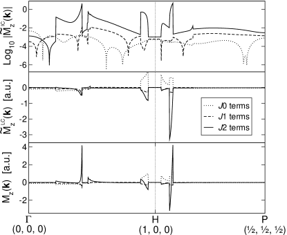
Figure 3: Decomposition of the quantity $M_{z}({\bf k})=\widetilde{M}^{\rm LC}_{z}({\bf k})+\widetilde{M}^{\rm IC}_{z}({\bf k})$ plotted in the lower panel of Fig. 2 into contributions from the three types of terms defined in Table 3.

VII Conclusions

We have presented a first-principles scheme, based on partially occupied Wannier functions, to efficiently calculate the orbital magnetization of metals using the formally correct definition for periodic crystals, Eq. (1). The localization of the WFs in real space is exploited to carry out the necessary Brillouin-zone integrals by Wannier interpolation, starting from the real-space matrix elements of a small set of operators [Eqs. (74) and (78–80)]. The same type of strategy has previously been used to evaluate other quantities, e.g., the anomalous Hall conductivity Wang06 and the electron-phonon coupling matrix elements, Giustino_07 which are notoriously difficult to converge with respect to ${\bf k}$-point sampling.

As a first application, we used the method to calculate the spontaneous orbital magnetization of the bulk ferromagnetic transition metals. Compared to the AHC in these systems, we find that the orbital magnetization, while displaying similar spiky features in ${\bf k}$-space around the Fermi surface, is somewhat less demanding. Nevertheless, well-converged results still require a fairly dense sampling of the BZ, making it advantageous to use an accurate interpolation scheme instead of a direct first-principles calculation for every integration point.

Besides being computationally very efficient, the Wannier interpolation approach has the appealing feature that the evaluation of Eq. (1) is done outside the first-principles code in a post-processing step. The algorithm is in fact completely independent of such details as the basis set used in the first-principles calculation. As a result, the calculation of the orbital magnetization only needs to be coded once in the Wannier package, and the same code can be reused by interfacing it with any desired ${\bf k}$-space electronic structure code.

We envision several possible applications for the method developed in this work. One example is the study of enhanced orbital moments in low-dimensional systems, such as magnetic nanowires deposited on metal surfaces.gambardella-nature02 ; komelj-prb02 The method is not restricted to the spontaneous orbital magnetization in ferromagnets; changes in magnetization induced by perturbations that preserve the lattice periodicity can also be treated within the same framework. One such application is the determination of the NMR shielding tensors using the so-called “converse” approach.Thonhauser_09a ; Thonhauser_09b At present the converse approach, using Eq. (1) for the induced orbital magnetization, has only been applied to molecules and bulk insulators. However, by combining it with the present Wannier-based formulation, it could provide a practical route for the evaluation of the shielding tensors in metals, a problem which is known to demand a very dense sampling of the Brillouin zone.davezac-prb07

Appendix A Derivation of Eq. (64)

With the help of Eq. (23), the left-hand-side of Eq. (64) can be written as

$${\rm tr}\left[f^{{\rm H}}\left(U^{\dagger}\mathbbm{A}_{\alpha}U\right)f^{{\rm H}}\left(U^{\dagger}\mathbbm{B}_{\beta}U\right)\right]\,.$$ (101)

Next we use the identities

$$U^{\dagger}\mathbbm{A}_{\alpha}U=\mathbbm{A}_{\alpha}^{{\rm H}}-J_{\alpha}^{{\rm H}}$$ (102)

and

$$U^{\dagger}\mathbbm{B}_{\beta}U=\mathbbm{B}_{\beta}^{{\rm H}}-\mathbbm{H}^{{\rm H}}J_{\beta}^{{\rm H}}$$ (103)

(these can be obtained by inserting Eq. (15) into the definitions (28) and (33)), to recast Eq. (101) as

$$\sum_{nm}^{J}\,f_{n}^{{\rm H}}\left(\mathbbm{A}^{{\rm H}}_{\alpha,nm}-J^{{\rm H}}_{\alpha,nm}\right)f^{{\rm H}}_{m}\left(\mathbbm{B}^{{\rm H}}_{\beta,mn}-\overline{\varepsilon}_{m}J^{{\rm H}}_{\beta,mn}\right).$$ (104)

Now we note that

$$f^{{\rm H}}_{m}\mathbbm{B}^{{\rm H}}_{\beta,mn}=if^{{\rm H}}_{m}\langle u^{{\rm H}}_{m}|\hat{H}|\partial_{\beta}u^{{\rm H}}_{n}\rangle=\overline{\varepsilon}_{m}\mathbbm{A}^{{\rm H}}_{\beta,mn}\,,$$ (105)

since by construction the occupied Hamiltonian-gauge states are eigenstates of the Hamiltonian (see Sec. II.2). Using Eq. (105) in the expression (104), factoring out $\overline{\varepsilon}_{m}$, and invoking Eq. (102) once more, yields

$${\rm tr}\left[f^{{\rm H}}\left(U^{\dagger}\mathbbm{A}_{\alpha}U\right)f^{{\rm H}}\mathbbm{H}^{{\rm H}}\left(U^{\dagger}\mathbbm{A}_{\beta}U\right)\right]\,.$$ (106)

Inserting $1=U^{\dagger}U$ between $f^{{\rm H}}$ and $\mathbbm{H}^{{\rm H}}$, the right-hand-side of Eq. (64) is finally obtained.

References

- (1) R. M. Martin, Electronic Structure, Basic Theory and Practical Methods (Cambridge University Press, Cambridge 2004).
- (2) A. J. P. Meyer and G. Asch, J. Appl. Phys. 32, S330 (1961).
- (3) G. G. Scott, Rev. Mod. Phys. 34, 102 (1962).
- (4) S. Qiao, A. Kimura, H. Adachi, K. Iori, K. Miyamoto, T. Xie, H. Namatame, M. Taniguchi, A. Tanaka, T. Muro, S. Imada, and S. Suga, Phys. Rev. B 70, 134418 (2004).
- (5) H. J. Gotsis and I. I. Mazin, Phys. Rev. B 68, 224427 (2003).
- (6) J. W. Taylor, J. A. Duffy, A. M. Bebb, M. R. Lees, L. Bouchenoire, S. D. Brown, and M. J. Cooper, Phys. Rev. B 66, 161319(R) (2002).
- (7) P. Gambardella, A. Dallmeyer, K. Maiti, M. C. Malagoli, W. Eberhardt, K. Kern, and C. Carbone, Nature 416, 301 (2002).
- (8) X. L. Qi, T. L. Hughes, and S. C. Zhang, Phys. Rev. B 78, 195424 (2008).
- (9) A. M. Essin, J. E. Moore, and D. Vanderbilt, Phys. Rev. Lett. 102, 146805 (2009).
- (10) S. Coh, D. Vanderbilt, A. Malashevich, and I. Souza, Phys. Rev. B 83, 085108 (2011), and references cited therein.
- (11) D. Ceresoli, N. Marzari, M. G. Lopez, and T. Thonhauser, Phys. Rev. B 81, 184424 (2010).
- (12) T. Thonhauser, D. Ceresoli, A. A. Mostofi, N. Marzari, R. Resta, and D. Vanderbilt, J. Chem. Phys. 131, 101101 (2009).
- (13) T. Thonhauser, D. Ceresoli, and N. Marzari, Int. J. Quantum Chem. 109, 3336 (2009).
- (14) D. Ceresoli, U. Gerstmann, A. P. Seitsonen, and F. Mauri, Phys. Rev. B 81, 060409(R) (2010).
- (15) R. Wu, First Principles Determination of Magnetic Anisotropy and Magnetostriction in Transition Metal Alloys, Lecture Notes in Phys. 580 (Springer, Berlin, 2001).
- (16) S. Sharma, S. Pittalis, S. Kurth, S. Shallcross, J. K. Dewhurst, and E. K. U. Gross, Phys. Rev. B 76, 100401(R) (2007).
- (17) T. Thonhauser, D. Ceresoli, D. Vanderbilt, and R. Resta, Phys. Rev. Lett. 95, 137205 (2005).
- (18) D. Xiao, J. Shi, and Q. Niu, Phys. Rev. Lett. 95, 137204 (2005).
- (19) D. Ceresoli, T. Thonhauser, D. Vanderbilt, and R. Resta, Phys. Rev. B 74, 024408 (2006).
- (20) J. Shi, G. Vignale, D. Xiao, and Q. Niu, Phys. Rev. Lett. 99, 197202 (2007).
- (21) T. Thonhauser, Int. J. Mod. Phys. B 25, 1429 (2011).
- (22) C. J. Pickard and M. C. Payne, Phys. Rev. B 62, 4383 (2000); M. Iannuzzi and M. Parrinello, ibid. 64, 233104 (2001).
- (23) N. Marzari and D. Vanderbilt, Phys. Rev. B 56, 12847 (1997).
- (24) I. Souza, N. Marzari, and D. Vanderbilt, Phys. Rev. B 65, 035109 (2001).
- (25) X. Wang, J. R. Yates, I. Souza, and D. Vanderbilt, Phys. Rev. B 74, 195118 (2006).
- (26) I. Souza and D. Vanderbilt, Phys. Rev. B 77, 054438 (2008).
- (27) D. Xiao, M.-C. Chang, and Q. Niu, Rev. Mod. Phys. 82, 1959 (2010).
- (28) In a metal, would also contain a -function contribution on the Fermi surface arising from the discontinuity in . This is omitted here, since it is clear from Eq. (1) that no special Fermi-surface contribution enters the final formula for .
- (29) A decomposition similar to that of Eq. (60) can be made for the Berry curvature, Eq. (III.1.1). The 0, 1, and 2 terms then correspond respectively to the “”, “-,” and “-” terms of Ref. Wang06, .
- (30) A. Dal Corso and A. MoscaConte, Phys. Rev. B 71, 115106 (2005).
- (31) J. P. Perdew, K. Burke, and M. Ernzerhof, Phys Rev. Lett. 77, 3865 (1996).
- (32) P. Giannozzi et al., J. Phys.: Condens. Matter 21, 395502 (2009), http://www.quantum-espresso.org .
- (33) A. A. Mostofi, J. R. Yates, Y.-S. Lee, I. Souza, D. Vanderbilt, and N. Marzari, Comput. Phys. Commun. 178, 685 (2008), http://www.wannier.org .
- (34) H. J. Monkhorst and J. D. Pack, Phys. Rev. B 13, 5188 (1976).
- (35) X. Wang, D. Vanderbilt, J. R. Yates, and I. Souza, Phys. Rev. B 76, 195109 (2007).
- (36) C. J. Pickard and F. Mauri, Phys. Rev. B 63, 245101 (2001).
- (37) F. Freimuth, Y. Mokrousov, D. Wortmann, S. Heinze, and S. Blügel, Phys. Rev. B 78, 035120 (2008).
- (38) A. Wensauer and U. Rössler, Phys. Rev. B 69, 155302 (2004).
- (39) S. Rohra and A. Görling, Phys. Rev. Lett. 97, 013005 (2006).
- (40) J. M. Morbec and K. Capelle, Int. J. Quant. Chem. 108, 2433 (2008).
- (41) S. H. Abedinpour, G. Vignale, and I. V. Tokatly, Phys. Rev. B 81, 125123 (2010).
- (42) Y. Yao, L. Kleinman, A. H. MacDonald, J. Sinova, T. Jungwirth, D.-S. Wang, E. Wang, and Q. Niu, Phys. Rev. Lett. 92, 037204 (2004).
- (43) The importance of the terms in is not surprising, given that the Wannier matrix elements of , which determine the full orbital magnetization in the limit of an isolated molecule, only enter through those terms.
- (44) These results were obtained from Ref. Ceresoli_10b, and its supplemental material, as well as from a personal communication with the authors of Ref. Ceresoli_10b, .
- (45) F. Giustino, M. L. Cohen, and S. G. Louie, Phys. Rev. B 76, 165108 (2007).
- (46) M. Komelj, C. Ederer, J. W. Davenport, and M. Fähnle, Phys. Rev. B 66, 140407(R) (2002).
- (47) M. d’Avezac, N. Marzari, and F. Mauri, Phys. Rev. B 76, 165122 (2007).