Low-lying Dirac operator eigenvalues, lattice effects and random matrix theory

Abstract:

Recently, random matrix theory predictions for the distribution of low-lying Dirac operator eigenvalues have been extended to include lattice effects for both staggered and Wilson fermions. We computed low-lying eigenvalues for the Hermitian Wilson-Dirac operator and for improved staggered fermions on several quenched ensembles with size $\approx 1.5$ fm. Comparisons to the expectations from RMT with lattice effects included are made. Wilson RMT describes our Wilson data nicely. For improved staggered fermions we find strong indications that taste breaking effects on the low-lying spectrum disappear in the continuum limit, as expected from staggered RMT.

1 Chiral perturbation theory including lattice artifacts

In recent years, chiral perturbation theory ($\chi$PT) has been extended to include lattice artifacts for both staggered [1] and Wilson fermions [2]. In this talk, we will be concerned only with the $\epsilon$-regime of $\chi$PT where the zero momentum modes dominate. Thus, we consider only the zero momentum part of the chiral Lagrangian

$${\cal L}=-\frac{1}{2}m\Sigma\mbox{Tr}\left(U+U^{\dagger}\right)+a^{2}{\cal V}~{}.$$ (1)

Here ${\cal V}$ describes the lattice artifacts. For staggered fermions these are dominated by taste breaking terms [1]

$${\cal V}=-\frac{1}{2}C_{4}\mbox{Tr}\left(\xi_{\mu 5}U\xi_{5\mu}U^{\dagger}+h.c.\right)+\dots~{},$$ (2)

where we displayed only the term that dominates the pseudoscalar mass splittings explicitly. Here $\xi_{\mu}=\gamma_{\mu}^{\ast}$ are taste matrices. This is also the term that dominates the lattice effects in the low-lying Dirac spectrum in the regime of weak taste breaking.

For Wilson fermions, the lattice artifact terms are [2]

$${\cal V}=W_{8}\mbox{Tr}\left(U^{2}+U^{\dagger 2}\right)+W_{6}\left[\mbox{Tr}\left(U+U^{\dagger}\right)\right]^{2}+W_{7}\left[\mbox{Tr}\left(U-U^{\dagger}\right)\right]^{2}~{}.$$ (3)

The two-trace terms, with coefficients $W_{6}$ and $W_{7}$, are suppressed at large $N_{c}$. We will neglect them here and only keep the one-trace correction term, proportional to $W_{8}$.

2 Random matrix theory including lattice artifacts

The $\epsilon$-regime of $\chi$PT  at leading order, can equivalently be described by a chiral random matrix theory (RMT). For continuum QCD, the Dirac operator is represented in RMT as

$${\cal D}_{0}=\left(\begin{array}[]{cc}0&iW\\ iW^{\dagger}&0\end{array}\right)$$ (4)

with $W$ a random $(N+\nu)\times N$ complex matrix, when working in a sector with index (topological charge) $\nu$.

2.1 Staggered RMT

For staggered fermions, the Dirac operator in staggered RMT (SRMT) is represented as [3]

$${\cal D}_{stag}={\cal D}_{0}\otimes\mathbb{I}_{4}+a{\cal T}~{},\qquad{\cal T}_{C_{4}}=\left(\begin{array}[]{cc}A_{\mu}&0\\ 0&B_{\mu}\end{array}\right)\otimes\xi_{\mu 5}~{}.$$ (5)

Here $\mathbb{I}_{4}$ is the identity matrix in taste space and ${\cal T}$ denotes the taste beaking terms. The dominant taste-breaking term, corresponding to the term explicitly shown in Eq. (2), denoted by ${\cal T}_{C_{4}}$ is shown in the second part. There, $A_{\mu}$ and $B_{\mu}$ are random Hermitian matrices of size $(N+\nu)\times(N+\nu)$ and $N\times N$, respectively. The width of the Gaussion distributions of $A_{\mu}$ and $B_{\mu}$ is proportinal to $C_{4}$. The dimensionless combination $a^{2}C_{4}V$ controls the strength of the taste breaking in SRMT.

Without the taste-breaking terms $a{\cal T}$ (i.e., in the continuum limit) the eigenvalues of the Dirac operator come in degenerate quartets. For weak taste breaking, $a^{2}C_{4}V\ll 1$, the quartets of eigenvalues are split, at leading order in a perturbation by $a{\cal T}_{C_{4}}$, into pairs of eigenvalues with splitting $\Delta\lambda_{quart}$ [3]. The pairs of eigenvalues, in turn, are split, for weak taste breaking, at second order in a perturbation by $a{\cal T}_{C_{4}}$, with subdominant splitting $\Delta\lambda_{pair}$. So SRMT predicts

$$\frac{\Delta\lambda_{quart}}{\lambda}\propto a\sqrt{C_{4}V}~{},\qquad\frac{\Delta\lambda_{pair}}{\lambda}\propto a^{2}C_{4}V~{}.$$ (6)

2.2 Wilson RMT

For Wilson fermions, the Dirac operator in Wilson RMT (WRMT) is represented as [4]

$${\cal D}_{W}={\cal D}_{0}+\tilde{a}\left(\begin{array}[]{cc}A&0\\ 0&B\end{array}\right)~{},$$ (7)

with $A$ and $B$ random Hermitian matrices of size $(N+\nu)\times(N+\nu)$ and $N\times N$, respectively, that represent the chiral symmetry breaking Wilson term of the lattice Wilson-Dirac operator.

Akemann et al., Ref. [4], have worked out the eigenvalue distribution of the Hermitian Wilson-Dirac operator, $H_{W}=\gamma_{5}\left(D_{W}+m_{0}\right)$, or its RMT equivalent, ${\cal H}_{W}=\gamma_{5}\left({\cal D}_{W}+\tilde{m}\right)$ with

$$\hat{m}=m\Sigma V=2\tilde{m}N\quad\text{and}\quad\hat{a}^{2}=a^{2}W_{8}V=\frac{1}{2}\tilde{a}^{2}N$$ (8)

held fixed, using Wilson $\chi$PT. The results were reproduced directly from WRMT in [5]. In Eq. (8) $m$ is a suitably subtracted version of the bare mass $m_{0}$. In the analytical predictions, the eigenvalues are rescaled with $\Sigma V$ in the lattice QCD case, and with $2N$ for WRMT.

3 Results for staggered fermions compared to SRMT

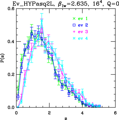
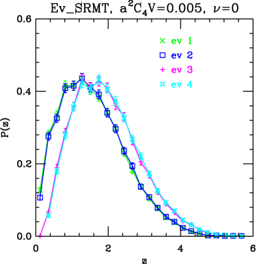
Figure 1: Distributions of the lowest four (rescaled) eigenvalues for $Q=0$. The left panel shows the staggered Dirac eigenvalues from an ensemble of $a=0.093$ fm and $L=1.5$ fm configurations, the right panel the eigenvalues from a MC generated SRMT ensemble with taste-breaking parameter $a^{2}C_{4}V=0.005$.

We have computed low lying staggered eigenvalues for various staggered actions with different smearings using ensembles of pure gauge configurations generated with the Iwasaki gauge action. As observed previously [6], the quartet structure, and the appearance of clearly distinct would-be zeromodes, becomes more visible with increased smearing and with smaller lattice spacing. Here we show and discuss some results with our best staggered action, a HISQ-like action but with first a HYP(ii) smearing step [7] instead of a fat7 smearing step and subsequent unitarization, followed by an asq step with the appropriate Lepage term, denoted by “HYPasq2L”. For more details and further results we refer to Ref. [8]. Here we illustrate a few of our findings.

We compare distributions of the lowest four eigenvalues from $\sim 1200$ $Q=0$ configurations at $a=0.093$ fm and $L=1.5$ fm with Monte Carlo generated SRMT $\nu=0$ eigenvalue distributions for the taste violating parameter $a^{2}C_{4}V=0.005$ in Fig. 1. The LQCD eigenvalues are rescaled by $\Sigma V$ and the SRMT ones by $2N$ for the comparison. The distributions agree quite nicely.

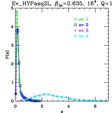
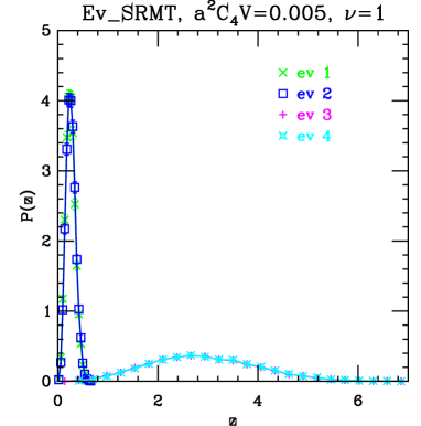
Figure 2: Same as Fig. 1 but for $|Q|=1$ ($\nu=1$) configurations. Here, the lowest two eigenvalues are the would-be zeromodes.

Fig. 2 shows the distribution of the lowest four eigenvalues, including the two positive would-be zeromodes, for $\sim 2000$ $|Q|=1$ configurations of the same gauge ensemble and $\nu=1$ SRMT MC generated eigenvalue distributions. Again, the distributions agree quite nicely, although the distributions of the would-be zeromodes for the staggered Dirac operator have somewhat longer tails than their SRMT counterparts. In the SRMT distributions, the peak height of the “would-be zeromodes” turns out to be the feature most sensitive to the value of the taste-breaking parameter $a^{2}C_{4}V$. It is from this peak height that we estimated that $a^{2}C_{4}V=0.005$ provides the best match to the LQCD data.

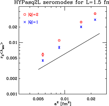
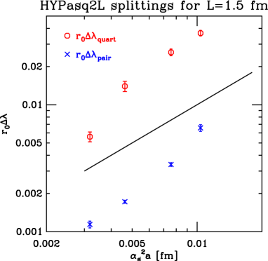
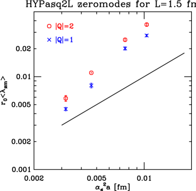
Figure 3: The vanishing of the splitting (left panels) and would-be zeromodes (right panels) – shown is the average over the would-be zeromodes with slightly positive eigenvalues – as a function of $a^{2}$ (top) or $\alpha_{s}^{2}a$ (bottom). The inclined straight lines show the behavior to be tested in the plots.

According to the SRMT prediction, Eq. (6), the dominant splitting $\Delta\lambda_{quart}$ should vanish, at fixed volume, like $\alpha_{s}^{n}a$, where $n$ depends on the degree of improvement, while the subdominat splitting $\Delta\lambda_{pair}$ should vanish like $a^{2}$. We compare these predictions, as well as the vanishing of the would-be zeromodes, for fixed lattice size $L=1.5$ fm, in Fig. 3. The would-be zeromodes appear to vanish a little faster than $a^{2}$. The behavior of the splittings is less clear, with a vanishing as $a^{2}$ favored for the smaller splitting, $\Delta\lambda_{pair}$. But both splittings certainly vanish in the continuum limit, as expected.

4 Results for Wilson fermions compared to WRMT

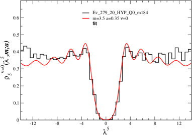
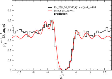
Figure 4: The eigenvalues density of $H_{w}$ with bare mass $am_{0}=-0.184$ on an ensemble of $a=0.075$ fm and $L=1.5$ fm configurations with $Q=0$ (left) and $|Q|=1$ (right). The $Q=0$ distribution was used to obtain the WRMT parameters. The same parameters are used for the $|Q|=1$ WRMT distribution on the right.

We computed the low-lying eigenvalues of the Hermitian Wilson-Dirac operator $H_{W}$ on the $Q=0$ and $|Q|=1$ configurations of an ensemble with lattice spacing $a=0.075$ fm and size $L=1.5$ fm, as before generated with the Iwasaki gauge action, for two bare quark masses. To suppress dislocations we smoothened the gauge field with one HYP smearing step before constructing the Wilson-Dirac operator.

RMT predictions are made for sectors with a given index $\nu$. Such an index can be defined from the real eigenvalues of the Wilson-Dirac operator and the chiralities of the corresponding eigenmodes Ref. [4]. Equivalently, the index can be obtained from the spectral flow of the Hermitian Wilson-Dirac operator [9]. In both cases the definition depends on a cut: the maximum real eigenvalue kept or the mass at which the flow is terminated. For our setup we found little dependence on this cut and good agreement with the cheaper definition of topological charge with six HYP smearings and use of an improved $F{}^{*}F$ operator [10].

To compare the sepctrum of the Hermitian Wilson-Dirac operator with predictions from WRMT, we used the distribution in the $Q=0$ sector with the bare mass corresponding to a lighter quark mass to find the WRMT parameters $\hat{m}$ and $\hat{a}$, and the eigenvalue rescaling factor $\Sigma V$ that best describe our data, see Fig. 4 (left). Using the same parameter values, WRMT then predicts the $|Q|=1$ distribution that can be compared with the measured one, see Fig. 4 (right). We find a nice agreement with the measured (histogrammed) distribution.

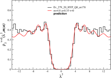
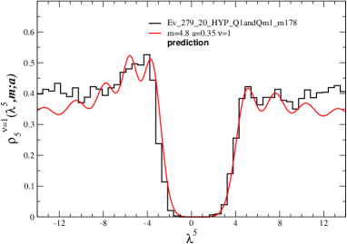
Figure 5: Same as Fig. 4 but for bare mass $am_{0}=-0.178$. The same WRMT parameters, up to changing $\hat{m}$ according to the bare mass difference, $\delta\hat{m}=\delta m_{0}\Sigma V$, were used.

Changing only the bare quark mass in $H_{W}$ should leave the WRMT parameter $\hat{a}$, and the rescaling factor $\Sigma V$ unchanged, while the WRMT parameter $\hat{m}$ should be changed by $\delta\hat{m}=\delta m_{0}\Sigma V$, Eq. (8), where $\delta m_{0}$ is the difference in bare quark mass. We, therefore, have parameter free predicitions for the eigenvalue distributions with the second quark mass. As shown in Fig. 5, these predictions work well.

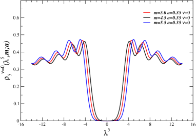
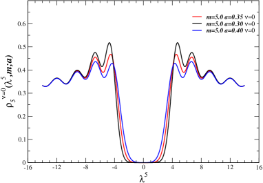
Figure 6: The dependence of the distribuion of the eigenvalue density of $\cal{H}_{W}$ on $\hat{m}$ (left) and on $\hat{a}$ (right).

We illustrate the sensitivity of the analytic WRMT distributions to the WRMT parameters $\hat{m}$ in Fig. 6 (left) and to $\hat{a}$ in Fig. 6 (right). For the ensemble considered in Figs. 4 and 5 we can obtain $\hat{m}$ to an accuracy of about $0.5$ and $\hat{a}$ to about $0.05$. Going to smaller lattice spacing will increase the accuracy. For further details and more tests, see [11]. A. Deuzeman presented results from a similar study at this conference with compatible results [12].

References

-
[1]
W.-J. Lee and S.R. Sharpe,
Phys. Rev. D 60 (1999) 114503 [arXiv:heplat/9905023];
C. Aubin and C. Bernard, Phys. Rev. D 68 (2003) 034014 [arXiv:heplat/0304014]. -
[2]
S.R. Sharpe and R.L. Singleton,
Phys. Rev. D 58 (1998) 074501 [arXiv:heplat/9804028];
O. Bär, G. Rupal and N. Shoresh. Phys. Rev. D 70 (2004) 034508 [arXiv:heplat/0306021]. - [3] J.C. Osborn, Phys. Rev. D 83 (2011) 034505 [arXiv:1012.4837].
- [4] G. Akemann, P.H. Damgaard, K. Splittorff and J.J.M. Verbaarschot, Phys. Rev. D 83 (2011) 085014 [arXiv:1012.0752].
- [5] G. Akemann and T. Nagao, arXiv:1108.3035.
-
[6]
E. Follana, A. Hart and C.T.H. Davies,
Phys. Rev. Lett. 93 (2004) 241601 [arXiv:hep-lat/0406010];
E. Follana, A. Hart, C.T.H. Davies and Q. Mason, Phys. Rev. D 72 (2005) 054501 [arXiv:hep-lat/0507011]. - [7] W. Lee and S.R. Sharpe, Phys. Rev. D 66 (2002) 114501 [arXiv:hep-lat/0208018].
- [8] Urs M. Heller, in preparation.
- [9] R.G. Edwards, U.M. Heller and R. Narayanan, Nucl. Phys. B 535 (1998) 403 [arXiv:hep-lat/9802016].
- [10] T.A. DeGrand, A. Hasenfratz, and T.G. Kovacs, Nucl. Phys. B 505 (1997) 417 [arXiv:heplat/9705009].
- [11] P.H. Damgaard, U.M. Heller and K. Splittorff, arXiv:1110.2851.
- [12] A. Deuzeman, U. Wenger and J. Wuilloud, these proceedings, and arXiv:1110.4002.