Finite-size scaling considerations on the ground state microcanonical temperature in entropic sampling simulations

Abstract

In this work we discuss the behavior of the microcanonical temperature $\frac{\partial S(E)}{\partial E}$ obtained by means of numerical entropic sampling studies. It is observed that in almost all cases the slope of the logarithm of the density of states $S(E)$ is not infinite in the ground state, since as expected it should be directly related to the inverse temperature $\frac{1}{T}$. Here we show that these finite slopes are in fact due to finite-size effects and we propose an analytic expression $a\ln(bL)$ for the behavior of $\frac{\varDelta S}{\varDelta E}$ when $L\rightarrow\infty$. To test this idea we use three distinct two-dimensional square lattice models presenting second-order phase transitions. We calculated by exact means the parameters $a$ and $b$ for the two-states Ising model and for the $q=3$ and $4$ states Potts model and compared with the results obtained by entropic sampling simulations. We found an excellent agreement between exact and numerical values. We argue that this new set of parameters $a$ and $b$ represents an interesting novel issue of investigation in entropic sampling studies for different models.

1 Introduction

Monte Carlo (MC) entropic sampling simulationsLee93 ; Oliveira96 ; Oliveira98 ; Wang00 have attracted a great deal of attention in the last years due to its capability to calculate directly the entropy $S(E)=k_{B}\ln\Omega(E)$ of a variety of systems. This definition of entropy in terms of the number of microstates $\Omega(E)$ with energy $E$ has been the cornerstone of statistical mechanics since its introduction by BoltzmannCallen85 . Hence the computation of such quantity by numerical means is of great importance to accurately locate and characterize phase transitions. The motivation for the development of these new MC methods resides in the fact that conventional methods exhibit long time scale problems. These methods are based on the estimation of all possible states (or configurations) for an energy level $E$ of the system which is being studied. Since the partition function for a given model in statistical physics can be expressed in terms of the density of states $\Omega(E)$, if one can estimate this quantity with high accuracy it is possible to construct the partition function as $Z=\sum_{E}\Omega(E)e^{-E/k_{B}T}$, essentially solving the model. Here $k_{B}$ denotes the Boltzmann constant. Therefore, one can study the full temperature range without further simulation runs. The most celebrated approach in this direction is the Wang-Landau (WL) sampling WangLandau01a ; WangLandau01b . This method measures an a priori unknown density of states of a given system iteratively by performing a random walk in energy space and sampling configurations with probability proportional to the reciprocal of the density of states, resulting in a “flat” histogram.

Conversely, analyzing the results of any entropic sampling simulation, the logarithm of the density of states corresponds exactly to the definition of entropy. The Boltzmann constant $k_{B}$ ensures the agreement with the Kelvin scale of temperature, defined by

$$\frac{1}{T}=\frac{\partial S(E)}{\partial E}.$$ (1)

One should therefore expect a divergence of $\frac{\partial S(E)}{\partial E}$ at the ground state temperature. Nevertheless what we see in most plots of the logarithm of the density of states obtained by entropic sampling simulations is a clear finite slope in the ground state. The reason for this apparent contradiction are the finite-size effects. In fact for finite systems, from small to large, the thermodynamics is a rather controversial issueHill62 . In downscale one have problems defining phase transitionsGulminelli99 ; Borrmann00 , the equivalence between ensemblesGulminelli03 ; Fiore13 , the extensivity of thermodynamical variablesGross05 and so on. Accordingly, in this work we intend to shed some light on the reason why the slope of the logarithm of the density of states, obtained by entropic sampling procedures, is not infinite in the ground state, where the inverse temperature diverges. Our proposal may provide a supplementary way of investigation for any entropic MC simulation.

The outline of this paper is as follows: In section II we present a finite-size scaling analysis of the microcanonical temperature. In section III we define the simulation procedure. In section IV the simulation results are discussed. Section V is devoted to the summary and concluding remarks.

2 Finite-Size Scaling Behavior of the Microcanonical Temperature

In Fig. 1 we show the logarithm of the density of states of the 2D Ising model on a square lattice with nearest neighbors interactions obtained by Wang-Landau sampling for two lattice sizes: $L=32,64$. One can see that indeed the slopes are not infinite at the ground state. Moreover, this behavior is also observed in the exact results obtained by Beale Beale96 . This situation resembles that of the magnetization in the Ising model, which for an infinite system drops to zero exactly at the critical temperature but presents a tail for finite-size lattices.

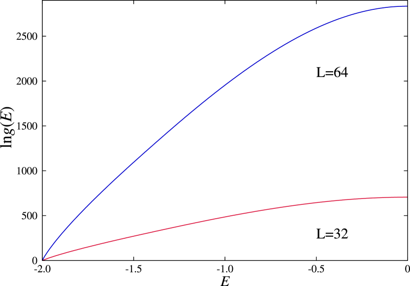
Figure 1: (Color online) Logarithm of the density of states obtained by Wang-Landau sampling for the 2D Ising model for $L=32,64$ as functions of the energy per spin.

For any finite-size lattice of a model with a discrete energy landscape, the smallest $\varDelta E$ from the ground state is constant for all lattice sizes:

$$\varDelta E=const.$$ (2)

Therefore, the limit in the derivative

$$\frac{\partial S}{\partial E}=\lim_{\varDelta E\to 0}\frac{\varDelta S}{\varDelta E}$$ (3)

becomes exact only if $L\rightarrow\infty$ ($E_{min}\rightarrow-\infty$), where $L$ is the linear lattice size. As a result, what we have to do is to investigate how $\frac{\varDelta S}{\varDelta E}$ diverges as $L\rightarrow\infty$. Let us consider three two-dimensional systems: the Ising model, the $q=3$ Potts model and the $q=4$ Potts model on square lattices and with nearest neighbors interactions.

The 2D Ising model for a ferromagnet on a square lattice is described by the Hamiltonian barkema

$${\cal H}=-J\sum_{\langle i,j\rangle}\sigma_{i}\sigma_{j},$$ (4)

where $\sigma_{i}=\pm 1$ represents a spin at lattice site $i$ and the notation $\langle i,j\rangle$ indicates that the sites $i$ and $j$ appearing in the sum are nearest neighbors on the lattice with interaction constant $J>0$. In the ground state all the spins are aligned in the same direction, $\sigma_{i}=+1$, for instance. If a single spin is flipped, it looses four negative links and gains four positive ones. The energy gap between the ground state and the next state is therefore $\varDelta E=4-(-4)=8$, where we take the coupling constant $J$ as 1.

By its turn, the Potts model, proposed by Potts in the early 1950’s is an extension of the two states Ising model to $q>2$ states. In this model, to each lattice site is attached a spin variable $\sigma_{i}$ (defined on each site $i$) which takes on integer values $1,\ldots,q$. Adjacent sites have an attractive interaction energy $-J$ whenever they are equal or $0$ otherwise. The Hamiltonian of the $q$-states ferromagnetic model ($J>0$) on a square lattice can be written as barkema

$${\cal H}=-J\sum_{\langle i,j\rangle}\delta_{\sigma_{i}\sigma_{j}},$$ (5)

where $\delta$ is the Kronecker $\delta-$symbol, and the sum runs over all nearest neighbors of $\sigma_{i}$. The ground state has $q$ distinct configurations with all spins in the state $1,2,...$ or $q$. If a single spin is changed it looses four negative links and does not gain any link, since all the neighbors will have a different label. In this case the difference between the state of minimum energy and the next one is $\varDelta E=0-(-4)=4$, where again we set $J=1$.

In the Ising model the ground state has two configurations and the next higher level $2L^{2}$, yielding $\varDelta S=\ln 2+2\ln L-\ln 2$ and $\varDelta E=8$, giving

$$\frac{\varDelta S}{\varDelta E}=\frac{\ln L}{4}=0.25\ln L.$$ (6)

For notational simplicity we set $k_{B}=1$.

The $q=3$ Potts model has three configurations in the ground state and $6L^{2}$ in the first higher level. In this case we have $\varDelta S=\ln 6+2\ln L-\ln 3=\ln 2+2\ln L$ and $\varDelta E=4$, such that

$$\frac{\varDelta S}{\varDelta E}=\frac{\ln 2}{4}+\frac{\ln L}{2}=0.5\ln(2^{1/2}L)$$ (7)

Finally for the $q=4$ Potts model we have four configurations in the ground state and $12L^{2}$ in the second level and here $\varDelta S=\ln 12+2\ln L-\ln 4=\ln 3+2\ln L$ and $\varDelta E=4$, resulting in

$$\frac{\varDelta S}{\varDelta E}=\frac{\ln 3}{4}+\frac{\ln L}{2}=0.5\ln(3^{1/2}L)$$ (8)

In all examples above we see that $\frac{\varDelta S}{\varDelta E}$ has a logarithmic dependence on $L$ given by

$$\frac{\varDelta S}{\varDelta E}=a\ln(bL).$$ (9)

Each model has a couple of parameters $a$ and $b$, which governs the way $\frac{\varDelta S}{\varDelta E}$ diverges when $L\rightarrow\infty$. For these models we have therefore calculated the exact values to $a$ and $b$, which we display in Table 1.

	Model	$a$	$b$
	Ising	$0.25$	$1$
	$q=3$ Potts	$0.5$	$\sqrt{2}$
	$q=4$ Potts	$0.5$	$\sqrt{3}$

Table 1: Exact values of the parameters $a$ and $b$ for the Ising model, the $q=3$ Potts model and the $q=4$ Potts model.

3 Entropic Sampling Simulations

The conventional Wang-Landau method WangLandau01a ; WangLandau01b is based on the fact that if one performs a random walk in energy space with a probability proportional to the reciprocal of the density of states, a flat histogram is generated for the energy distribution. Since the density of states produces huge numbers, instead of estimating $\Omega(E)$, the simulation is performed for $S(E)\equiv\ln\Omega(E)$. At the beginning, we set $S(E)=0$ for all energy levels. The random walk in the energy space runs through all energy levels from $E_{min}$ to $E_{max}$ with a probability $p(E\rightarrow E^{\prime})=\min(\exp{[S(E)-S(E^{\prime})]},1)$, where $E$ and $E^{\prime}$ are the energies of the current and the new possible configurations, respectively. In fact we begin with any configuration (a ground state configuration, for example), and a new possible configuration is obtained by changing a single spin state. If the current density of states of this energy level $E^{\prime}$ is less than or equal to that of the present energy level $E$, then the configuration is accepted, otherwise we take a random number $r$, such that $0<r<1$ and accept this new configuration if $r<\Omega(E)/\Omega(E^{\prime})$ (or $\ln\Omega(E)-\ln\Omega(E^{\prime})>\ln r$, since we are simulating $\ln\Omega(E)$). Then, for this new accepted level or for the previous one, we update the histogram $H(E)\rightarrow H(E)+1$ and $S(E)\rightarrow S(E)+F_{i}$, where $F_{i}=\ln f_{i}$, with $f_{0}\equiv e=2.71828...$ and $f_{i+1}=\sqrt{f_{i}}$ ($f_{i}$ is the so-called modification factor). The flatness of the histogram is checked after a certain number of Monte Carlo steps (MCS) and usually the histogram is considered flat if $H(E)>0.8\langle H\rangle$, for all energies, where $\langle H\rangle$ is an average over energies. If the flatness condition is fulfilled, we update the modification factor to a finer one and reset the histogram $H(E)=0$. The entropic algorithm described above may be formally obtained from the Metropolis algorithm if one replaces the Boltzmann’s factor $e^{-E/k_{B}T}$ by the reciprocal of the density of states $1/\Omega(E)$. A histogram constructed during the Metropolis simulations is given by $H(E)=\Omega(E)e^{-E/k_{B}T}$ and is similar to a Gaussian distribution. If the Boltzmann’s factor would be replaced by the reciprocal of the density of states, the resulting histogram would be a constant. This is the reason why the flatness criterion is used during the Wang-Landau simulations to update the modification factor. Ideally, all the energy levels should be equally visited during the simulations.

Recent works Caparica12 ; Caparica14 ; Ferreira12a ; Ferreira12b have demonstrated that (a) instead of updating the density of states after every move, one ought to update it after each Monte Carlo sweep MCS (this providence avoids taking into account highly correlated configurations when constructing the density of states); (b) WL sampling should be carried out only up to $\ln f=\ln f_{final}$ defined by the canonical averages during the simulations (this saves CPU time, discarding unnecessary long simulations); and (c) the microcanonical averages should not be accumulated before $\ln f\leq lnf_{micro}$ defined by a previous study of the microcanonical averaging during the simulation (the ruled out WL levels in these averages correspond to a microcanonical termalization, since the initial configurations do not match those of maximum entropy). The adoption of these easily implementable changes leads to more accurate results and saves computational time. They investigated the behavior of the maxima of the specific heat

$$C(T)=\frac{\langle(E-\langle E\rangle)^{2}\rangle}{T^{2}}$$ (10)

and the susceptibility

$$\chi(T)=L^{2}\frac{\langle(m-\langle m\rangle)^{2}\rangle}{T},$$ (11)

where $E$ is the energy of the configurations and $m$ is the corresponding magnetization per spin, during the WL sampling for the Ising model on a square lattice. They observed that a considerable part of the conventional Wang-Landau simulation is not very useful because the error saturates. They demonstrated in detail that in general no single simulation run converges to the true value, but to a particular value of a Gaussian distribution of results around the correct value. The saturation of the error coincides with the convergence to this value. Continuing the simulations beyond this limit leads to irrelevant variations in the canonical averages of all thermodynamic variables. A later work Caparica14 proposes a criterion for halting the simulations. Applying WL sampling to a given model, beginning from $f_{5}$, we calculate the temperature of the peak of the specific heat defined in Eq. (10) using the current $\Omega(E)$ and from this time forth this mean value is updated whenever the histogram is checked for flatness. When the histogram is considered flat, we save the value of the temperature of the peak of the specific heat $T_{c}(0)$. We then update the modification factor $f_{i+1}=\sqrt{f_{i}}$ and reset the histogram $H(E)=0$. During the simulations with this new modification factor we continue calculating the temperature of the peak of the specific heat $T_{c}(t)$ whenever we check the histogram for flatness and we also calculate the following checking parameter

$$\varepsilon=|T_{c}(t)-T_{c}(0)|.$$ (12)

Ising model			$q=3$ Potts model			$q=4$ Potts model
$a$	$b$		$a$	$b$		$a$	$b$
0.24949(39)	1.0063(58)		0.49968(84)	1.4202(95)		0.50068(77)	1.721(11)
0.25036(47)	0.9953(69)		0.50059(65)	1.4061(73)		0.49965(83)	1.736(12)
0.25028(24)	0.9963(36)		0.49978(66)	1.4159(74)		0.49868(71)	1.754(10)
0.24961(29)	1.0054(43)		0.50055(76)	1.4077(84)		0.4996(11)	1.739(16)
0.25021(44)	0.9975(63)		0.50116(85)	1.4034(95)		0.5007(11)	1.722(15)
0.24972(26)	1.0056(38)		0.50142(68)	1.3993(75)		0.50008(67)	1.729(10)
0.25028(43)	0.9957(60)		0.49994(85)	1.4161(94)		0.50012(84)	1.730(12)
0.24991(31)	1.0026(46)		0.49869(85)	1.4291(97)		0.49853(73)	1.755(11)
0.25038(38)	0.9957(55)		0.50006(62)	1.4129(69)		0.49967(94)	1.736(13)
0.24956(46)	1.0054(66)		0.50089(73)	1.4057(81)		0.50153(75)	1.711(10)
0.24998(11)	1.0006(15)		0.50028(26)	1.4116(28)		0.49992(29)	1.733(44)

Table 2: Estimates by entropic sampling simulations of the parameters $a$ and $b$ for the Ising model, the $q=3$ Potts model and the $q=4$ Potts model.

If the number of MCS before verifying the histogram for flatness is chosen not too large, say $10,000$, then during the simulations with the same modification factor the checking parameter $\varepsilon$ is calculated many times. If $\varepsilon$ remains less than $10^{-4}$ until the histogram meets the flatness criterion for this WL level, then we save the density of states and the microcanonical averages and stop the simulations. When one adopts this criterion for halting the simulations, different runs stop at different final modification factors. It was also observed in Ref. Caparica14 that two independent similar finite-size scaling procedures can lead to very different results for the critical temperature and exponents, which often do not agree within the error bars. The way to overcome this difficulty is to carry out 10 independent sets of finite-size scaling simulations. In the present work, for each of theses sets and for each model (Ising, $q=3$ and $q=4$ Potts models), we performed simulations for $L=8,12,16,20,24,28,32,36,40,44,48,52,56,64,72$, and $80$ with $n=32,32,28,28,28,24,24,24,20,20,20,16,16,16,\\ 12$, and $12$ independent runs for each size, respectively.

4 Simulational Results

In fact, we used the outcomes of the simulations described in Ref. Caparica14 with $\varepsilon<10^{-4}$ for the Ising model and Ref. Caparica15 for the $q=3$ and $q=4$ Potts models. The final resulting values for $\frac{\varDelta S}{\varDelta E}$ in each case were obtained as an average over all sets. In Table 2 we display the values obtained in our entropic simulations for $a$ and $b$ for each of the considered models. The ten initial lines correspond to results obtained in each set and the last line is an average over all sets. In carrying out theses averages we tried two alternative ways: an average with unequal uncertainties Wong97 and a direct average neglecting the error bars. We observed that the second procedure leads to better results with more reliable error bars and these are the results we display in the last line of the Table 2. One can see that our results for $a$ and $b$ agree within error bars equal to $\pm 1\sigma$ with the exact results shown in Table 1 in all cases, reaching the very limit only for the parameter $a$ of the $q=3$ Potts model.

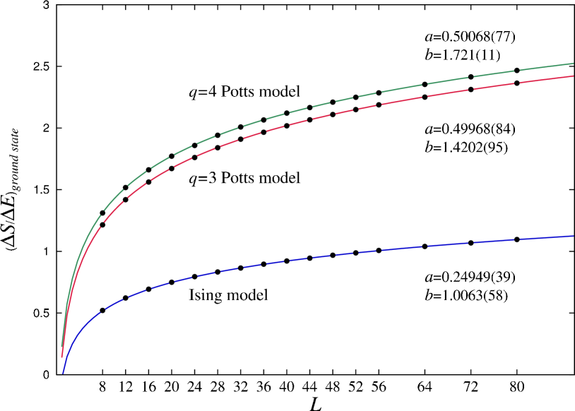
Figure 2: (Color online) Size dependence of $\frac{\varDelta S}{\varDelta E}$ at the ground state of the first set of simulations. The lines are best fitting curves of these data to $a\ln(bL)$. The error bars are smaller than the symbols.

In Fig. 2 we show the dependence of $\frac{\varDelta S}{\varDelta E}$ at the ground state on the lattice sizes using the outcomes of the first set of simulations, along with the best fitting curves to $a\ln(bL)$. The agreement is excellent.

It is noteworthy that this couple of parameters $a$ and $b$ represents a new interesting issue of investigation in studies using entropic sampling. A possible challenge would be to estimate them in the case of polymers due to the difficulty of achieving good statistics near the ground state. Furthermore it is an open question if all systems have the logarithmic behavior or eventually it could arise, for example, a power law with a coefficient and an exponent: $KL^{\kappa}$.

5 Conclusions

To summarize, in this work we analyzed the behavior of the ground state microcanonical temperature in entropic sampling simulations of spin lattice models. We verified that the expected divergence not observed in most studies are indeed related to finite-size effects. We verified that $\frac{\varDelta S}{\varDelta E}$ in the ground state diverges logarithmically and we proposed an analytic expression $a\ln(bL)$ to fit this behavior. Our exact and numerical results exhibit an excellent agreement. We have also shown that it is straightforward to calculate the constant parameters $a$ and $b$ related to the logarithmic behavior of the entropy at the ground state for the considered models. A further analysis would be to verify if this analytic expression still holds for systems with continuous energy spectrum.

- (1) J. Lee, Phys. Rev. Lett. 71, 211 (1993)
- (2) P.M.C. Oliveira, T.J.P. Penna, H.J. Herrmann, Braz. J. Phys. 26, 677 (1996)
- (3) P.M.C. Oliveira, T.J.P. Penna, H.J. Herrmann, Eur. Phys. J. B 1, 205 (1998)
- (4) J.S. Wang, L.W. Lee, Comp. Phys. Comm. 127, 131 (2000)
- (5) H.B. Callen, Thermodynamics and an Introduction to Thermostatistics (John Wiley & Sons, USA, 1985)
- (6) F. Wang, D.P. Landau, Phys. Rev. Lett. 86, 2050 (2001)
- (7) F. Wang, D.P. Landau, Phys. Rev. E 64, 056101 (2001)
- (8) T.L. Hill, J. Chem. Phys. 36, 3182 (1962)
- (9) F. Gulminelli, P. Chomaz, Phys. Rev. Lett. 84, 1402 (1999)
- (10) P. Borrmann, O. Mülken, J. Harting, Phys. Rev. Lett. 84, 3511 (2000)
- (11) P. Chomaz, F. Gulminelli, Physica A 330, 451–458 (2003)
- (12) C.E. Fiore, C.J. DaSilva, Comp. Phys. Comm. 184, 1426 (2013)
- (13) D.H.E. Gross, J.F. Kenney, J. Chem. Phys. 122, 224111 (2005)
- (14) P.D. Beale, Phys. Rev. Lett 76, 78 (1996)
- (15) M.E.J. Newman and G.T. Barkema, Monte Carlo Methods in Statistical Physics, Claredon Press, Oxford, p. 16 (Ising model), p. 120 (Potts model) (2001).
- (16) A.A. Caparica, A.G. Cunha-Netto, Phys. Rev. E 85, 046702 (2012)
- (17) A.A. Caparica, Phys. Rev. E 89, 043301 (2014)
- (18) L.S. Ferreira, A.A. Caparica, Int. J. Mod. Phys. C 23, 1240012 (2012)
- (19) L.S. Ferreira, A.A. Caparica, M.A. Neto, M.D. Galiceanu, J. Stat. Mech. 2012, P10028 (2012)
- (20) A Monte Carlo sweep consists of spin-flip trials in the 2D Ising model or monomer moves in the homopolymer.
- (21) A.A. Caparica, C.J. DaSilva, Physica A 438 (2015) pp. 447-453
- (22) S.S.M. Wong, Computational Methods in Physics and Engineering (World Scientific Publishing Co. Pte. Ltd., 1997)