DO-TH 11/30

Leptogenesis in flavor models
with type I and II seesaws

D. Aristizabal Sierra^a,, F. Bazzocchi^b,, I. de Medeiros Varzielas^c,

^aIFPA, Dep. AGO, Universite de Liege, Bat B5,
Sart Tilman B-4000 Liege 1, Belgium.

^bSISSA and INFN, Sezione di Trieste,
Via Bonomea 265, 34136 Trieste, Italy.

^cFacultät für Physik, Technische Universität Dortmund
D-44221 Dortmund, Germany.

In type I seesaw models with flavor symmetries accounting for the lepton mixing angles the CP asymmetry in right-handed neutrino decays vanishes in the limit in which the mixing pattern is exact. We study the implications that additional degrees of freedom from type II seesaw may have for leptogenesis in such a limit. We classify in a model independent way the possible realizations of type I and II seesaw schemes, differentiating between classes in which leptogenesis is viable or not. We point out that even with the interplay of type I and II seesaws there are generic classes of minimal models in which the CP asymmetry vanishes. Finally we analyze the generation of the lepton asymmetry by solving the corresponding kinetic equations in the general case of a mild hierarchy between the light right-handed neutrino and the scalar triplet masses. We identify the possible scenarios in which leptogenesis can take place.

1 Introduction

Leptogenesis is a scenario in which the baryon asymmetry of the Universe is generated first in the lepton sector and partially reprocessed into a baryon asymmetry via standard model electroweak sphaleron processes. Models for Majorana neutrino masses usually involve new interactions that satisfy the necessary conditions for leptogenesis namely lepton number violation, CP violation in the lepton sector and departure from thermodynamic equilibrium (provided by the expansion of the Universe). Type-I seesaw [1] is certainly the most well studied framework for leptogenesis, however further analysis in other Majorana neutrino mass models such as type II [2] and type III [3] seesaws has also been carried out (see ref. [4] for more details).

Even in the light of the most recent neutrino data [5, 6] there is still a strong motivation to believe the mixings in the lepton sector are governed by an underlying flavor symmetry (for a review see e.g. [7] and references therein). Indeed it is in part due to this observation that leptogenesis in Majorana neutrino mass models has been recently considered. In particular, there is an extensive literature in the case of type I seesaw [8, 9, 10, 11, 12] in which it has been shown that as long as the flavor symmetry enforces a concrete flavor mixing scheme (e.g. tribimaximal (TB) mixing) the CP violating asymmetry $\epsilon_{N}$ vanishes in the limit in which such a pattern is exact.

Viable leptogenesis requires either departures from the exact mixing scheme, or the presence of extra degrees of freedom beyond those present in the standard type I seesaw (three electroweak singlet right-handed (RH) neutrinos). Departures could arise for example via next-to-leading order corrections (${\cal O}(v_{F}^{2}/\Lambda^{2})$ corrections) where $v_{F}$ is the characteristic scale at which the flavor symmetry is broken and $\Lambda$ is a cutoff scale, or as recently proposed in [16] through renormalisation group corrections.

In ref. [11] it has been pointed out that interplay between type I and type II seesaws may allow leptogenesis at leading order (${\cal O}(v_{F}/\Lambda)$). It is the purpose of this paper to study under which conditions such scenarios are actually obtained from the inclusion of extra degrees of freedom arising from type II seesaw (involving one or more electroweak triplet scalars).

The interplay between type I and II seesaws for neutrino masses is an almost unavoidable feature of left-right symmetric models. It has been thoroughly considered in ref. [17] without assuming any underlying flavor symmetry. As a framework for leptogenesis it has been analysed in references [18, 19, 20, 21, 22], showing that the differences with the standard leptogenesis scenario can be striking. This interplay has also been considered in flavor models (see e.g. [23]). We extend upon these analyses by exploring the feasibility of leptogenesis in “hybrid” type I + type II flavor models aiming to differentiate between those that might allow leptogenesis to proceed and those in which even with the presence of the new degrees of freedom the viability of leptogenesis relies on the departures from the exact mixing scheme (as is the case when only type I seesaw is present).

The rest of the paper is organized as follows: in section 2 we set up our notation and work out the implications a flavor symmetry has in mixed I+II schemes by classifying the different possible realizations. In section 3 we elaborate on the implications for leptogenesis in the different realizations found in section 2 whereas in section 3.2 we work out the calculation of the lepton asymmetry in scenarios in which the hierarchy between the lightest RH neutrino and the electroweak triplet is mild. We present our conclusions and final remarks in section 4. In appendix A we summarize the formulas used in the calculation of the lepton asymmetry.

2 Exact mixing schemes

The presence of electroweak singlet RH neutrinos and a scalar $SU(2)$ triplet is described by the following Lagrangian

$${\cal L}={\cal L}^{I}+{\cal L}^{II}\,,$$ (1)

separating the type I and type II seesaw Lagrangians that, in the basis in which the RH neutrinos Majorana mass matrix is diagonal, can be written as

$${\cal L}^{I}= -\lambda_{ij}\overline{N}_{R_{i}}\ell_{L_{j}}\tilde{H}^{\dagger}-\frac{1}{2}\overline{N}_{R_{i}}CM_{R_{i}}\overline{N}_{R_{i}}^{T}+\mbox{h.c.}\,,$$ (2)

$${\cal L}^{II}= -Y_{ij}\ell_{L_{i}}^{T}Ci\tau_{2}\boldsymbol{\Delta}\ell_{L_{j}}-M^{2}_{\Delta}\mbox{Tr}\boldsymbol{\Delta}^{\dagger}\boldsymbol{\Delta}+\mu H^{T}i\tau_{2}\boldsymbol{\Delta}H+\mbox{h.c.}.$$ (3)

Where we left the standard $H$ Higgs doublet potential implicit. Here $\ell_{L}=(\nu_{L},l_{l})^{T}$ and $H=(h^{+},h^{0})^{T}$ are the lepton and Higgs $SU(2)$ doublets ($\widetilde{H}=i\tau_{2}H^{*}$), $N_{R_{i}}$ are the RH neutrinos, $C$ is the charge conjugation operator, $\boldsymbol{\lambda}$ and $\boldsymbol{Y}$ are matrices in flavor space and $\boldsymbol{\Delta}$, the $SU(2)$ scalar electroweak triplet has hypercharge +1 (to the lepton doublets -1/2) and is given by

$$\boldsymbol{\Delta}=\begin{pmatrix}\Delta^{++}&\Delta^{+}/\sqrt{2}\\ \Delta^{+}/\sqrt{2}&\Delta^{0}\end{pmatrix}\,.$$ (4)

After electroweak symmetry breaking the setup of eq. (2) and (3) leads to the following effective light neutrino mass matrix:

$$\boldsymbol{m_{\nu}^{\text{eff}}}=\boldsymbol{m_{\nu}^{I}}+\boldsymbol{m_{\nu}^{II}}=-\boldsymbol{m_{D}}^{T}\boldsymbol{\hat{M}_{R}}^{-1}\boldsymbol{m_{D}}+2\,v_{\Delta}\,\boldsymbol{Y}\,,$$ (5)

where the first term is the contribution from type I whereas the second one is the type II contribution. The Dirac mass matrix is defined as usual $\boldsymbol{m_{D}}=v\boldsymbol{\lambda}$ (with $v\simeq 174$ GeV), and given the interactions in eq. (3) the triplet vacuum expectation value can be written as $\langle\Delta^{0}\rangle=v_{\Delta}=\mu^{*}\,v^{2}/M_{\Delta}^{2}$. For the following discussion it is useful to write the type I seesaw contribution as a tensor product of the parameter space vectors $\boldsymbol{m_{D_{i}}}^{T}=\left(m_{D_{i1}},m_{D_{i2}},m_{D_{i3}}\right)$:

$$\boldsymbol{m_{\nu}^{I}}=-\sum_{i=1}^{N}M_{N_{i}}^{-1}\,\boldsymbol{m_{D_{i}}}\otimes\boldsymbol{m_{D_{i}}}\,,$$ (6)

with $N$ determined by the number of RH electroweak singlet neutrinos and $\boldsymbol{m_{D_{i}}}^{T}$ having the same number of rows.

Our main assumption is that the Lagrangian in eq. (1) originates from an underlying Lagrangian invariant under a $G_{F}$ flavor group that gets broken and enforces a concrete lepton mixing scheme in which the light neutrino mass matrix and the matrices that define it are form-diagonalizable [24]. For concreteness hereafter we will consider the TB scheme, but we do this without loss of generality as our analysis remains valid regardless of the mixing scheme (provided $G_{F}$ guarantees $\boldsymbol{m_{\nu}^{\text{eff}}}$ to be form-diagonalizable). Due to our assumption and mixing pattern choice the effective light neutrino mass matrix becomes

$$\boldsymbol{m_{\nu}^{\text{eff}}}=\boldsymbol{m_{\nu}^{I}}+\boldsymbol{m_{\nu}^{II}}=\begin{pmatrix}4a+b&-2a+b&-2a+b\\ \cdot&a+b+c&a+b-c\\ \cdot&\cdot&a+b+c\end{pmatrix}\,.$$ (7)

This matrix is diagonalized by the $\boldsymbol{U_{\text{TB}}}$ leptonic mixing matrix, namely

$$\boldsymbol{U_{\text{TB}}}^{T}\,\boldsymbol{m_{\nu}^{\text{eff}}}\,\boldsymbol{U_{\text{TB}}}=\boldsymbol{\hat{m}_{\nu}^{\text{eff}}}=\text{diag}(6a,3b,2c)=\text{diag}(m_{\nu_{1}},m_{\nu_{2}},m_{\nu_{3}})\,,$$ (8)

$$\boldsymbol{U_{\text{TB}}}=(\boldsymbol{v_{1}},\boldsymbol{v_{2}},\boldsymbol{v_{3}})=\begin{pmatrix}\sqrt{2/3}&1/\sqrt{3}&0\\ -1/\sqrt{6}&1/\sqrt{3}&-1/\sqrt{2}\\ -1/\sqrt{6}&1/\sqrt{3}&1/\sqrt{2}\end{pmatrix}\,.$$ (9)

$\boldsymbol{v_{i}}$ are the eigenvectors of $\boldsymbol{m_{\nu}^{\text{eff}}}$ ($\boldsymbol{m_{\nu}^{\text{eff}}}\,\boldsymbol{v_{i}}=m_{\nu_{i}}\,\boldsymbol{v_{i}}$). Using the eigenvector decomposition of the TB leptonic mixing matrix in (9) and the diagonalization relation (8), the effective neutrino mass matrix can be written as an outer product of the these characteristic vectors :

$$\boldsymbol{m_{\nu}^{\text{eff}}}=\sum_{i=1,2,3}m_{\nu_{i}}\boldsymbol{v_{i}}\otimes\boldsymbol{v_{i}}\,,$$ (10)

meaning the full light neutrino matrix is built-up from the sum of 3 matrices each arising from the respective outer product. Equations (7) and (8) strongly imply that the seesaw I and II mass matrices $\boldsymbol{m_{\nu}^{I,II}}$ are both diagonalized by $\boldsymbol{U_{\text{TB}}}$. Strictly this needs not be the case, but if not then we are in a situation where the two separate mechanisms conspire to cancel the TB incompatible contribution, and given their separate origins this is in principle quite unnatural (note that being diagonalised by $\boldsymbol{U_{\text{TB}}}$ does not mean that $\boldsymbol{U_{\text{TB}}}$ is the only matrix that diagonalises $\boldsymbol{m_{\nu}^{I,II}}$, due to possible degeneracy in eigenvalues). We therefore safely assume these matrices consist of the same eigenvectors $\boldsymbol{v_{i}}$ from which $\boldsymbol{m_{\nu}^{\text{eff}}}$ is constructed i.e.

$$\boldsymbol{m_{\nu}^{X}}=\sum_{i=1,2,3}m_{\nu_{i}}^{X}\boldsymbol{v_{i}}\otimes\boldsymbol{v_{i}}\qquad(X=I,II)\,.$$ (11)

Although there are different ways given contributions within the same mechanism produce these outer products and lead to TB we can always express them in this way (it may require non-independent or vanishing $m_{\nu_{i}}^{X}$). In any case, the TB structure of $\boldsymbol{m_{\nu}^{\text{eff}}}$ can arise in different ways which we classify according to the different possible structures of the matrices $\boldsymbol{m_{\nu}^{I,II}}$. One main distinction is whether the identity matrix $\mathds{I}$ is present in one or both of the matrices. This is always possible as a contribution proportional to the identity does not alter the eigenstates, it simply shifts all the eigenvalues. Three generic cases can be identified:

1. In the most general case $\boldsymbol{m_{\nu}^{I}}$ as well as $\boldsymbol{m_{\nu}^{II}}$ are entirely determined by all three eigenvectors $\boldsymbol{v_{i}}$, with different parameters entering in each of all them, namely

   $$\boldsymbol{m_{\nu}^{\text{eff}}}=\sum_{\begin{subarray}{c}X=I,II\\ i=1,2,3\end{subarray}}m_{\nu_{i}}^{X}\,\boldsymbol{v_{i}}\otimes\boldsymbol{v_{i}}\,.$$ (12)

   Within the general case parameters may vanish so that not all eigenvectors are repeated across both seesaws. When several parameters vanish it is useful to consider that situation as a separate case explicitly as below.

2. One special case corresponds to $\boldsymbol{m_{\nu}^{I}}$ ($\boldsymbol{m_{\nu}^{II}}$) being proportional to the identity matrix. Here of course we deal with two options as follows:

   $$\boldsymbol{m_{\nu}^{I}} =\tilde{m}_{\nu}^{I}\,\mathds{I}\quad\text{and}\quad\boldsymbol{m_{\nu}^{II}}=\sum_{i=1,2,3}m_{\nu_{i}}^{II}\,\boldsymbol{v_{i}}\otimes\boldsymbol{v_{i}}\,,$$ (13)

   $$\boldsymbol{m_{\nu}^{I}} =\sum_{i=1,2,3}m_{\nu_{i}}^{I}\,\boldsymbol{v_{i}}\otimes\boldsymbol{v_{i}}\quad\text{and}\quad\boldsymbol{m_{\nu}^{II}}=\tilde{m}_{\nu}^{II}\,\mathds{I}\,.$$ (14)

3. Another special case has $\boldsymbol{m_{\nu}^{I}}$ ($\boldsymbol{m_{\nu}^{II}}$) arise from a single $\boldsymbol{v_{i}}$ whereas $\boldsymbol{m_{\nu}^{II}}$ ($\boldsymbol{m_{\nu}^{I}}$) arises without that $\boldsymbol{v_{i}}$. As there are 3 eigenvectors there are 3+3 options:

   $$\boldsymbol{m_{\nu}^{I}} =\sum_{i=1,2}^{j}m_{\nu_{i}}^{I}\,\boldsymbol{v_{i}}\otimes\boldsymbol{v_{i}}\quad(i<j=2,3)\quad;\quad\boldsymbol{m_{\nu}^{II}}=m_{\nu_{k}}^{II}\,\boldsymbol{v_{k}}\otimes\boldsymbol{v_{k}}\quad(k\neq i)\,,$$ (15)

   $$\boldsymbol{m_{\nu}^{I}} =m_{\nu_{i}}^{I}\,\boldsymbol{v_{i}}\otimes\boldsymbol{v_{i}}\quad(i\neq k)\quad;\quad\boldsymbol{m_{\nu}^{II}}=\sum_{k=1,2}^{j}m_{\nu_{k}}^{II}\,\boldsymbol{v_{k}}\otimes\boldsymbol{v_{k}}\quad(k<j=2,3)\,.$$ (16)

These cases can be further distinguished by the number of parameters defining the full light neutrino mass matrix. Depending on the presence of $\mathds{I}$ we may have up to two extra parameters. Case i is determined by up to 8 parameters, both options in ii either have 3 or 4 and the options in iii by 2 to 5. In that sense models of type iii can be regarded as the minimal realizations of I+II mixed schemes with an underlying flavor symmetry accounting for the exact mixing scheme. From now on we will refer to them as “minimal models”. We adopt the notation (a/b) denoting how many eigenstates are present in each seesaw type as follows: in the most minimal of cases we have (1/1) as the extreme of either (2/1) for those of type (15) and (1/2) referring to the ones in (16). General models instead are labeled as (3/3) while the intermediate models in ii would be either ($\mathds{I}$/3) or (3/$\mathds{I}$), or ($\mathds{I}$/2) or (2/$\mathds{I}$) in their respective extreme (whereas ($\mathds{I}$/1) and (1/$\mathds{I}$) are not considered as they only determine one eigenvector).

2.1 General models

From eqs. (5), (6) and (12) we can determine the structure of the Dirac matrix as well as the structure of the Yukawa matrix $\boldsymbol{Y}$ involved in type II seesaw:

$$\boldsymbol{m_{D}} =(\tilde{\lambda}_{1}\boldsymbol{v_{1}},\tilde{\lambda}_{2}\boldsymbol{v_{2}},\tilde{\lambda}_{3}\boldsymbol{v_{3}})^{T}\,,$$ (17)

$$\boldsymbol{Y} =\sum_{k=1,2,3}\tilde{y}_{k}\,\boldsymbol{v_{k}}\otimes\boldsymbol{v_{k}}\,.$$ (18)

Note that we made use of the fact that the parameter space vectors $\boldsymbol{m_{D_{i}}}$ and the Yukawa matrix $\boldsymbol{Y}$ are defined by the eigenvectors $\boldsymbol{v_{i}}$ up to global factors $\tilde{\lambda}_{i}$ and $\tilde{y}_{i}$. The case above is the most general type of model, which we denoted as (3/3) and they are defined in the type I sector by three RH neutrinos. In this case all 3 eigenvectors are explicitly present in both seesaws.

2.2 Intermediate models

In this class of models, the exact mixing structure of the full effective light neutrino mass matrix arises from either the type I sector ((3/$\mathds{I}$) and (2/$\mathds{I}$) models) or the type II sector (($\mathds{I}$/3) and ($\mathds{I}$/2) models). The sector proportional to the identity matrix just adds a parameter shifting the eigenvalues. Accordingly, the structures of the Dirac mass matrix and $\boldsymbol{Y}$ are given by:

$$\boldsymbol{m_{D}} =(\tilde{\lambda}_{1}\boldsymbol{v_{1}},\tilde{\lambda}_{2}\boldsymbol{v_{2}},\tilde{\lambda}_{3}\boldsymbol{v_{3}})^{T}, \boldsymbol{Y} =\tilde{y}\,\mathds{I},$$ (19)

$$\boldsymbol{m_{D}} =\tilde{\lambda}\,\mathds{I}, \boldsymbol{Y} =\sum_{k=1,2,3}\tilde{y}_{k}\,\boldsymbol{v_{k}}\otimes\boldsymbol{v_{k}}\,,$$ (20)

with obvious generalisation if only 2 eigenvectors are explicitly present.

2.3 Minimal (2/1) models

Comparing eq. (6) with eq. (15) (left-hand side) it becomes clear that minimal (2/1) models correspond in the type I sector to minimal type I seesaw models (with only two RH neutrinos). Moreover from these equations it can be seen the Dirac mass matrix is given by

$$\boldsymbol{m_{D}}=v(\tilde{\lambda}_{i}\,\boldsymbol{v_{i}},\tilde{\lambda}_{j}\,\boldsymbol{v_{j}})^{T}\,,\qquad i\neq j\,.$$ (21)

The type II sector Yukawa matrix $\boldsymbol{Y}$ can be determined from the corresponding mass matrix in (5) and eq. (15) (right-hand side):

$$\boldsymbol{Y}=\tilde{y}_{k}\,\boldsymbol{v_{k}}\otimes\boldsymbol{v_{k}}\,,\qquad k\neq i,j\,.$$ (22)

We note that particular realizations of the (2/1) models are not strictly minimal if we do not require both seesaws to be present. What we could denote as (2/0) models by eliminating type II seesaw a massless eigenstate $v_{k}$ is possible (minimal type I with only two neutrinos). This is not viable for $k=2$ due to the observed squared mass splittings, but $k=1$ is consistent with a normal hierarchy and $k=3$ with an inverted hierarchy. In such a situation type I seesaw determines 2 eigenstates explicitly with the one corresponding to the vanishing eigenvalue having to be orthogonal . Finally a particular case (of this and the (1/2) case) was already denoted as (1/1) and once again the solar eigenstate must explicitly arise from one or other type of seesaw due to the observed squared mass splittings.

2.4 Minimal (1/2) models

From eq. (6) and (16) (left-hand side) we can see (1/2) models have a single RH neutrino in the type I seesaw sector. The Dirac mass matrix is therefore given by

$$\boldsymbol{m_{D}}=v\,\tilde{\lambda}_{i}\,\boldsymbol{v_{i}}^{T}\,.$$ (23)

In the type II sector the Yukawa matrix $\boldsymbol{Y}$ is determined by

$$\boldsymbol{Y}=\tilde{y}_{j}\,\boldsymbol{v_{j}}\otimes\boldsymbol{v_{j}}+\tilde{y}_{k}\,\boldsymbol{v_{k}}\otimes\boldsymbol{v_{k}}\,,\qquad j<k\,,\qquad i\neq j,k\,.$$ (24)

In contrast to the (2/1) models in this case the light neutrino spectrum arises from a non-vanishing eigenvalue from I and two non-vanishing eigenvalues from the type II contribution. Analogously, dropping type I seesaw could result in viable models with a massless eigenstate. When considering this or other cases with more than one eigenvector represented in type II it is relevant to consider if multiple $\Delta^{a}$ have specific $\boldsymbol{Y}^{a}$ structures associated with them that differ from the ones that can be constructed directly from the eigenvectors. It is possible and even natural to have the underlying symmetry specify the structures differently despite resulting in the exact mixing - in our parametrisation this is equivalent to having specific relations between the $m_{\nu_{i}}^{II}$ (see eq.(11)). It may happen then that there is a single $\Delta$ and more than one non-zero (but related) $m_{\nu_{i}}^{II}$.

3 Leptogenesis in mixed schemes

Leptogenesis in mixed type I and type II general models has been analysed in ref. [18, 19, 20, 21, 22]. In what follows we will present the standard formulas for the CP violating asymmetry that we then particularize to the classes discussed in the previous section. We also analyse the generation of the lepton asymmetry in the case in which both the dynamics of the lightest RH neutrino as well as the dynamics of the scalar triplet have to be taken into account. Our discussion will be done in the unflavored regime but can be readily extended to the flavored case.

3.1 The CP violating asymmetries

In models with RH neutrinos and scalar $SU(2)$ triplets the lepton asymmetry can arise via the CP violating and out-of-equilibrium decays of the RH neutrinos, the triplets or both. The CP violating asymmetry in RH neutrino decays arises from the interference of the tree-level process $N_{i}\to\ell\,\tilde{H}^{\dagger}$ and standard one-loop corrections of the wave-function and vertex type. Due to the trilinear scalar coupling in (3) there is in addition a new one-loop vertex correction with the electroweak triplet scalar flowing in the loop. The calculation of these interferences yields [18, 20]

$$\epsilon_{N_{k}} =\frac{1}{8\,\pi\,v^{2}}\frac{1}{\left(\boldsymbol{m_{D}}\,\boldsymbol{m_{D}}^{\dagger}\right)_{kk}}\sum_{j\neq k}\mathfrak{I}\mbox{m}\left[\left(\boldsymbol{m_{D}}\boldsymbol{\,m_{D}}^{\dagger}\right)^{2}_{kj}\right]\,f(z_{k})\,,$$ (25)

$$\epsilon_{N_{k}}^{\Delta} =-\frac{3}{8\,\pi\,M_{\Delta}}\frac{1}{\left(\boldsymbol{m_{D}}\,\boldsymbol{m_{D}}^{\dagger}\right)_{kk}}\mathfrak{I}\mbox{m}\left[\left(\boldsymbol{m_{D}}\,\boldsymbol{Y}^{*}\boldsymbol{m_{D}}^{T}\right)_{kk}\,\mu\right]\,g(\omega_{k})\,.$$ (26)

The functions $f(z_{k})$ and $g(\omega_{k})$, with $z_{k}=M_{N_{j}}^{2}/M_{N_{k}}^{2}$ and $\omega_{k}=M_{\Delta}^{2}/M_{N_{k}}^{2}$, are loop functions given by

$$f(z_{k}) =\sqrt{z_{k}}\left[\frac{2-z_{k}}{1-z_{k}}-(1+z_{k})\log\left(\frac{1+z_{k}}{z_{k}}\right)\right]\,,$$ (27)

$$g(\omega_{k}) =\sqrt{\omega_{k}}\left[1-\omega_{k}\log\left(\frac{1+\omega_{k}}{\omega_{k}}\right)\right]\,.$$ (28)

These functions have different limits depending on the RH neutrino mass spectrum and on the hierarchy between the RH neutrinos and $SU(2)$ triplet scalar mass. In the case of a hierarchical RH neutrino spectrum the function $f(z_{k})$ can be accurately approximated as

$$f(z_{k})\to-\frac{3}{2\,\sqrt{z_{k}}}\,,$$ (29)

whereas the function $g(\omega_{k})$ according to

$$g(\omega_{k})\simeq\sqrt{\omega_{k}}\quad\mbox{if}\quad\omega_{k}\ll 1\quad\mbox{or}\quad g(\omega_{k})\simeq\frac{1}{2\,\sqrt{\omega_{k}}}\quad\mbox{if}\quad\omega_{k}\gg 1\,.$$ (30)

The CP violating asymmetry in $\boldsymbol{\Delta}$ decays involves only the interference between the tree-level process $\boldsymbol{\Delta}\to\ell\,\ell$ and a vertex one-loop diagram induced again by the trilinear scalar coupling. The result reads [18]

$$\epsilon_{\Delta}=-\frac{1}{8\,\pi\,v^{2}}\frac{1}{M_{\Delta}}\frac{\sum_{k}\mathfrak{I}\mbox{m}\left[\left(\boldsymbol{m_{D}}\,\boldsymbol{Y}^{*}\,\boldsymbol{m_{D}}^{T}\right)_{kk}\,\mu\right]}{\mbox{Tr}\left[\boldsymbol{Y}\,\boldsymbol{Y}^{\dagger}\right]+\mu^{2}/M_{\Delta}^{2}}\,H(\omega_{k})\,,$$ (31)

where the loop function in this case is given by

$$H(\omega_{k})=\frac{1}{\sqrt{\omega_{k}}}\log\left(1+\omega_{k}\right)\,.$$ (32)

In the limits $\omega_{k}\ll 1$ and $\omega_{k}\gg 1$ this function can be respectively written as

$$H(\omega_{k})\simeq 1-\frac{\omega_{k}}{2}\qquad\mbox{and}\qquad H(\omega_{k})\simeq\frac{\log\omega_{k}}{\omega_{k}}\,.$$ (33)

With the results in (25), (26) and (31) at hand we are now in the position to study the viability of leptogenesis in the models discussed in sec. 2. We start by noting that $\epsilon_{N_{k}}$ is simply the CP violating asymmetry governing standard (type I) leptogenesis, so the results from refs. [8, 9, 10, 11, 12] apply i.e. $\epsilon_{N_{k}}=0$. This means that if leptogenesis is to be possible its feasibility must rely on either a non-vanishing $\epsilon_{N_{k}}^{\Delta}$ or $\epsilon_{\Delta}$. Therefore, the relevant expression for analysis is the matrix

$$\boldsymbol{{\cal M}}=\boldsymbol{m_{D}}\boldsymbol{Y}^{*}\boldsymbol{m_{D}}^{T}\,.$$ (34)

Since in general $G_{F}$ does not constrain $\mu$ to be real this implies viable leptogenesis is possible even if $\boldsymbol{{\cal M}}$ is real.

In the case of general (3/3) models, given the structures for $\boldsymbol{m_{D}}$ and $\boldsymbol{Y}$ in (17) and (18), the relevant quantity $\boldsymbol{{\cal M}}$ reads

$$\boldsymbol{\cal M}=\mbox{diag}(\tilde{\lambda}_{1}^{2}\,\tilde{y}_{1}^{*},\tilde{\lambda}_{2}^{2}\,\tilde{y}_{2}^{*},\tilde{\lambda}_{3}^{2}\,\tilde{y}_{3}^{*})\,,$$ (35)

thus yielding a non-vanishing CP asymmetry and in principle viable leptogenesis. These models represent a class of generic models in which the presence of a flavor symmetry allows for leptogenesis even at leading order in $v_{F}/\Lambda$ despite form-diagonalizable structures. This is to be compared with the standard leptogenesis scenario in which a non-vanishing CP asymmetry is possible only by the inclusion of next-to-leading order corrections.

In general cases it is not possible to do predictions on the asymmetry because we have up to 8 complex parameters to fit 3 physical mass quantities and 2 Majorana phases. Therefore it is interesting to consider predictive scenarios defined in the following way:

• the masses $m_{\nu_{j}}$ are described by a total of at most 3 complex parameters (at least 2 to fit the mass splitting). Let us call these parameters as $a_{i}^{X}$, with again $X=I,II$;

• type-I and type-II seesaw give independent contributions. For example if type-I gives an $\mathds{I}$ contribution, type-II does not;

• the masses are linear in the parameters $a_{k}^{X}$, that is $m_{\nu_{j}}^{X}=m_{\nu_{j}}^{X}(a_{k}^{X})$.

According to the previous statements it is clear that these conditions for predictivity apply to either the intermediate or minimal classes from sec. 2, for which we can study connections between high and low energy CP violation parameters. Before moving on from the general case we explore further the predictive conditions as defined in $a)$, $b)$ and $c)$. Consider that for both seesaw types the functions defined at point $c)$ have the form

$$m_{\nu_{j}}^{X}=a_{0}^{X}+a_{j}^{X}\,,$$ (36)

with $a_{0}^{X}$ a term that is present for cases with $\mathds{I}$ and vanishes otherwise. The $\epsilon_{\Delta}$ asymmetry then depends on a combination of the parameters from eq. (36)

$$\mbox{Im}\left[(a_{0}^{I}a_{0}^{II\star})+\sum_{i}\left(a_{i}^{I}a_{i}^{II\star}\right)+\left(\sum_{i}a_{i}^{I}\right)a_{0}^{II\star}+a_{0}^{I}\left(\sum_{i}a_{i}^{II\star}\right)\right]\,.$$ (37)

The $\epsilon^{\Delta}_{N_{i}}$ dependences are very similar but without the sums over $i$. Technically it would be possible for $\epsilon_{\Delta}$ to vanish and $\epsilon^{\Delta}_{N_{i}}$ to be non-zero, but this requires a specific relationship between the $a_{i}^{X}$ parameters. The general case with 8 parameters (3 $a_{i}^{I}$, 3 $a_{i}^{II}$, $a_{0}^{I}$ and $a_{0}^{II}$) is illustrated in fig. 1 (green squares and blue crosses for normal and inverted hierarchy respectively).

We consider now intermediate models of type (3/$\mathds{I}$) or ($\mathds{I}$/3). The explicit form of $\boldsymbol{{\cal M}}$ can be calculated from (19) and (20), the result reads

$$\boldsymbol{{\cal M}} =\tilde{y}\,\mbox{diag}(\tilde{\lambda}_{1}^{2},\tilde{\lambda}_{2}^{2},\tilde{\lambda}_{3}^{2})\,,$$

$$\boldsymbol{{\cal M}} =\frac{\tilde{\lambda}^{2}}{3}\begin{pmatrix}2\tilde{y}_{1}+\tilde{y}_{2}&-\tilde{y}_{1}+\tilde{y}_{2}&-\tilde{y}_{1}+\tilde{y}_{2}\\ \cdot&\frac{\tilde{y}_{1}}{2}+\tilde{y}_{2}+\frac{3}{2}\tilde{y}_{3}&\frac{\tilde{y}_{1}}{2}+\tilde{y}_{2}-\frac{3}{2}\tilde{y}_{3}\\ \cdot&\cdot&\frac{\tilde{y}_{1}}{2}+\tilde{y}_{2}+\frac{3}{2}\tilde{y}_{3}\end{pmatrix}\,.$$ (38)

As we can see, just like in the general (3/3) models the CP asymmetries do not vanish and qualitatively all the conclusions derived in that case hold in (3/$\mathds{I}$) and ($\mathds{I}$/3) models as well - this is consistent with [27] where a type II seesaw contribution proportional to the identity was considered. The question of whether leptogenesis is feasible becomes a quantitative question. The predictive cases include (2/$\mathds{I}$) and ($\mathds{I}$/2), and considering the particular form of eq. (37) $\epsilon_{\Delta}$ becomes a function of

$$\mbox{Im}\left[(a_{0}^{X})^{\star}\sum_{i}a_{i}^{Y}\right]\,,$$ (39)

with $X=I,Y=II$ or vice versa and $i$ runs over two indices. The $\epsilon^{\Delta}_{N_{i}}$ depend on just one of the terms in the sum above. Under each explicit case we can determine the mass differences in terms of the parameters, therefore constraining them. For (2/$\mathds{I}$) we have:

$$\Delta m_{\odot}^{2} = \left|a^{I}_{2}\right|^{2}-\left|a^{I}_{1}\right|^{2}+2a_{0}^{II}\left(\left|a^{I}_{2}\right|\cos\alpha_{2}^{I}-\left|a^{I}_{1}\right|\cos\alpha_{1}^{I}\right)$$ (40)

$$\Delta m_{@I}^{2} = \left|a^{I}_{2}\right|\left(\left|a^{I}_{2}\right|+2a_{0}^{II}\cos\alpha_{2}^{I}\right)$$ (41)

$$\Delta m_{@N}^{2} = -\left|a^{I}_{1}\right|\left(\left|a^{I}_{1}\right|+2a_{0}^{II}\cos\alpha_{1}^{I}\right)\,,$$ (42)

where $\Delta m_{\odot}^{2}$, $\Delta m_{@I}$ and $\Delta m_{@N}$ are the solar, atmospheric for inverted and atmospheric for normal hierarchy squared mass differences, $\alpha_{i}^{I}$ are the phases of the respective $a_{i}^{I}$ and we absorbed the phase of $a_{0}^{II}$ to make it real without loss of generality.

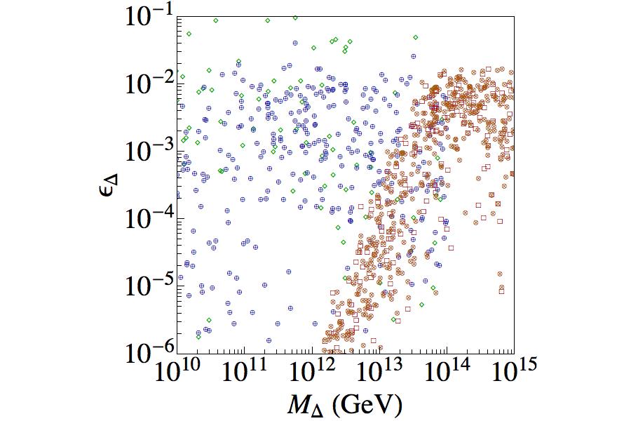
Figure 1: $\epsilon_{\Delta}$ as function of $M_{\Delta}$. Red squares and orange crosses for normal and inverted hierarchy of a specific 3-parameter predictive case. Green squares and blue crosses for normal and inverted hierarchy of the general 8-parameter case.

For illustration we present the results for the asymmetries of (2/$\mathds{I}$) in fig. 1 (red squares and orange crosses for normal and inverted hierarchy respectively).

Similarly non-vanishing asymmetries can be generated in the 3 parameter classes (1+$\mathds{I}$/1) and (1/1+$\mathds{I}$), due to the presence of $\mathds{I}$ and therefore of a non-vanishing $a_{0}^{X}$.

We turn finally to the special case of the minimal models (2/1) and (1/2) scenarios. For these the matrix $\boldsymbol{{\cal M}}$ must vanish as a consequence of the orthogonality of the $\boldsymbol{v_{i}}$ eigenvectors due to $\boldsymbol{Y}^{a}$ having the form $\boldsymbol{v_{k}}\otimes\boldsymbol{v_{k}}$ and the absence of repeated eigenvectors. This conclusion can be seen from eqs. (21), (22) and (23), (24) respectively: in either case we get two contributions: combining the single eigenvector of one seesaw type with the other two of the other seesaw type. The two contributions to $\boldsymbol{{\cal M}}$ necessarily share the matricial form constructed of orthogonal eigenvectors $\boldsymbol{v_{i}}^{T}.(\boldsymbol{v_{k}}\otimes\boldsymbol{v_{k}})^{\ast}.\boldsymbol{v_{i}}$ and individually vanish. This can also be seen explicitly by considering eq. (37) with $a_{0}^{I}=a_{0}^{II}=0$ and no repeated eigenvectors meaning $\sum_{i}\left(a_{i}^{I}a_{i}^{II\star}\right)=0$ with all individual terms in the sum vanishing (meaning $\epsilon_{\Delta}$ and all individual $\epsilon^{\Delta}_{N_{i}}$ vanish).

This result may appear to be incompatible with the leptogenesis discussion in [28] (where $\boldsymbol{{\cal M}}$ does not vanish despite having exact TB mixing). There is in fact no contradiction - the parametrisations used are both valid: here we consider one quite useful for studying hybrid leptogenesis, relying on the outer products $\boldsymbol{v_{k}}\otimes\boldsymbol{v_{k}}$;[28] relies on structures that simultaneously give insight into particular phenomenological consequences and have direct links to particular symmetries. If one takes a situation where the $\boldsymbol{Y}^{a}$ are proportional to the structures of [28] and re-express them into our eigenvector parametrisation, we readily conclude that such cases can lead to repeated eigenvectors, falling outside our minimal classes and therefore are able to produce non-vanishing asymmetries consistently with our analysis.

We conclude then that in these minimal classes as defined, even the interplay between type I and type II seesaw does not enable leptogenesis in the exact mixing limit. Leptogenesis becomes possible only when deviations from that limit are introduced (for example via the introduction of higher dimensional effective operators).

In fig. 1 we compare a predictive case governed by 3 parameters in red squares and orange crosses (in this case a (2/$\mathds{I}$)) against a general (3+$\mathds{I}$/3+$\mathds{I}$) case governed by 8 parameters in green squares and blue crosses. In fig. 2 we take the same (2/$\mathds{I}$) predictive case, present the values for the relevant $\epsilon^{\Delta}_{N_{i}}$ and compare the relative by taking their ratio $R_{\Delta}=\epsilon^{\Delta}_{N_{i}}/\epsilon_{\Delta}$.

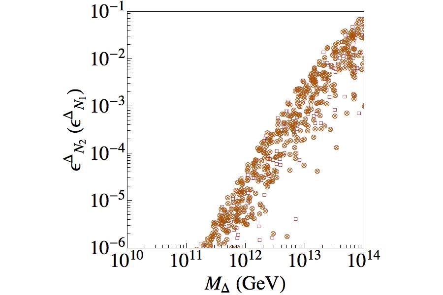
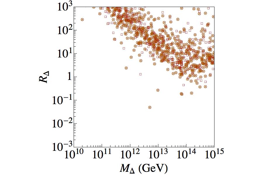
Figure 2: $\epsilon^{\Delta}_{N_{i}}$ (left-panel) and ratio $R_{\Delta}=\epsilon^{\Delta}_{N_{i}}/\epsilon_{\Delta}$ (right-panel) as function of $M_{\Delta}$ for a specific 3-parameter predictive case.

3.2 Generation of the $\boldsymbol{L}$ asymmetry

In a mixed scheme as the one we are discussing here, and assuming a hierarchical RH neutrino mass spectrum, leptogenesis can proceed in different ways according to the hierarchy between the mass of the lightest RH neutrino, $M_{N_{1}}$ and $M_{\Delta}$. If $M_{N_{1}}\ll M_{\Delta}$ the effects of $\boldsymbol{\Delta}$ are decoupled and the lepton asymmetry is generated via $N_{1}$ dynamics. Apart from the new contribution to the total CP asymmetry, eq. (26), there is no difference between this case and the standard leptogenesis scenario. Conversely, if $M_{N_{1}}\gg M_{\Delta}$ the lepton asymmetry is entirely produced by the dynamics of $\boldsymbol{\Delta}$. The triplet having non-trivial standard model quantum numbers couples to electroweak gauge bosons, so the determination of the lepton asymmetry, even at leading order in the couplings $\boldsymbol{Y}$, involves gauge boson induced triplet annihilations [19, 21]. One can also envisage a scenario where $\boldsymbol{\Delta}$ and $N_{1}$ being quasi-degenerate both generate the lepton asymmetry and this is the scenario we want to discuss in what follows.

In a hot plasma with $N$ lepton number and CP violating states $S_{1},\dots,S_{N}$ the evolution of the lepton asymmetry $L=\sum_{i=e,\mu,\tau}(2\ell_{i}+e_{i})$ ($e_{i}$ being the RH charged leptons) can be written, for a general mass spectrum, according to

$$\dot{Y}_{\Delta_{L}}(z)=\sum_{i=1}^{N}\dot{Y}^{(S_{i})}_{\Delta_{L}}(z)\,,$$ (43)

where, following ref. [29], we are using the notation $s(z)H(z)z\,d\,Y_{X}(z)/dz\equiv\dot{Y}_{X}(z)$. Here $z=M_{1}/T$ ($M_{1}$ being the mass of the lightest state), $Y_{\Delta_{X}}=n_{X}-n_{\bar{X}}/s$ with $n_{X}$ ($n_{\bar{X}}$) the number density of particles (antiparticles), $s$ the entropy density and $H(z)$ the expansion rate of the Universe (the definitions of these functions can be found in the appendix). $\dot{Y}_{\Delta_{L}}^{(S_{i})}(z)$ is the asymmetry generated by all the $N$ states. Note that in (43) we have written the dimensionless inverse temperature of the remaining states as $z_{i}=M_{i}/M_{1}\,z$.

In the case under consideration $N=2$ and the states correspond to the lightest $SU(2)$ singlet neutrino and scalar triplet, therefore

$$\dot{Y}_{\Delta_{L}}(z)=\dot{Y}_{\Delta_{L}}^{(N_{1})}(z)+\dot{Y}_{\Delta_{L}}^{(\Delta)}(z)\,.$$ (44)

At leading order in the couplings $\boldsymbol{\lambda}$ and $\boldsymbol{Y}$ i.e. ${\cal O}(\lambda^{2},Y^{2})$ the two pieces are given by

$$\dot{Y}_{\Delta_{L}}^{(N_{1})}(z) =\left(\dot{Y}_{\Delta_{L}}^{(N_{1})}(z)\right)_{1\leftrightarrow 2}+\left(\dot{Y}_{\Delta_{L}}^{(N_{1})}(z)\right)^{\text{sub}}_{2\leftrightarrow 2}\,,$$

$$\dot{Y}_{\Delta_{L}}^{(\Delta)}(z) =\left(\dot{Y}_{\Delta_{L}}^{(\Delta)}(z)\right)_{1\leftrightarrow 2}+\left(\dot{Y}_{\Delta_{L}}^{(\Delta)}(z)\right)^{\text{sub}}_{2\leftrightarrow 2}\,.$$ (45)

The first terms in the right-hand side ($1\leftrightarrow 2$) represent the contribution from the Yukawa induced decay and inverse decay processes, $N_{1}\leftrightarrow\ell\tilde{H}^{\dagger}$ and $\boldsymbol{\Delta}\leftrightarrow\bar{\ell}\bar{\ell}$; the second terms ($2\leftrightarrow 2$) the off-shell Yukawa generated scattering reactions $\ell\tilde{H}^{\dagger}\leftrightarrow\ell\tilde{H}^{\dagger}$ and $H^{\dagger}H^{\dagger}\leftrightarrow\ell\ell$, that even at leading order must be included so to obtain kinetic equations with the correct thermodynamical behaviour.

In addition to the evolution of the $Y_{\Delta_{L}}$ asymmetry the full network of Boltzmann equations should include the equations accounting for the evolution of the RH neutrino and triplet number densities and the triplet and Higgs asymmetries. A comment is in order: the Higgs asymmetry in most of the studies of standard leptogenesis is either neglected or treated as a spectator process [30], in the case in question -or in the pure triplet case- this in principle might be done if $\Gamma(\boldsymbol{\Delta}\to H\,H)\gg H(z)|_{z=1}$ can be guaranteed. This simplification, though possible, is not necessary as one out of the five equations governing the $L$ generation process can be removed by the condition imposed by hypercharge neutrality [21]:

$$2\,Y_{\Delta_{\Delta}}+Y_{\Delta H}-Y_{\Delta_{L}}=0\,.$$ (46)

With the above considerations the relevant system of kinetic equations can be written as

$$\dot{Y}_{N_{1}} = -(y_{N_{1}}-1)\,\gamma_{D_{N_{1}}}\,,$$

$$\dot{Y}_{\Sigma} = -(y_{\Sigma}-1)\,\gamma_{D_{\Delta}}-2(y_{\Sigma}^{2}-1)\,\gamma_{A}\,,$$

$$\dot{Y}_{\Delta_{L}} = \left[(y_{N_{1}}-1)\,\epsilon_{N_{1}}^{\text{tot}}-\left(y_{\Delta_{L}}+y_{\Delta_{\Delta}}^{H}\right)\right]\,\gamma_{D_{N_{1}}}$$

$$+\left[(y_{\Sigma}-1)\,\epsilon_{\Delta}-2K_{\ell}\,(y_{\Delta_{L}}+y_{\Delta_{\Delta}})\right]\,\gamma_{D_{\Delta}}\,,$$

$$\dot{Y}_{\Delta_{\Delta}} = -\left[y_{\Delta_{\Delta}}+(K_{\ell}-K_{H})\,y_{\Delta_{L}}+2K_{H}\,y_{\Delta_{\Delta}}^{H}\right]\,,$$ (47)

where the following conventions have been adopted: $y_{X}\equiv Y_{X}/Y_{X}^{\text{Eq}}$ (the exception being $y_{\Delta T}^{H}\equiv Y_{\Delta_{\Delta}}/Y_{H}^{\text{Eq}}$ and $y_{\Delta_{L}}=Y_{\Delta_{L}}/Y^{\text{Eq}}_{\ell}$), $\Sigma\equiv\Delta+\Delta^{\dagger}$, $\epsilon_{N_{1}}^{\text{tot}}\equiv\epsilon_{N_{1}}+\epsilon_{N_{1}}^{\Delta}$ and $\gamma_{D_{N_{1}}}$, $\gamma_{D_{\Delta}}$ and $\gamma_{A}$ are the reaction densities for: RH neutrino and triplet decays and triplet annihilations (expressions for these quantities are given in the appendix). The factors $K_{\ell,H}$ resemble the flavor projectors defined in standard flavored leptogenesis [31, 32] as they project triplet decays into either the Higgs or the lepton doublet directions. They are defined as follows

$$K_{\ell}=\frac{\tilde{m}_{\Delta}^{\ell}}{\tilde{m}_{\Delta}^{\ell}+\frac{\tilde{m}_{\Delta}^{2}}{4\,\tilde{m}_{\Delta}^{\ell}}}\,\qquad\mbox{and}\qquad K_{H}=\frac{\tilde{m}_{\Delta}^{2}}{4\,\tilde{m}_{\Delta}^{\ell}\left(\tilde{m}_{\Delta}^{\ell}+\frac{\tilde{m}_{\Delta}^{2}}{4\,\tilde{m}_{\Delta}^{\ell}}\right)}\,,$$ (48)

where the parameters $\tilde{m}_{\Delta}^{\ell}$ and $\tilde{m}^{2}_{\Delta}$ are given by

$$\tilde{m}_{\Delta}^{\ell}=\frac{v^{2}\,|\boldsymbol{Y}|^{2}}{M_{\Delta}}\qquad\mbox{and}\qquad\tilde{m}^{2}_{\Delta}=\mbox{Tr}[\boldsymbol{m_{\nu}^{II}}\boldsymbol{m_{\nu}^{II}}^{\dagger}]\,,$$ (49)

with $|\boldsymbol{Y}|^{2}=\mbox{Tr}[\boldsymbol{Y}\,\boldsymbol{Y}^{\dagger}]$. In these definitions we have replaced the trilinear coupling $\mu$ by the contribution of the type-II sector to the effective light neutrino mass matrix, encoded in $\tilde{m}^{2}_{\Delta}$. In principle this is just a matter of choice, but it proves to be quite convenient given that in contrast to $\mu$ the parameter $\tilde{m}_{\Delta}$ is (partially) constrained by experimental neutrino data.

As we have already stressed the scenario we consider here is defined by a hierarchical RH neutrino mass spectrum and a mild hierarchy between $M_{N_{1}}$ and $M_{\Delta}$, that we choose to be in the range $10^{-1}\lesssim M_{\Delta}/M_{N_{1}}\lesssim 1$. Consequently, as explained at the beginning of this section $z=M_{\Delta}/T$ and $z_{N}=r\,z$ with $r=M_{N_{1}}/M_{\Delta}$. In that way, once the CP asymmetries in both sectors (I and II) are specified, the problem of studying the evolution of the $L$ asymmetry is completely determined by five parameters: the contribution of the lightest RH neutrino to light neutrino masses $\tilde{m}_{N_{1}}=v^{2}(\boldsymbol{\lambda}\boldsymbol{\lambda}^{\dagger})_{11}/M_{N_{1}}$, $\tilde{m}_{\Delta}$, $\tilde{m}_{\Delta}^{\ell}$, $M_{\Delta}$ and $r$ .

Assuming an initial vanishing $L$ asymmetry ($Y_{\Delta_{L}}(z\to 0)=0$), the formal solution of the differential equation governing this asymmetry in eq. (3.2) yields

$$Y_{\Delta_{L}}(z)=\int_{z_{i}}^{z}\,dz^{\prime}\,P(z^{\prime})\,e^{-\int_{z^{\prime}}^{z}\,dz^{\prime\prime}\,Q(z^{\prime\prime})}\,,$$ (50)

with the functions $P(z)=P^{I}(z)+P^{II}(z)$ and $Q(z)$ given by

$$P^{I}(z) =\frac{1}{s(z)H(z)z}\left\{\left[(y_{N_{1}}(z)-1)\epsilon_{N_{1}}^{\text{tot}}-y_{\Delta_{\Delta}}^{H}(z)\right]\gamma_{D_{N_{1}}}(z)\right\}\,,$$ (51)

$$P^{II}(z) =\frac{3}{s(z)H(z)z}\left\{\left[(y_{\Sigma}(z)-1)\epsilon_{\Delta}-2K_{\ell}\,y_{\Delta_{\Delta}}(z)\right]\gamma_{D_{\Delta}}(z)\right\}\,,$$ (52)

$$Q(z) =\frac{1}{s(z)H(z)z}\left[\frac{1}{Y^{\text{Eq}}_{\ell}}\left(\gamma_{D_{N_{1}}}(z)+2\,K_{\ell}\,\gamma_{D_{\Delta}}(z)\right)\right]\,.$$ (53)

Note that in $P^{II}(z)$ we have included a factor of 3 coming from the triplet $SU(2)$ physical degress of freedom. By factorizing either $\epsilon_{N_{1}}^{\text{tot}}$ or $\epsilon_{\Delta}$ from the functions $P^{I,II}(z)$ and normalizing to $Y^{\text{Eq}}_{\text{tot}}\equiv Y^{\text{Eq}}_{\text{tot}}(z\to 0)=Y^{\text{Eq}}_{N_{1}}(z)+Y^{\text{Eq}}_{\Sigma}(z)|_{z\to 0}$ the $L$ asymmetry in (50) can be written in terms of efficiency functions that depend on the dynamics of the scalar triplet and the fermionic singlet, namely

$$Y_{\Delta_{L}}(z)=-\epsilon_{N_{1}}^{\text{tot}}\,Y^{\text{Eq}}_{\text{tot}}\,\eta^{I}(z)\quad\mbox{and}\quad Y_{\Delta_{L}}(z)=-\epsilon_{\Delta}\,Y^{\text{Eq}}_{\text{tot}}\,\eta^{II}(z)\,.$$ (54)

The functions $\eta^{I,II}(z)$ are defined in such a way that in the limit in which the triplet (RH neutrino) interactions are absent $\eta^{I}$ ($\eta^{II}$) corresponds to the efficiency function of standard leptogenesis (pure triplet leptogenesis). As usual the final $L$ asymmetry is obtained from these functions in the limit $z\to\infty$.

In models with an interplay of type I and II seesaws exhibiting a mild hierarchy between the $\Delta$ and $N_{1}$ masses several scenarios for the generation of the lepton asymmetry can be considered:

1. Purely triplet scalar leptogenesis models:
   The relevant parameters follow the hierarchy $\tilde{m}_{N_{1}}\ll\tilde{m}_{\Delta}^{\ell},\tilde{m}_{\Delta}$. The $L$ asymmetry is generated through the processes $\boldsymbol{\Delta}\to\bar{\ell}\bar{\ell}$ or $\boldsymbol{\Delta}\to HH$ and the details strongly depend on whether $\tilde{m}_{\Delta}^{\ell}\gg\tilde{m}_{\Delta}$, $\tilde{m}_{\Delta}^{\ell}\ll\tilde{m}_{\Delta}$ or $\tilde{m}_{\Delta}^{\ell}\sim\tilde{m}_{\Delta}$. Interestingly, when $\tilde{m}_{\Delta}^{\ell}\gg\tilde{m}_{\Delta}$ the Higgs asymmetry -being weakly washed out- turns out to be large and implies a large lepton asymmetry.

   In order to illustrate how leptogenesis proceeds in these models we have solved the network of Boltzmann equations in (3.2) for the benchmark point $P_{I}$=($\tilde{m}_{N_{1}}$, $\tilde{m}_{\Delta}$, $\tilde{m}_{\Delta}^{\ell}$,$M_{\Delta}$,$r$) =($10^{-4}$ eV, $10^{-2}$ eV, $10^{-1}$ eV, $10^{10}$ GeV,2) for fixed $\epsilon_{\Delta}=10^{-6}$ and $\epsilon_{N_{1}}=10^{-5}$ and assuming initial vanishing asymmetries. The results are displayed in fig. 3. With this parameter choice the generation of the $L$ is entirely determined by the triplet reactions. As can be seen in fig. 3 (left-panel) the RH neutrino reaction density is tiny implying in the equation for the evolution of the $L$ asymmetry in (3.2) the RH related quantities can be neglected. For the triplet-Higgs reaction density $\gamma_{D_{\Delta}}^{H}$, though also small, this is not the case: the relevant reaction density in the pure type II sector is $\gamma_{D_{\Delta}}=\gamma_{D_{\Delta}}^{H}+\gamma_{D_{\Delta}}^{\ell}$ so due to the constraint $\gamma_{D_{\Delta}}^{H}\ll\gamma_{D_{\Delta}}^{\ell}$ the Higgs asymmetry does not suffers from a strong washout ($K_{H}\sim 10^{-3}$) and becomes large. Due to the hypercharge neutrality condition, eq. (46), a large lepton and triplet asymmetry develops. Once the triplet number density starts being diluted, due to decays controlled by $\gamma_{D_{\Delta}}^{\ell}$, the asymmetry stored in triplets is transferred to the lepton asymmetry. This can be observed in fig. 3 (right-panel) where at $z\sim 5$ the triplet asymmetry drops and the $Y_{\Delta_{L}}$ increases accordingly. The situation described here is quite similar to what happens in standard flavored leptogenesis [31, 32, 33] where, depending on the lepton flavor projectors, a large asymmetry in a particular flavor can be stored yielding in turn a large net lepton asymmetry.

   

   

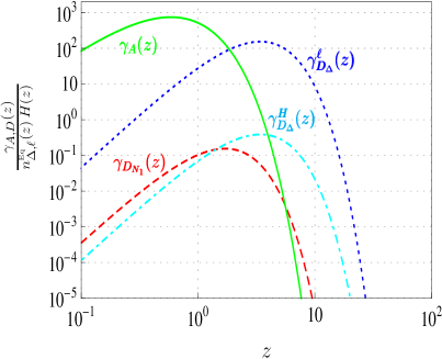
   Figure 3: Reaction densities for triplet and RH neutrino processes (left-panel) and evolution of the different densities (right-panel) entering in the kinetic equations for the scenario of purely triplet leptogenesis. See the text for more details.

2. Singlet dominated leptogenesis models:
   These scenarios are defined according to $\tilde{m}_{N_{1}}\gg\tilde{m}_{\Delta}^{\ell},\tilde{m}_{\Delta}$ thus leptogenesis is mainly determined by $N_{1}$ dynamics. The relative difference between the parameters $\tilde{m}_{\Delta}^{\ell}$ and $\tilde{m}_{\Delta}$ determines whether either the Higgs asymmetry or the $L$ asymmetry are strongly or weakly washed out, thus three cases can be distinguished: $\tilde{m}_{\Delta}^{\ell}\gg\tilde{m}_{\Delta}$, $\tilde{m}_{\Delta}^{\ell}\ll\tilde{m}_{\Delta}$ or $\tilde{m}_{\Delta}^{\ell}\sim\tilde{m}_{\Delta}$. Each of them exhibit different features.

   

   

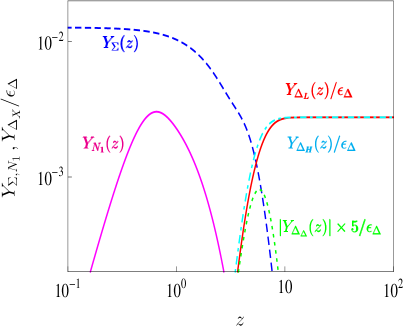
   Figure 4: Reaction densities for triplet and RH neutrino processes (left-panel) and evolution of the different densities (right-panel) entering in the kinetic equations for the scenario of singlet dominated leptogenesis. See the text for more details.

   We have solved eqs. (3.2) for the case $\tilde{m}_{\Delta}^{\ell}\gg\tilde{m}_{\Delta}$ by fixing the parameter space point $P_{II}$=($\tilde{m}_{N_{1}}$, $\tilde{m}_{\Delta}$, $\tilde{m}_{\Delta}^{\ell}$,$M_{\Delta}$,$r$) =($10^{-2}$ eV, $10^{-4}$ eV, $10^{-3}$ eV, $10^{10}$ GeV,2) with the CP asymmetries $\epsilon_{N_{1}}^{\text{tot}},\epsilon_{\Delta}$ settled as in the previous analysis. The results are displayed in figure 4 (right-panel). Due to the hierarchy $\gamma_{D_{N_{1}}}\gg\gamma_{D_{\Delta}}^{\ell,H}$ (see fig. 4 (left-panel)) the triplet asymmetry is tiny. The hypercharge neutrality condition thus implies almost exact $L$ and Higgs asymmetries, the deviations determined by the small amount of $Y_{\Delta_{\Delta}}$ produced. Compared with the models discussed in the previous item in this case $Y_{\Sigma}$ departs from thermal equilibrium at higher temperatures (smaller values of $z$), the decoupling temperature entirely determined by gauge reaction decoupling ($\gamma_{A}(z)/(n_{\Delta}^{\text{Eq}}(z)H(z))<1$) . For the example in figure 4 it can be seen this happens at $z\sim 5$, the small bump in $Y_{\Sigma}(z)$ is actually due to this effect.

3. Mixed leptogenesis models:
   In these models the parameters controlling gauge reactions strengths are all of the same order i.e. $\tilde{m}_{N_{1}}\sim\tilde{m}_{\Delta}^{\ell}\sim\tilde{m}_{\Delta}$, so drawing general conclusions from the analysis of particular benchmark points is far more involved and the general picture may only be obtained by scans of the relevant parameters. However, with the purpose of highlighting some of the aspects of these schemes we have solved the set of eqs. in (3.2) assuming $P_{III}$=($\tilde{m}_{N_{1}}$, $\tilde{m}_{\Delta}$, $\tilde{m}_{\Delta}^{\ell}$,$M_{\Delta}$,$r$) =($2\times 10^{-2}$ eV, $4\times 10^{-2}$ eV, $6\times 10^{-2}$ eV, $10^{10}$ GeV,2) with $\epsilon_{N_{1}}^{\text{tot}}$ and $\epsilon_{\Delta}$ fixed as in the previous two analyses. The results are shown in fig. 5, we have not included in this case neither the $\Sigma$ nor the $N_{1}$ abundances as the former behaves as in purely triplet leptogenesis models while the later as in singlet dominated ones. It can be seen that due to the parameter choice $\gamma_{D_{\Delta}}^{\ell,H}$ overcome the corresponding gauge reactions at $z\sim 3$ maintaining the $Y_{\Sigma}$ abundance close to the equilibrium distribution. The total $L$ asymmetry is two orders of magnitude smaller than in the purely triplet and singlet dominated leptogenesis models we have considered, in part because the washouts in both the Higgs and lepton directions are large ($K_{\ell}=0.64$, $K_{H}=0.36$) but it remains to be seen whether this is a general feature of these type of models.

   

   

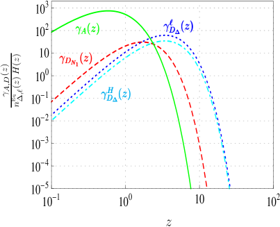
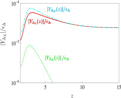
   Figure 5: Reaction densities for triplet and RH neutrino processes (left-panel) and evolution of the different densities (right-panel) entering in the kinetic equations for mixed leptogenesis models. See the text for more details.

4 Conclusions

We have studied leptogenesis in models featuring the interplay between type I and type II seesaw in the presence of flavor symmetries. By assuming an exact mixing scheme we classified in a model independent way the possible realizations of such hybrid scenarios. The possible models can be grouped according to whether in the limit of exact mixing the CP violating asymmetry $\epsilon_{N}$ vanishes or not. Our results show that the presence of additional degrees of freedom may allow viable leptogenesis without requiring any departure from exact mixing, particularly for non-minimal models that can include the identity matrix (according to the definition of minimal in sec. 2). Effectively, only the repetition of eigenvectors across both seesaws can produce a contribution and if no eigenvectors are repeated the asymmetry must vanish - however the identity matrix counts as all eigenvectors so its presence on one of the seesaws automatically repeats any present in the other. In the case of minimal models the constraints imposed by exact mixing enforce a vanishing CP violating asymmetry, thus resembling the results of flavor models based just on type I seesaw.

As regards the generation of the lepton asymmetry we have shown that by going beyond the limit of RH neutrino decoupling, allowing the RH neutrino and triplet mass splitting to be small, permits a variety of scenarios for leptogenesis. We have done an analysis of these realizations for particular benchmark points in the relevant parameter space. Our results show these models exhibit different qualitative as well as quantitative features that may lead leptogenesis to be quite different from the standard picture.

Although based on the TB mixing scheme -for concreteness- our conclusions remain valid regardless of the mixing pattern, provided the flavor symmetry enforces the type I and type II light neutrino mass matrices to be form-diagonalizable. Accordingly, our findings constitute a new pathway to leptogenesis in models in which a flavor symmetry is responsible for lepton mixing.

5 Acknowledgments

We would like to thank Stefan Antusch for helpful comments. DAS is supported by a Belgian FNRS postdoctoral fellowship. IdMV is supported by DFG grant PA 803/6-1.

Appendix A Notation and conventions

In this appendix we fix the conventions that have been used in sec. 3.2 for the discussion of the different leptogenesis realizations one can define in models featuring an interplay between type I and II seesaws and a mild hierarchy between the electroweak triplet scalar and the lightest RH neutrino.

We have used Maxwell-Boltzmann distribution functions for massless (relativistic) as well as massive species:

$$n_{\Delta}^{\text{Eq}}(z)=\frac{3\,M_{\Delta}^{3}}{2\,\pi^{2}}\,\frac{K_{2}(z)}{z}\,,\quad n_{N_{1}}^{\text{Eq}}(z)=\frac{M_{\Delta}^{3}}{\pi^{2}}\,r^{2}\frac{K_{2}(r\,z)}{z}\,,\quad n_{\ell,H}^{\text{Eq}}(z)=\frac{2}{\pi^{2}}\,\frac{M_{\Delta}^{3}}{z}\,,$$ (55)

where, as mentioned in sec. 3.2, $r=M_{N_{1}}/M_{\Delta}$ and $K_{n}(z)$ is the $n$-th order modified Bessel function of the second type. The entropy density and the expansion rate of the Universe are defined as usual, namely

$$s(z)=\frac{4\,g_{*}}{\pi^{2}}\frac{M_{\Delta}^{3}}{z^{3}}\,,\quad H(z)=\sqrt{\frac{8g_{*}}{\pi}}\frac{M_{\Delta}^{2}}{M_{\text{Planck}}}\frac{1}{z^{2}}$$ (56)

with the number of relativistic degrees of freedom given by $g_{*}=118$ and the Planck mass by $M_{\text{Planck}}=1.22\times 10^{19}$ GeV.

The reaction densities for $1\leftrightarrow 2$ processes are given by

$$\gamma_{D_{N_{1}}}(z) =\frac{1}{8\,\pi^{3}}\frac{M_{\Delta}^{5}}{v^{2}}r^{4}\frac{K_{1}(rz)}{z}\,\tilde{m}_{N_{1}}\,,$$

$$\gamma_{D_{\Delta}}^{H}(z) =\frac{1}{8\,\pi^{3}}\frac{M_{\Delta}^{5}}{v^{2}}\frac{K_{1}(z)}{z}\,\frac{\tilde{m}_{\Delta}^{2}}{4\tilde{m}_{\Delta}^{\ell}}\,,$$

$$\gamma_{D_{\Delta}}^{\ell}(z) =\frac{1}{8\,\pi^{3}}\frac{M_{\Delta}^{5}}{v^{2}}\frac{K_{1}(z)}{z}\,\tilde{m}_{\Delta}^{\ell}\,,$$ (57)

where the full triplet reaction density is given by $\gamma_{D_{\Delta}}=\gamma_{D_{\Delta}}^{H}+\gamma_{D_{\Delta}}^{\ell}$. For $2\leftrightarrow 2$ triplet annihilations the corresponding reaction density reads

$$\gamma_{A}(z)=\frac{M_{\Delta}^{4}}{64\,\pi^{4}}\,\int_{4}^{\infty}dx\sqrt{x}\frac{K_{1}(zx)}{z}\,\widehat{\sigma}_{A}(x)\,,$$ (58)

where $x=s/M_{\Delta}^{2}$. The reduced cross section $\widehat{\sigma}_{A}(x)=2\,x\,\lambda(1,x^{-1},0)$ (where we have $\lambda(a,b,c)=(a-b-c)^{2}-4bc$) and involves the $s$-channel processes $\boldsymbol{\Delta}\boldsymbol{\Delta}\to F\bar{F},AA,HH$ ($F$ and $A$ stand for standard model fermions and $SU(2)\times U(1)$ gauge bosons respectively), $t$ and $u$ channel triplet mediated processes $\boldsymbol{\Delta}\boldsymbol{\Delta}\to AA$ and the “quartic” process $\boldsymbol{\Delta}\boldsymbol{\Delta}\to AA$. In powers of the kinematic factor $\omega(x)=\sqrt{1-4/x}$ it can be split in three pieces [21]:

$$\widehat{\sigma}_{1}(x) =\frac{1}{\pi}\left[g^{4}\left(5+\frac{34}{x}\right)+\frac{3}{2}g^{\prime 4}\left(1+\frac{4}{x}\right)\right]\omega(x)\,,$$

$$\widehat{\sigma}_{2}(x) =\frac{1}{8\pi}\left(25g^{4}+\frac{41}{2}g^{\prime 4}\right)\omega(x)^{3}\,,$$

$$\widehat{\sigma}_{3}(x) =\frac{6}{\pi x^{2}}\left[4g^{4}(x-1)+g^{\prime 4}(x-2)\right]\ln\left[\frac{1+\omega(x)}{1-\omega(x)}\right]\,,$$ (59)

with $\widehat{\sigma}_{A}(x)=\sum_{i=1}^{3}\widehat{\sigma}_{i}(x)$ and $g,g^{\prime}$ the $SU(2)$ and $U(1)$ gauge couplings.

References

- [1] P. Minkowski, Phys. Lett. B 67 421 (1977); T. Yanagida, in Proc. of Workshop on Unified Theory and Baryon number in the Universe, eds. O. Sawada and A. Sugamoto, KEK, Tsukuba, (1979) p.95; M. Gell-Mann, P. Ramond and R. Slansky, in Supergravity, eds P. van Niewenhuizen and D. Z. Freedman (North Holland, Amsterdam 1980) p.315; P. Ramond, Sanibel talk, retroprinted as hep-ph/9809459; S. L. Glashow, inQuarks and Leptons, Cargèse lectures, eds M. Lévy, (Plenum, 1980, New York) p. 707; R. N. Mohapatra and G. Senjanović, Phys. Rev. Lett. 44, 912 (1980); J. Schechter and J. W. F. Valle, Phys. Rev. D 22 (1980) 2227; Phys. Rev. D 25 (1982) 774.
- [2] J. Schechter and J. W. F. Valle, Phys. Rev. D 22, 2227 (1980); G. Lazarides, Q. Shafi and C. Wetterich, Nucl. Phys. B 181, 287 (1981); R. N. Mohapatra and G. Senjanovic, Phys. Rev. D 23, 165 (1981); C. Wetterich, Nucl. Phys. B 187, 343 (1981);
- [3] R. Foot, H. Lew, X. G. He and G. C. Joshi, Z. Phys. C 44, 441 (1989).
- [4] S. Davidson, E. Nardi and Y. Nir, Phys. Rept. 466, 105 (2008) [arXiv:0802.2962 [hep-ph]].
- [5] G. L. Fogli, E. Lisi, A. Marrone, A. Palazzo and A. M. Rotunno, Phys. Rev. D 84, 053007 (2011) [arXiv:1106.6028 [hep-ph]].
- [6] T. Schwetz, M. Tortola, J. W. F. Valle, [arXiv:1108.1376 [hep-ph]].
- [7] G. Altarelli, F. Feruglio, Rev. Mod. Phys. 82 (2010) 2701-2729. [arXiv:1002.0211 [hep-ph]].
- [8] E. E. Jenkins, A. V. Manohar, Phys. Lett. B668, 210-215 (2008). [arXiv:0807.4176 [hep-ph]].
- [9] C. Hagedorn, E. Molinaro, S. T. Petcov, JHEP 0909, 115 (2009). [arXiv:0908.0240 [hep-ph]].
- [10] E. Bertuzzo, P. Di Bari, F. Feruglio, E. Nardi, JHEP 0911, 036 (2009). [arXiv:0908.0161 [hep-ph]].
- [11] D. Aristizabal Sierra, F. Bazzocchi, I. de Medeiros Varzielas, L. Merlo, S. Morisi, Nucl. Phys. B827, 34-58 (2010). [arXiv:0908.0907 [hep-ph]].
- [12] R. G. Felipe, H. Serodio, Phys. Rev. D81, 053008 (2010). [arXiv:0908.2947 [hep-ph]].
- [13] D. Aristizabal Sierra, M. Losada, E. Nardi, Phys. Lett. B659, 328-335 (2008). [arXiv:0705.1489 [hep-ph]].
- [14] D. Aristizabal Sierra, L. A. Munoz, E. Nardi, Phys. Rev. D80, 016007 (2009). [arXiv:0904.3043 [hep-ph]].
- [15] D. Aristizabal Sierra, F. Bazzocchi, [arXiv:1110.3781 [hep-ph]].
- [16] I. K. Cooper, S. F. King and C. Luhn, arXiv:1110.5676 [hep-ph].
- [17] E. K. Akhmedov, M. Frigerio, JHEP 0701, 043 (2007). [hep-ph/0609046].
- [18] T. Hambye, G. Senjanovic, Phys. Lett. B582, 73-81 (2004). [hep-ph/0307237].
- [19] T. Hambye, Y. Lin, A. Notari, M. Papucci, A. Strumia, Nucl. Phys. B695, 169-191 (2004). [hep-ph/0312203].
- [20] S. Antusch and S. F. King, Phys. Lett. B 597, 199 (2004) [hep-ph/0405093].
- [21] T. Hambye, M. Raidal, A. Strumia, Phys. Lett. B632, 667-674 (2006). [hep-ph/0510008].
- [22] S. Antusch, Phys. Rev. D 76, 023512 (2007) [arXiv:0704.1591 [hep-ph]].
- [23] S. -L. Chen, M. Frigerio, E. Ma, Nucl. Phys. B724, 423-431 (2005). [arXiv:hep-ph/0504181 [hep-ph]].
- [24] C. I. Low, R. R. Volkas, Phys. Rev. D68, 033007 (2003). [hep-ph/0305243].
- [25] S. F. King, JHEP 0508, 105 (2005). [hep-ph/0506297].
- [26] I. de Medeiros Varzielas, G. G. Ross, Nucl. Phys. B733, 31-47 (2006). [hep-ph/0507176].
- [27] S. Antusch and S. F. King, JHEP 0601, 117 (2006) [hep-ph/0507333].
- [28] I. de Medeiros Varzielas, R. Gonzalez Felipe, H. Serodio, Phys. Rev. D83, 033007 (2011). [arXiv:1101.0602 [hep-ph]].
- [29] E. Nardi, J. Racker, E. Roulet, JHEP 0709, 090 (2007). [arXiv:0707.0378 [hep-ph]].
- [30] E. Nardi, Y. Nir, J. Racker and E. Roulet, JHEP 0601, 068 (2006) [hep-ph/0512052].
- [31] E. Nardi, Y. Nir, E. Roulet and J. Racker, JHEP 0601, 164 (2006) [hep-ph/0601084].
- [32] A. Abada, S. Davidson, A. Ibarra, F. -X. Josse-Michaux, M. Losada and A. Riotto, JHEP 0609, 010 (2006) [hep-ph/0605281].
- [33] R. Barbieri, P. Creminelli, A. Strumia and N. Tetradis, Nucl. Phys. B 575, 61 (2000) [hep-ph/9911315].