Convex Multiclass Segmentation with Shearlet Regularization
Abstract
Segmentation plays an important role in many preprocessing stages in image processing. Recently, convex relaxation methods for image multi-labeling were proposed in the literature. Often these models involve the total variation (TV) semi-norm as regularizing term. However, it is well-known that the TV functional is not optimal for the segmentation of textured regions. In recent years directional representation systems were proposed to cope with curved singularities in images. In particular, curvelets and shearlets provide an optimally sparse approximation in the class of piecewise smooth functions with singularity boundaries. In this paper, we demonstrate that the discrete shearlet transform is suited as regularizer for the segmentation of curved structures. Neither the shearlet nor the curvelet transform where used as regularizer in a segmentation model so far. To this end, we have implemented a translation invariant finite discrete shearlet transform based on the FFT. We describe how the shearlet transform can be incorporated within the multi-label segmentation model and show how to find a minimizer of the corresponding functional by applying an alternating direction method of multipliers. Here the Parseval frame property of our shearlets comes into play. We demonstrate by numerical examples that the shearlet regularized model can better segment curved textures than the TV regularized one and that the method can also cope with regularizers obtained from non-local means.
1 Introduction
In recent years, much effort has been spent to design directional representation systems for images such as curvelets [8], ridgelets [9] and shearlets [28] and corresponding transforms (this list is not complete). Among these transforms, the shearlet transform stands out since it stems from a square-integrable group representation [13] and has the corresponding useful mathematical properties. Moreover, similarly as wavelets are related to Besov spaces via atomic decompositions, shearlets correspond to certain function spaces, the so-called shearlet coorbit spaces [14]. In addition shearlets provide an optimally sparse approximation in the class of piecewise smooth functions with singularity curves, i.e.,
where is the nonlinear shearlet approximation of a function from this class obtained by taking the largest shearlet coefficients in absolute value.
In the following, we want to show how the directional information encoded by the shearlet transform can be used in image segmentation. Although shearlets and curvelets have been applied to a wide field of image processing tasks, see, e.g., [22, 29, 30, 35, 36, 45], to the best of our knowledge they were not used in connection with segmentation so far. Segmentation is a fundamental task in image processing which plays a role in many preprocessing steps. Recently, convex relaxation methods for image multi-labeling were addressed by several authors [2, 16, 26, 27, 32, 33, 34, 39, 41, 47]. In these methods a convex functional consisting of a data term and a regularization term is minimized. Due to its edge-preserving properties a frequent choice for the regularization term is the total variation (TV) semi-norm introduced by Rudin, Osher and Fatemi [40]. The data term is either related to a predefined codebook (of gray/RGB-values related to the labels) or the codebook is updated during the minimization process itself. For the later approach see, e.g., [3, 11, 25]. In this paper, we focus on the first approach, but replace the TV regularizer by the shearlet transform. To this end, we introduce a simple discrete shearlet transform which translates the shearlets over the full grid at each scale and for each direction. Using the FFT this transform can be still realized in a fast way. We show by numerical examples that the shearlet regularized model is well-suited to segment curved textures and can even cope with models incorporating nonlocal means.
for and
This paper is organized as follows: In Section 2 we introduce the translation invariant, finite, discrete shearlet transform whose full description cannot be found in the literature so far. Here we follow the path via the continuous shearlet transform, its counterpart on cones and finally its discretization on the full grid. This is different to other implementations as, e.g., in ShearLab111http://www.shearlab.org, see [43]. Our discrete shearlet transform can be efficiently computed by the fast Fourier transform (FFT). The discrete shearlets constitute a Parseval frame of the finite Euclidean space such that the inversion of the shearlet transform can be simply done by applying the adjoint transform. This is proven in Theorem 2.2 and cannot be found in the literature so far. In Section 3 we recall a convex multi-label segmentation model and show how the shearlet transform can be incorporated into this approach. We propose the method of alternating direction of multipliers (ADMM) [4, 15, 17, 18] to find a minimizer of the functional where the Parseval frame property of our shearlet frame can be exploited. Numerical results are presented in Section 4, in particular in comparison with models involving TV and nonlocal means (NL) regularizers [6, 19, 20, 44].
2 Finite Discrete Shearlet Transform
We start with a brief introduction of the finite discrete shearlet transform to make the paper self-contained. First we describe the continuous shearlet transform in and on cones. Then we provide a discretization of the shearlet transform on a finite domain which is translation invariant and cannot be found in this way in the literature. We prove that the discrete shearlets constitute a Parseval frame of the finite Euclidean space so that the inversion of the shearlet transform can be simply done by applying its adjoint transform. For a more detailed description we refer to [24].
Continuous Shearlets.
Let the parabolic scaling matrix and the shear matrix be defined by
Then the continuous shearlets emerge by dilation, shearing and translation of a function as
| (1) |
see [28, 31]. Using the Fourier transform given by
we obtain that
The continuous shearlet transform of a function is defined by
The shearlet transform is invertible if the function fulfills the admissibility property
This is in particular the case if
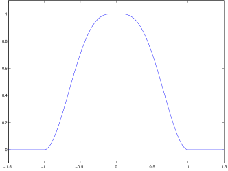
where is a wavelet and a bump function. Typical choices for these functions are
| (2) |
where
and
were introduced by Y. Meyer [38, 37]. The functions and are shown in Fig. 2. It is well-known that they have the following useful properties.
Lemma 2.1.
The functions and defined by (2) fulfill
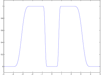
with (right).
Shearlets on Cones.
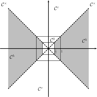
To get a good directional selectivity both from the horizontal and vertical point of view shearlets on the cone were introduced in [28]. We define the horizontal and the vertical cone by
resp., and the “intersection” (seam lines) of the two cones and the “low frequency” set by
resp., see Fig. 3. Altogether with an overlapping domain .
For each set , we define a characteristic function which is equal to 1 for and 0 otherwise. The shearlets on the cone are defined by
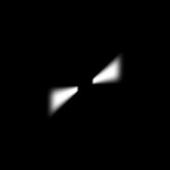
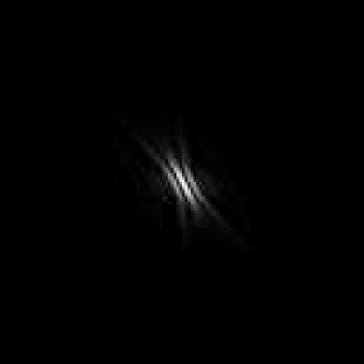
Fig. 4 shows shearlets both in the time and frequency domain. Note that for we have and for parts of are also in which are cut off. For the whole shearlets are set to zero by the characteristic function. For , i.e. , we define Finally, we use the scaling function defined by
with
and its translates , i.e., on . Note that this scaling function (respectively ) matches perfectly with , more precisely, since
we obtain
| (3) |
Finite Discrete Shearlets.
In the following, we consider digital images as functions sampled on the grid , where we assume quadratic images for simplicity. Further, let be the number of considered scales. To obtain a discrete shearlet transform, we discretize the scaling, shear and translation parameters as
With these notations our shearlets becomes . Observe that compared to the continuous shearlets defined in (1) we omit the factor . In the Fourier domain we obtain
where
for and
By definition we have and . Therefore we see that we have a cut off due to the cone boundaries only for where . For both cones we have for two “half” shearlets with a gap at the seam line. None of the shearlets are defined on the seam line . To obtain “full” shearlets at the seam lines we “glue” the three parts together, thus, we define for a sum of shearlets
We define the discrete shearlet transform as
where , and if not stated in another way. The shearlet transform can be efficiently realized by applying the fft2 and its inverse ifft2 which compute the following discrete Fourier transforms with arithmetic operations:
We have the Plancherel formula
Thus, the discrete shearlet transform can be computed for as follows:
| (4) | ||||
and with the corresponding modifications for .
In view of the inverse shearlet transform we prove that our discrete shearlets constitute a Parseval frame of the finite Euclidean space . Recall that for a Hilbert space a sequence is a frame if and only if there exist constants such that
The frame is called tight if and a Parseval frame if . For Parseval frames the reconstruction formula
holds true, see [12, 37]. In the -dimensional Euclidean space we can arrange the frame elements , as rows of a matrix . Then we have indeed a frame if has full rank and a Parseval frame if and only if . Note that is only true if the frame is an orthonormal basis. The Parseval frame transform and its inverse read
| (5) |
By the following theorem our shearlets provide such a convenient system.
Theorem 2.2.
The discrete shearlet system
provides a Parseval frame for .
Proof.
We have to show that
By (4) we know that
so that by Parseval’s formula
Analogous computations can be done for the vertical cone, the seam-line part and the low-pass part, see [24]. Summing up the different pieces we obtain
which can be further simplified by Lemma 2.1 as
Finally we obtain by (3) that
and we are done. ∎
Having a Parseval frame the inverse shearlet transform reads
The actual computation of from given coefficients is done in the Fourier domain. Due to the linearity of the Fourier transform we get, e.g., for the horizontal cone
The inner sum can be interpreted as a two-dimensional discrete Fourier transform and can be computed via a FFT. Hence, can be computed by simple multiplications of these Fourier-transformed shearlet coefficients with the dilated and sheared spectra of and afterwards summing over all scales and all shears . The spectra are the same as for the transform itself and can be reused. Finally we get itself by an iFFT of . For implementation details we refer to [24].
Remark 2.3.
1. We are aware of our larger oversampling factor in comparison with, e.g., ShearLab. Having 4 scales we obtain 61 images of the same size as the original image. But since shearlets are designed to detect edges in images we like to avoid any down-sampling and keep translation invariance. A possibility to reduce the memory usage would be to use the compact support of the shearlets in the frequency domain and only compute them on a “relevant” region. But we then would also have to store the position and size of each region what decreases the memory savings and would make the implementation a lot more complicated.
2. In [43] and the respective implementation ShearLab a pseudo-polar Fourier-transform is used to implement a discrete (or digital) shearlet transform. For the scale and the shear the same discretization is used. But for the translation the authors set . Thus, their discrete shearlet becomes
Since the operation would destroy the pseudo-polar grid a “slight” adjustment is made and the exponential term is replaced by
with and such that
With this adjustment the last step of the shearlet transform can be obtained with a standard inverse fast Fourier transform (similar as in our implementation). Unfortunately this is no longer related to translations of the shearlets in the time domain.
3. Having a look at the Preprint of this paper, D. Labate made us aware of his Preprint [23] where he and K. Guo proposed an interesting, new construction of smooth diagonal shearlets in contrast to our continuous diagonal shearlets . We implemented both constructions and as the smooth approach is promising for theoretical purposes the differences in our applications were negligible.
3 Shearlet Regularization in Image Segmentation
In this section, we incorporate shearlets into a convex multi-label segmentation model. We start by explaining the convex relaxation model in matrix-vector notation. The approach is based on [32, 34, 42] and is closely related to [2, 16, 26, 27, 39, 41, 47].
Segmentation Model.
We segment an image by assigning different labels to different areas of the image based on the gray or RGB value of the pixels. We assume that the respective values are given in a codebook. In the following, we restrict ourselves to gray value images and will comment the slight adjustments for RGB images later. For a simple matrix-vector notation we assume the image to be column-wise reshaped as a vector. Thus, having an image we obtain the vectorized image where we retain the notation for both the original and the reshaped image. Let be the number of clusters which will be labeled by labels in .
For a given image and a codebook we want to find a labeling vector that provides a “good” segmentation of . For the interpretation it is more convenient to take as layers of an image in . Usually for each pixel only the entry in one layer is and the entries in the other layers are . Consequently the pixel gets the label according to the index of the respective layer. As a relaxation we allow non-zero entries in every layer but restrict the sum over all layers for each pixel to be equal to , i.e., and for all . The respective label is chosen according to the index of the largest entry for each pixel.
The following variational approach finds as the minimizer of the functional
where
The constraint guarantees that the sum over all layers for each pixel is equal to . We will refer to the first term as the data term and to the second as regularizer and as the regularization parameter.
The relation to the given data is contained in which penalizes a certain distance between and the codebook . In each layer of we subtract the codebook value from - in formulas:
| (6) |
Thus, for big values in the data term gets small for small values in . On the other hand for small values in we can chose values in close to what is needed for the sum to be equal to . The trivial solution is excluded due to the constraint . The regularization term is chosen to provide “smooth” layers.
With the regularization parameter one can weight between data exactness and smoothness. A meanwhile frequent choice for the regularizer is the discrete TV-functional in its isotropic or anisotropic form. Note that for the anisotropic choice graph cut algorithms can be efficiently applied, see, e.g., [5, 1] and [46] for a convex relaxation approach through continuous max-flow. This is also true for penalizers involving anisotropic variants of NL-means. While the TV-functional is well-suited for cartoon-like parts, NL-means are a powerful tool for restoring textured regions in images [6, 20, 19]. We will use the TV-functional and NL-means regularizers in an isotropic form for numerical comparisons in Section 4.
In this paper, we propose to minimize the functional
where is the identity matrix in and is the shearlet-transform applied to a vector in in the sense of (5). In particular we have that
| (7) |
Finally, simply applies this shearlet-transform to each “layer” of separately. The indicator function is defined by
Observe that our “regularization parameter” is a diagonal matrix since we want to apply different parameters to different scales of the shearlet transform. With these notations we can choose different parameters for each scale and shear and even for each layer. In the following we will use the same parameter for each shear but different parameters for each scale. Thus, we simply write where is the parameter for the “low frequency” and are the parameters for the different scales.
Summing up, finding an appropriate labeling vector for the image is equivalent to solving the problem
| (8) |
Alternating Direction Method of Multipliers.
To solve the problem in (8) we want to use the ADMM which applies in general to
with proper, closed, convex functions , and .
The ADMM splits the problem into the following smaller subproblems which have to be solved alternatingly.
General ADMM Algorithm:
Initialization: and .
For repeat until a convergence criterion is reached:
To apply this general ADMM algorithm we rewrite the problem (8) as
| (9) |
where is the number of scales and shears in the shearlet transform.
Using
,
and
we obtain the following algorithm:
ADMM Algorithm for (9):
Initialization: and .
For repeat until a convergence criterion is reached:
| (10) | ||||
| (11) | ||||
| (12) |
The last step (12) is a simple update of and can be split into two parts: one for “” and one for “”. We obtain
We have to comment the first two steps. Due to the differentiability of (10) its solution follows by setting the gradient of the functional on the right-hand side to zero. Thus, the minimizer is given by the solution of
By (7) we obtain
so that no linear system has to be solved and we get simply
which means that we have just to apply an inverse shearlet transform.
The soft-shrinkage with a threshold is defined as
The set is a subset of the hyperplane
The orthogonal projection of onto the hyperplane is given by
This can easily be constructed geometrically by calculating the intersection point of the straight line through with slope and the hyperplane.
It cannot be guaranteed that lies in , i.e., some components could be less than zero. The projection onto can be achieved by setting these components
to zero and project again on a lower-dimensional space and so on.
4 Numerical Examples
In this section we demonstrate the performance of our algorithm by numerical examples. We will compare our method with minimization models using the same data term, but a different regularizer namely the classical TV regularizer and an NL regularizer. While the TV-functional is well-suited for cartoon-like parts, NL-means are a powerful tool for restoring textured regions in images [6, 20, 21].
There exist different possibilities to apply the TV-like functional in segmentation. Here we focus on the method proposed in [32] which can be written in matrix-vector notation as
see [42]. As mentioned one could use alternatively , where we have not seen a visually different result in our applications.
Concerning the NL regularizer, we have used the approach in [19, 44] with respect to the
labels. This means that we replace the discrete gradient matrix by a matrix
which is constructed as follows:
Initially, we start with a zero weight matrix .
For every image pixel , we compute for all
within a search window of size around
the distances
where denotes the discretized, normalized Gaussian with standard deviation .
We refer to as the patch size.
Then, for given we select so-called ’neighbors’ of for which
takes the smallest values and set .
By setting it happens that several weights are already non-zero before we reach pixel . To avoid that the number of non-zero weights becomes too large, we choose only neighbors for being the number of non-zero weights before the selection.
Now we construct the matrix with so that
consists of blocks of size , each having as diagonal elements plus one additional
nonzero value in each row whose position is determined by the nonzero weights
and maybe some zero rows.
The following parameters were used throughout the experiments: .
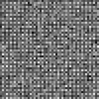
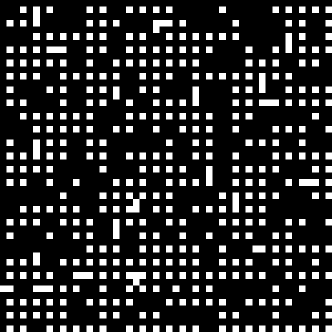
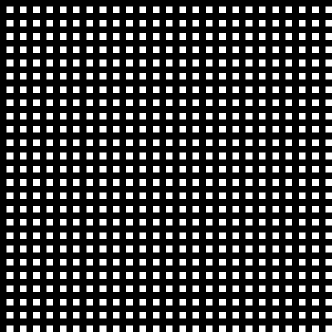
First we present an artificial example. In Fig. 5 an original grid image and its noisy version with white Gaussian noise of standard deviation are shown. The noisy image was segmented by minimizing the proposed convex functional with TV regularization (bottom left) and shearlet regularization (bottom right). As codebook we have used the exact values 0 and 1. While the first method fails to reconstruct the grid, our shearlet segmentation method works perfect. An exact reconstruction can be also obtained by applying the NL-means regularizer. However in its isotropic version the later method requires more time than the shearlet approach.

, , 300 iterations
, , 10 iterations
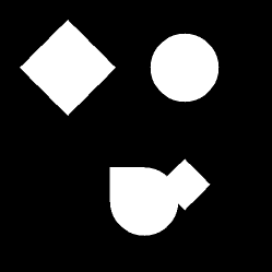
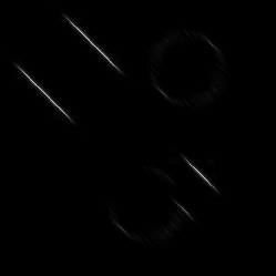
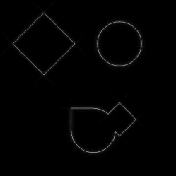
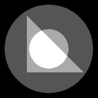
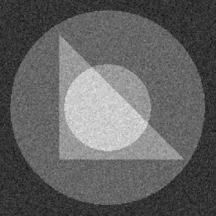
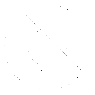
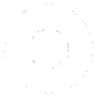
Next we want to segment the cartoon type image in Fig. 6. The top left image (Fig. 6(a)) shows the original cartoon image with four constant regions. The image was taken from [7]. In the top right image white Gaussian noise of standard deviation was added (Fig. 6(b)). The bottom row shows the difference between the segmented image and the original one. For the left image (Fig. 6(c)) the TV regularizer was used and for the right image (Fig. 6(d)) the shearlet regularizer. In both images a white pixel represents the correctly labeled pixels and the black pixels indicate false labeled pixels. Both methods have problems with correctly labeling the borders of the circles and the TV method also fails on assigning the correct labels for the diagonal border of the triangle whereas the shearlet regularizer labels all these points in the right way.
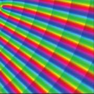
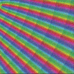
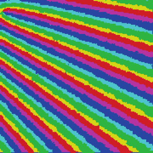
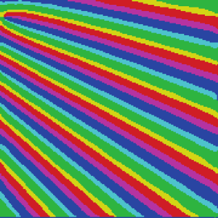
To illustrate the good performance of the shearlet regularizer for curved structures compared to the TV regularizer we provide another example using the april calender sheet of www.mathe-kalender.de, i.e., a snippet from the right bottom corner (see Fig. 7(a)). For the segmentation we added again white Gaussian noise of standard deviation in Fig. 7(b). The six different reference colors for the codebook were chose manually. In Fig. 7(c) we show the result using the TV regularizer and in Fig. 7(d) we used the shearlet regularizer. Our shearlet method preserves the stripes better than the first method. Adding more noise the results using TV become worse whereas the results using shearlets remain similar.
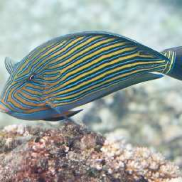
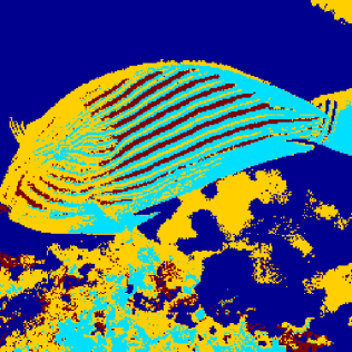
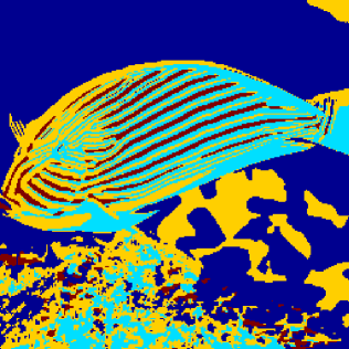
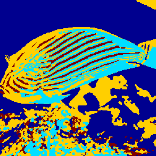
Last we want to segment the real image in Fig. 8, where 8(a) is the original RGB image of a clown-surgeon fish and in 8(b) white Gaussian noise of standard deviation was added. As codebook we use the matrix
where each row represents a color channel and each column stands for one label. The colors were chosen manually according to the different regions of the image. Compared to the segmentation model above for gray valued images only the computation of in (6) has to be slightly modified. Assuming that every pixel in the image consists of a three element vector we compute as the norm of the difference between the vectors and - in formulas:
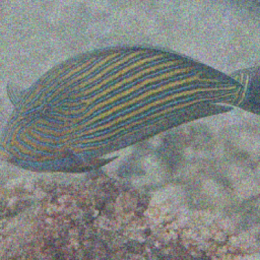
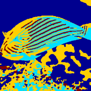
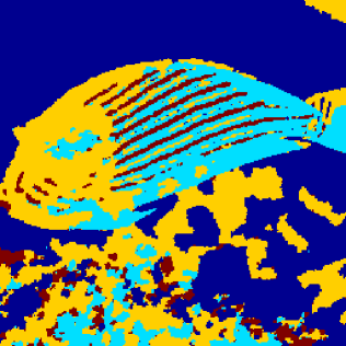
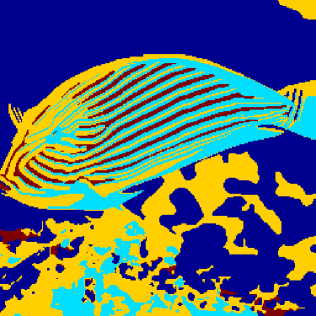
In Fig. 9 we compare the segmentation results for both images when applying different regularizers in the minimization functional.
The first row (Fig. 9(a) and 9(b)) was segmented using the TV regularizer. The second row (Fig. 9(c) and 9(d)) is obtained with the NL regularizer. The last row (Fig. 9(e) and 9(f)) shows our shearlet regularization. The parameter were chosen such that we get visually the best result. For the original image the results are rather similar with slight difficulties for the TV-model to segment the curves in the front of the fish. For the noisy image the results for the TV-based method get worse. As expected for different parameters either noise and structure is preserved or the noise vanishes in the segmentation process but we loose some structure, too. However, the TV method is the fastest one. The NL-means regularizer does a good job, but requires more computational time than our shearlet method and tends to preserve tiny structures. Our shearlet method segments this kind of curved structure very well.
, , 100 iterations
, , 100 iterations
, , 100 iterations
, , 100 iterations
, ,
30 iterations
, ,
30 iterations
In summary we have seen that shearlets can be successfully applied for the segmentation of curved textures in conjunction with a convex multi-label model and the ADMM algorithm.
References
- [1] E. Bae and X.-C. Tai. Graph cut optimization for the piecewise constant level set method applied to multiphase image segmentation. In X.-C. Tai, K. Mørken, M. Lysaker, and K.-A. Lie, editors, Scale Space and Variational Methods in Computer Vision, pages 1–13. Springer, 2009.
- [2] E. Bae, J. Yuan, and X.-C. Tai. Global minimization for continuous multiphase partitioning problems using a dual approach. International Journal of Computer Vision, 92(1):112–129, 2011.
- [3] E. Bae, J. Yuan, and X.-C. Tai. Simultaneous convex optimization of regions and region parameters in image segmentation models. In A. Bruhn, T. Pock, and X.-C. Tai, editors, Dagstuhl Reports, volume 11, pages 66–90. Schloss Dagstuhl–Leibniz-Zentrum fuer Informatik, 2011.
- [4] S. Boyd, N. Parikh, E. Chu, B. Peleato, and J. Eckstein. Distributed optimization and statistical learning via the alternating direction method of multipliers. Foundations and Trends in Machine Learning, 3(1):1–122, 2011.
- [5] Y. Boykov, O. Veksler, and R. Zabih. Fast approximate energy minimization via graph cuts. IEEE Transactions on Pattern Analysis and Machine Intelligence, 23:1222–1239, 2001.
- [6] A. Buades, B. Coll, and J.-M. Morel. A non-local algorithm for image denoising. In IEEE Computer Society Conference on Computer Vision and Pattern Recognition, volume 2, pages 60–65, 2005.
- [7] X. Cai, R. Chan, and T. Zeng. Image segmentation by convex approximation of the mumford-shah model. Preprint, The Chinese University of Hong Kong, 2012.
- [8] E. Candes, L. Demanet, D. Donoho, and L. Ying. Fast discrete curvelet transforms. Multiscale modeling and simulation, 5(3):861–899, 2006.
- [9] E. J. Candès and D. L. Donoho. Ridgelets: a key to higher-dimensional intermittency? Philosophical Transactions of the London Royal Society, 357:2495–2509, 1999.
- [10] A. Chambolle and T. Pock. A first-order primal-dual algorithm for convex problems with applications to imaging. Journal of Mathematical Imaging and Vision, 40(1):120–145, 2011.
- [11] C. Chaux, A. Jezierska, J. Pesquet, and H. Talbot. A spatial regularization approach for vector quantization. Journal of Mathematical Imaging and Vision, 41(1):23–38, 2011.
- [12] O. Christensen. An Introduction to Frames and Riesz Bases. Birkhäuser, Boston, 2003.
- [13] S. Dahlke, G. Kutyniok, P. Maass, C. Sagiv, H.-G. Stark, and G. Teschke. The uncertainty principle associated with the continuous shearlet transform. International Journal on Wavelets Multiresolution and Information Processing, 6:157–181, 2008.
- [14] S. Dahlke, G. Kutyniok, G. Steidl, and G. Teschke. Shearlet coorbit spaces and associated banach frames. Applied and Computational Harmonic Analysis, 27(2):195–214, 2009.
- [15] J. Eckstein and D. P. Bertsekas. On the Douglas-Rachford splitting method and the proximal point algorithm for maximal monotone operators. Mathematical Programming, 55:293–318, 1992.
- [16] N. El-Zehiry and L. Grady. Discrete optimization of the multiphase piecewise constant mumford-shah functional. 6819:233–246, 2011. 10.1007/978-3-642-23094-3_17.
- [17] E. Esser, X. Zhang, and T. F. Chan. A general framework for a class of first order primal-dual algorithms for convex optimization in imaging science. SIAM J. Imaging Sciences, 3(4):1015–1046, 2010.
- [18] D. Gabay. Applications of the method of multipliers to variational inequalities. In M. Fortin and R. Glowinski, editors, Augmented Lagrangian Methods: Applications to the Solution of Boundary Value Problems, chapter IX, pages 299–340. North-Holland, Amsterdam, 1983.
- [19] G. Gilboa and S. Osher. Nonlocal linear image regularization and supervised segmentation. Multiscale Modeling & Simulation, 6(2):595–630, 2007.
- [20] G. Gilboa and S. Osher. Nonlocal operators with applications to image processing. Multiscale Modeling & Simulation, 7(3):1005–1028, 2008.
- [21] T. Goldstein and S. Osher. The split Bregman method for l1-regularized problems. SIAM Journal on Imaging Sciences, 2(2):323–343, 2009.
- [22] K. Guo and D. Labate. Characterization and analysis of edges using the continuous shearlet transform. SIAM Journal on Imaging Sciences, 2(3):959–986, 2009.
- [23] K. Guo and D. Labate. The construction of smooth parseval frames of shearlets. preprint, 2011.
- [24] S. Häuser. Fast finite shearlet transform: a tutorial. Preprint University of Kaiserslautern, 2011.
- [25] Y. He, M. Y. Hussaini, J. Ma, B. Shafei, and G. Steidl. A new fuzzy c-means method with total variation regularization for segmentation of images with noisy and incomplete data. Preprint University of Kaiserslautern, 2011.
- [26] Y. M. Jung, S. H. Kang, and J. Shen. Multiphase image segmentation via modica-mortola phase transition. SIAM Journal on Applied Mathematics, 67(5):1213–1232, 2007.
- [27] S. H. Kang, B. Sandberg, and A. M. Yip. A regularized k-means and multiphase scale segmentation. Inverse Problems and Imaging, 5(2):407–429, 2011.
- [28] G. Kutyniok, K. Guo, and D. Labate. Sparse multidimensional representations using anisotropic dilation and shear operators. Wavelets und Splines (Athens, GA, 2005), G. Chen und MJ Lai, eds., Nashboro Press, Nashville, TN, pages 189–201, 2006.
- [29] G. Kutyniok and W.-Q. Lim. Image separation using wavelets and shearlets. In J.-D. Boissonnat, P. Chenin, A. Cohen, C. Gout, T. Lyche, M.-L. Mazure, and L. Schumaker, editors, Curves and Surfaces, volume 6920 of Lecture Notes in Computer Science, pages 416–430. Springer Berlin / Heidelberg, 2012. 10.1007/978-3-642-27413-8_26.
- [30] D. Labate, G. Easley, and W. Lim. Sparse directional image representations using the discrete shearlet transform. Applied and Computational Harmonic Analysis, 25(1):25–46, 2008.
- [31] R. S. Laugesen, N. Weaver, G. L. Weiss, and E. N. Wilson. A characterization of the higher dimensional groups associated with continuous wavelets. The Journal of Geometrical Analysis, 12(1):89–102, 2002.
- [32] J. Lellmann, F. Becker, and C. Schnörr. Convex optimization for multi-class image labeling with a novel family of total variation based regularizers. In International Conference on Computer Vision, 2009, IEEE, pages 646–653, October 2009.
- [33] J. Lellmann, J. Kappes, J. Yuan, F. Becker, and C. Schnörr. Convex multi-class image labeling with simplex-constrained total variation. In X.-C. Tai, K. Morken, M. Lysaker, and K.-A. Lie, editors, Scale Space and Variational Methods, volume 5567 of LNCS, volume 5567 of Lecture Notes in Computer Science, pages 150–162. Springer, 2009.
- [34] J. Lellmann and C. Schnörr. Continuous multiclass labeling approaches and algorithms. Preprint, University of Heidelberg, 2010.
- [35] J. Ma and G. Plonka. Computing with curvelets: From image processing to turbulent flows. Computing in Science & Engineering, 11(2):72–80, 2009.
- [36] J. Ma and G. Plonka. The curvelet transform. IEEE Signal Processing Magazine, 27(2):118–133, 2010.
- [37] S. Mallat. A Wavelet Tour of Signal Processing: The Sparse Way. Academic Press, San Diego, 2008.
- [38] Y. Meyer. Oscillating Patterns in Image Processing and Nonlinear Evolution Equations, volume 22. AMS, Providence, 2001.
- [39] T. Pock, A. Chambolle, D. Cremers, and H. Bischof. A convex relaxation approach for computing minimal partitions. In IEEE Conference on Computer Vision and Pattern Recognition, pages 810–817, 2009.
- [40] L. Rudin, S. Osher, and E. Fatemi. Nonlinear total variation based noise removal algorithms. Physica D, 60:259–268, 1992.
- [41] B. Sandberg, S. H. Kang, and T. F. Chan. Unsupervised multiphase segmentation: A phase balancing model. Image Processing, IEEE Transactions on, 19(1):119–130, 2010.
- [42] B. Shafei and G. Steidl. Segmentation of images with separating layers by fuzzy c-means and convex optimization. J. Visual Communication and Image Representation, (23):611–621, 2012.
- [43] M. Shahram, G. Kutyniok, and X. Zhuang. Shearlab: A rational design of a digital parabolic scaling algorithm. submitted.
- [44] G. Steidl and T. Teuber. Removing multiplicative noise by Douglas-Rachford splitting methods. Journal of Mathematical Imaging and Vision, 36:168–184, 2010.
- [45] S. Yi, D. Labate, G. R. Easley, and H. Krim. A shearlet approach to edge analysis and detection. Image Processing, IEEE Transactions on, 18(5):929–941, 2009.
- [46] J. Yuan, E. Bae, Y. Boykov, and X. Tai. A continuous max-flow approach to minimal partitions with label cost prior. In Scale Space and Variational Methods in Computer Vision, pages 279–290. Springer, 2012.
- [47] C. Zach, D. Gallup, J. Frahm, and M. Niethammer. Fast global labeling for real-time stereo using multiple plane sweeps. In O. Deussen, D. Keim, and D. Saupe, editors, Vision, modeling, and visualization. Akademische Verlagsgesellschaft, October 2008.
- [48] M. Zhu and T. F. Chan. An efficient primal-dual hybrid gradient algorithm for total vatiation image restoration. UCLA CAM Report 08-34, 2008.