INSTITUT NATIONAL DE RECHERCHE EN INFORMATIQUE ET EN AUTOMATIQUE

Wave Equation Numerical Resolution: a Comprehensive Mechanized Proof of a C Program
Sylvie Boldo — François Clément — Jean-Christophe Filliâtre — Micaela Mayero — Guillaume Melquiond — Pierre Weis N° 7826
Décembre 2011

Abstract: We formally prove correct a C program that implements a numerical scheme for the resolution of the one-dimensional acoustic wave equation. Such an implementation introduces errors at several levels: the numerical scheme introduces method errors, and floating-point computations lead to round-off errors. We annotate this C program to specify both method error and round-off error. We use Frama-C to generate theorems that guarantee the soundness of the code. We discharge these theorems using SMT solvers, Gappa, and Coq. This involves a large Coq development to prove the adequacy of the C program to the numerical scheme and to bound errors. To our knowledge, this is the first time such a numerical analysis program is fully machine-checked.

Key-words: Formal proof of numerical program , Convergence of numerical scheme , Proof of C program , Coq formal proof , Acoustic wave equation , Partial differential equation , Rounding error analysis

Résolution numérique de l’équation des ondes : une preuve mécanisée complète d’un programme C

Résumé : Nous prouvons formellement la correction d’un programme C implémentant un schéma numérique pour la résolution de l’équation des ondes acoustiques en dimension 1. Une telle implémentation introduit différents types d’erreurs : l’erreur de méthode due au schéma numérique et l’erreur d’arrondi due aux calculs en virgule flottante. Nous annotons ce programme C pour spécifier ces deux types d’erreur. Nous utilisons Frama-C pour générer les théorèmes qui garantissent la correction du code. Nous prouvons ces théorèmes à l’aide de solveurs SMT, de Gappa et de Coq. Un développement Coq important est nécessaire pour prouver l’adéquation du programme C au schéma numérique et pour borner les erreurs. À notre connaissance, c’est la première fois qu’un tel programme d’analyse numérique est complètement vérifié mécaniquement.

Mots-clés : preuve formelle d’un programme numérique, convergence d’un schéma numérique, preuve de programme C, preuve formelle en Coq, équation des ondes acoustiques, équation aux dérivées partielles, analyse d’erreur d’arrondi.

1 Introduction

Ordinary differential equations (ODE) and partial differential equations (PDE) are ubiquitous in engineering and scientific computing. They show up in nuclear simulation, weather forecast, and more generally in numerical simulation, including block diagram modelization. Since solutions to nontrivial problems are non-analytic, they must be approximated by numerical schemes over discrete grids.

Numerical analysis is a part of applied mathematics that is mainly interested in proving the convergence of these schemes [22], that is, proving that approximation quality increases as the size of discretization steps decreases. The approximation quality represents the distance between the exact continuous solution and the approximated discrete solution; this distance must tend toward zero in order for the numerical scheme to be useful.

A numerical scheme is typically proved to be convergent with pen and paper. This is a difficult, time-consuming, and error-prone task. Then the scheme is implemented as a C/C++ or Fortran program. This introduces new issues. First, we must ensure that the program correctly implements the scheme and is immune from runtime errors such as out-of-bounds accesses or overflows. Second, the program introduces round-off errors due to floating-point computations and we must prove that those errors could not lead to irrelevant results. Typical pen-and-paper proofs do not address floating-point nor runtime errors. Indeed the huge number of proof obligations, and their complexity, make the whole process almost intractable. However, with the help of mechanized program verification, such a proof becomes feasible. In the first place, because automated theorem provers can alleviate the proof burden. More importantly, because the proof is guaranteed to cover all aspects of the verification.

Our case study.

We consider the acoustic wave equation in an one-dimensional space domain. The equation describes the propagation of pressure variations (or sound waves) in a fluid medium; it also models the behavior of a vibrating string. Among the wide variety of numerical schemes to approximate the 1D acoustic wave equation, we choose the simplest one: the second order centered finite difference scheme, also known as three-point scheme. To keep it simple, we assume an homogeneous medium (the propagation velocity is constant) and we consider discretization over regular grids with constant discretization steps for time and space. Our goal is to prove the correctness of a C program implementing this scheme.

Method and tools.

We use the Jessie plug-in of Frama-C [44, 33] to perform the deductive verification of this C program. The source code is augmented with ACSL annotations [6] to describe its formal specification. When submitted to Frama-C, proof obligations are generated. Once these theorems are proved, the program is guaranteed to satisfy its specification and to be free from runtime errors. Part of the proof obligations are discharged by automated provers, e.g. Alt-Ergo [10], CVC3 [5], Gappa [25], and Z3 [28]. The more complicated ones, such as the one related to the convergence of the numerical scheme, cannot be proved automatically. These obligations were manually proved with the Coq [8, 20] interactive proof assistant. In the end, we have formally verified all the properties of the C program. To our knowledge, this is the first time this kind of verification is machine-checked. The annotated C program and the Coq sources of the formal development are available from

http://fost.saclay.inria.fr/wave_total_error.html

State of the art.

There is an abundant literature about the convergence of numerical schemes, e.g. see [56, 58]. In particular, the convergence of the three-point scheme for the wave equation is well-known and taught relatively early [7]. Unfortunately, no article goes into all the details needed for a formal proof. These mathematical “details” may have been skipped for readability, but some mandatory details may have also been omitted due to oversights.

In the fields of automatic provers and proof assistants, few works have been done for the formalization and mechanical proofs of mathematical analysis, and even fewer works for numerical analysis. The first developments on real numbers and real analysis are from the late 90’s, in systems such as ACL2 [34], Coq [45], HOL Light [36], Isabelle [32], Mizar [54], and PVS [30]. An extensive work has been done by Harrison regarding ${\mathbb{R}}^{n}$ and the dot product [37]. Constructive real analysis [35, 24, 39] and further developments in numerical analysis [49, 50] have been carried out at Nijmegen. We can also mention the formal proof of an automatic differentiation algorithm [46].

As explained by Rosinger in 1985, old methods to bound round-off errors were based on “unrealistic linearizing assumptions” [51]. Further work was done under more realistic assumptions about round-off errors [51, 52], but none of these assumptions were proved correct with respect to the numerical schemes. As Roy and Oberkampf, we believe that round-off errors should not be treated as random variables and that traditional statistical methods should not be used [53]. They propose the use of interval arithmetic or increased precision to control accuracy. Note that their example of hypersonic nozzle flow is converging so fast that round-off errors can be neglected [53]. Interval arithmetic can also take method error into account [55]. The final interval is then claimed to contain the exact solution. This is not formally proved, though. Additionally, the width of the final interval can be quite large.

There are other tools to bound round-off errors not dedicated to numerical schemes. Some successful approaches are based on abstract interpretation [23, 29]. In our case, they are of little help, since there is a complex phenomenon of error compensation during the computations. Ignoring this compensation would lead to bounds on round-off errors growing as fast as $O(2^{k})$ ($k$ being the number of time steps). That is why we had to thoroughly study the propagation of round-off errors in this numerical scheme to get tighter bounds. It also means that most of the proofs had to be done by hand to achieve this part of the formal verification.

Outline.

Section 2 presents the PDE, the numerical scheme, and their mathematical properties. Section 3 is devoted to the proofs of the convergence of the numerical scheme and the upper bound for the round-off error. Finally, Section 4 describes the formalization, i.e. the tools used, the annotated C program, and the mechanized proofs.

2 Numerical Scheme for the Wave Equation

A partial differential equation (PDE) modeling an evolution problem is an equation involving partial derivatives of an unknown function of several independent space and time variables. The uniqueness of the solution is obtained by imposing initial conditions, i.e. values of the function and some of its derivatives at initial time. The problem of the vibrating string tied down at both ends, among many other physical problems, is formulated as an initial-boundary value problem where the boundary conditions are additional constraints set on the boundary of the supposedly bounded domain [56].

This section, as well as the steps taken at Section 3.1 to conduct the convergence proof of the numerical scheme, is inspired by [7].

2.1 The Continuous Equation

The chosen PDE models the propagation of waves along an ideal vibrating elastic string that is tied down at both ends, see [1, 18], see also Figure 1. The PDE is obtained from Newton’s laws of motion [48].

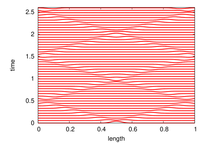
Figure 1: Space-time representation of the signal propagating along a vibrating string. Each curve represents the string at a different time step.

The gravity is neglected, so the string is supposed rectilinear when at rest. Let $x_{\rm min}$ and $x_{\rm max}$ be the abscissas of the extremities of the string. Let $\Omega=[x_{\rm min},x_{\rm max}]$ be the bounded space domain. Let $p(x,t)$ be the transverse displacement of the point of the string of abscissa $x$ at time $t$ from its equilibrium position; it is a (signed) scalar. Let $c$ be the constant propagation velocity; it is a positive number that depends on the section and density of the string. Let $s(x,t)$ be the external action on the point of abscissa $x$ at time $t$; it is a source term, such that $t=0\Rightarrow s(x,t)=0$. Finally, let $p_{0}(x)$ and $p_{1}(x)$ be the initial position and velocity of the point of abscissa $x$. We consider the initial-boundary value problem

(1) $$\forall t\geq 0,\;\forall x\in\Omega, (L(c)\,p)(x,t){\;\stackrel{{\scriptstyle\text{def}}}{{=}}\;}\frac{\partial^{2}{p}}{\partial{t}^{2}}(x,t)+A(c)\,p(x,t)=s(x,t),$$

(2) $$\forall x\in\Omega, (L_{1}\,p)(x,0){\;\stackrel{{\scriptstyle\text{def}}}{{=}}\;}\frac{\partial{p}}{\partial{t}}(x,0)=p_{1}(x),$$

(3) $$\forall x\in\Omega, (L_{0}\,p)(x,0){\;\stackrel{{\scriptstyle\text{def}}}{{=}}\;}p(x,0)=p_{0}(x),$$

(4) $$\forall t\geq 0, p(x_{\rm min},t)=p(x_{\rm max},t)=0$$

where the differential operator $A(c)$ is defined by

(5) $$A(c){\;\stackrel{{\scriptstyle\text{def}}}{{=}}\;}-c^{2}\frac{\partial^{2}{}}{\partial{x}^{2}}.$$

This simple partial derivative equation happens to possess an analytical solution given by the so-called d’Alembert’s formula [40], obtained from the method of characteristics and the image theory [38], $\forall t\geq 0$, $\forall x\in\Omega$,

(6) $$p(x,t)=\frac{1}{2}(\tilde{p}_{0}(x-ct)+\tilde{p}_{0}(x+ct))+\frac{1}{2c}\int_{x-ct}^{x+ct}\tilde{p}_{1}(y)dy+\hbox{}\frac{1}{2c}\int_{0}^{t}\left(\int_{x-c(t-\sigma)}^{x+c(t-\sigma)}\tilde{s}(y,\sigma)dy\right)d\sigma$$

where the quantities $\tilde{p}_{0}$, $\tilde{p}_{1}$, and $\tilde{s}$ are respectively the successive antisymmetric extensions in space of $p_{0}$, $p_{1}$, and $s$ defined on $\Omega$ to the entire real axis ${\mathbb{R}}$.

We have formally verified d’Alembert’s formula as a separate work [42]. But for the purpose of the current work, we just admit that under reasonable conditions on the Cauchy data $p_{0}$ and $p_{1}$ and on the source term $s$, there exists a unique solution $p$ to the initial-boundary value problem (1)–(4) for each $c>0$. Simply supposing the existence of a solution instead of exhibiting it, opens the way to scale our approach to more general cases for which there is no known analytic expression of a solution, e.g. in the case of a nonuniform propagation velocity $c$.

For such a solution $p$, it is natural to associate at each time $t$ the positive definite quadratic quantity

(7) $$E(c)(p)(t){\;\stackrel{{\scriptstyle\text{def}}}{{=}}\;}\frac{1}{2}\left\|\left(x\mapsto\frac{\partial{p}}{\partial{t}}(x,t)\right)\right\|^{2}+\frac{1}{2}\left\|(x\mapsto p(x,t))\right\|_{A(c)}^{2}$$

where $\left<q,r\right>{\;\stackrel{{\scriptstyle\text{def}}}{{=}}\;}\int_{\Omega}q(x)r(x)dx$, $\left\|q\right\|^{2}{\;\stackrel{{\scriptstyle\text{def}}}{{=}}\;}\left<q,q\right>$ and $\left\|q\right\|_{A(c)}^{2}{\;\stackrel{{\scriptstyle\text{def}}}{{=}}\;}\left<A(c)\,q,q\right>$. The first term is interpreted as the kinetic energy, and the second term as the potential energy, making $E$ the mechanical energy of the vibrating string.

2.2 The Discrete Equations

Let $i_{\rm max}$ be the positive number of intervals of the space discretization. Let the space discretization step $\Delta x$ and the discretization function $i_{\Delta x}$ be defined as

$$\Delta x{\;\stackrel{{\scriptstyle\text{def}}}{{=}}\;}\frac{x_{\rm max}-x_{\rm min}}{i_{\rm max}}\quad\mbox{and}\quad i_{\Delta x}(x){\;\stackrel{{\scriptstyle\text{def}}}{{=}}\;}\left\lfloor\frac{x-x_{\rm min}}{\Delta x}\right\rfloor.$$

Let us consider the time interval $[0,t_{\rm max}]$. Let $\Delta t\in]0,t_{\rm max}[$ be the time discretization step. We define

$$k_{\Delta t}(t){\;\stackrel{{\scriptstyle\text{def}}}{{=}}\;}\left\lfloor\frac{t}{\Delta t}\right\rfloor\quad\mbox{and}\quad k_{\rm max}{\;\stackrel{{\scriptstyle\text{def}}}{{=}}\;}k_{\Delta t}(t_{\rm max}).$$

Now, the compact domain $\Omega\times[0,t_{\rm max}]$ is approximated by the regular discrete grid defined by

(8) $$\forall k\in[0..k_{\rm max}],\,\forall i\in[0..i_{\rm max}],\quad{\bf x}_{i}^{k}{\;\stackrel{{\scriptstyle\text{def}}}{{=}}\;}(x_{i},t^{k}){\;\stackrel{{\scriptstyle\text{def}}}{{=}}\;}(x_{\rm min}+i\Delta x,k\Delta t).$$

For a function $q$ defined over $\Omega\times[0,t_{\rm max}]$ (resp. $\Omega$), the notation $q_{\rm h}$ denotes any discrete approximation of $q$ at the points of the grid, i.e. a discrete function over $[0..i_{\rm max}]\times[0..k_{\rm max}]$ (resp. $[0..i_{\rm max}]$). By extension, the notation $q_{\rm h}$ is also a shortcut to denote the matrix $(q_{i}^{k})_{0\leq i\leq i_{\rm max},0\leq k\leq k_{\rm max}}$ (resp. the vector $(q_{i})_{0\leq i\leq i_{\rm max}}$). The notation $\bar{q}_{\rm h}$ is reserved to the approximation defined on $[0..i_{\rm max}]\times[0..k_{\rm max}]$ by

$$\bar{q}_{i}^{k}{\;\stackrel{{\scriptstyle\text{def}}}{{=}}\;}q({\bf x}_{i}^{k})\quad\mbox{(resp. $\bar{q}_{i}{\;\stackrel{{\scriptstyle\text{def}}}{{=}}\;}q(x_{i})$).}$$

Figure 2: Three-point scheme: $p_{i}^{k+1}$ (at $\times$) depends on $p_{i-1}^{k}$, $p_{i}^{k}$, $p_{i+1}^{k}$, and $p_{i}^{k-1}$ (at $\bullet$).

Let $p_{0{\rm h}}$ and $p_{1{\rm h}}$ be two discrete functions over $[0..i_{\rm max}]$. Let $s_{\rm h}$ be a discrete function over $[0..i_{\rm max}]\times[0..k_{\rm max}]$. Then, the discrete function $p_{\rm h}$ over $[0..i_{\rm max}]\times[0..k_{\rm max}]$ is said to be the solution of the three-point finite difference scheme, as illustrated in Figure 2, when the following set of equations holds:

(9) $$\forall k\in[2..k_{\rm max}],\,\forall i\in[1..i_{\rm max}-1],\\ (L_{\rm h}(c)\,p_{\rm h})_{i}^{k}{\;\stackrel{{\scriptstyle\text{def}}}{{=}}\;}\frac{p_{i}^{k}-2p_{i}^{k-1}+p_{i}^{k-2}}{\Delta t^{2}}+(A_{\rm h}(c)\,(i^{\prime}\mapsto p_{i^{\prime}}^{k-1}))_{i}=s_{i}^{k-1},$$

(10) $$\forall i\in[1..i_{\rm max}-1], (L_{1{\rm h}}(c)\,p_{\rm h})_{i}{\;\stackrel{{\scriptstyle\text{def}}}{{=}}\;}\frac{p_{i}^{1}-p_{i}^{0}}{\Delta t}+\frac{\Delta t}{2}(A_{\rm h}(c)\,(i^{\prime}\mapsto p_{i^{\prime}}^{0}))_{i}=p_{1,i},$$

(11) $$\forall i\in[1..i_{\rm max}-1], (L_{0{\rm h}}\,p_{\rm h})_{i}{\;\stackrel{{\scriptstyle\text{def}}}{{=}}\;}p_{i}^{0}=p_{0,i},$$

(12) $$\forall k\in[0..k_{\rm max}], p_{0}^{k}=p_{i_{\rm max}}^{k}=0$$

where the matrix $A_{\rm h}(c)$, a discrete analog of $A(c)$, is defined for any vector $q_{\rm h}$, by

(13) $$\forall i\in[1..i_{\rm max}-1],\quad\left(A_{\rm h}(c)\,q_{\rm h}\right)_{i}{\;\stackrel{{\scriptstyle\text{def}}}{{=}}\;}-c^{2}\frac{q_{i+1}-2q_{i}+q_{i-1}}{\Delta x^{2}}.$$

A discrete analog of the energy is also defined by

(14) $$E_{\rm h}(c)(p_{\rm h})^{k+\frac{1}{2}}{\;\stackrel{{\scriptstyle\text{def}}}{{=}}\;}\frac{1}{2}\left\|\left(i\mapsto\frac{p_{i}^{k+1}-p_{i}^{k}}{\Delta t}\right)\right\|_{\Delta x}^{2}+\frac{1}{2}\left<(i\mapsto p_{i}^{k}),(i\mapsto p_{i}^{k+1})\right>_{A_{h}(c)}$$

where, for any vectors $q_{\rm h}$ and $r_{\rm h}$,

$$\begin{array}[]{lclclcl}\left<q_{\rm h},r_{\rm h}\right>_{\Delta x}&{\;\stackrel{{\scriptstyle\text{def}}}{{=}}}&\sum_{i=0}^{i_{\rm max}}q_{i}r_{i}\Delta x,&&\left\|q_{\rm h}\right\|_{\Delta x}^{2}&{\;\stackrel{{\scriptstyle\text{def}}}{{=}}}&\left<q_{\rm h},q_{\rm h}\right>_{\Delta x},\\ \left<q_{\rm h},r_{\rm h}\right>_{A_{h}(c)}&{\;\stackrel{{\scriptstyle\text{def}}}{{=}}}&\left<A_{\rm h}(c)\,q_{\rm h},r_{\rm h}\right>_{\Delta x},&&\left\|q_{\rm h}\right\|_{A_{h}(c)}^{2}&{\;\stackrel{{\scriptstyle\text{def}}}{{=}}}&\left<q_{\rm h},q_{\rm h}\right>_{A_{h}(c)}.\end{array}$$

Note that the three-point scheme is parameterized by the discrete Cauchy data $p_{0{\rm h}}$ and $p_{1{\rm h}}$, and by the discrete source term $s_{\rm h}$. Of course, when these discrete inputs are respectively approximations of the continuous functions $p_{0}$, $p_{1}$, and $s$ (e.g. when $p_{0{\rm h}}=\bar{p}_{0{\rm h}}$, $p_{1{\rm h}}=\bar{p}_{1{\rm h}}$, and $s_{\rm h}=\bar{s}_{\rm h}$), then the discrete solution $p_{\rm h}$ is an approximation of the continuous solution $p$.

2.3 Convergence

Let $\xi$ be in $]0,1[$. The CFL($\xi$) condition (for Courant-Friedrichs-Lewy, see [22]) states that the discretization steps satisfy the relation

(15) $$\frac{c\Delta t}{\Delta x}\leq 1-\xi.$$

The convergence error $e_{\rm h}$ measures the distance between the continuous and discrete solutions. It is defined by

(16) $$\forall k\in[0..k_{\rm max}],\,\forall i\in[0..i_{\rm max}],\quad e_{i}^{k}{\;\stackrel{{\scriptstyle\text{def}}}{{=}}\;}\bar{p}_{i}^{k}-p_{i}^{k}.$$

Note that when $p_{0{\rm h}}=\bar{p}_{0{\rm h}}$, then for all $i$, $e_{i}^{0}=0$. The truncation error $\varepsilon_{\rm h}$ measures at which precision the continuous solution satisfies the numerical scheme. It is defined for $k\in[2..k_{\rm max}]$ and $i\in[1..i_{\rm max}-1]$ by

(17) $$\varepsilon_{i}^{k} {\;\stackrel{{\scriptstyle\text{def}}}{{=}}\;} (L_{\rm h}(c)\,\bar{p}_{\rm h})_{i}^{k}-\bar{s}_{i}^{k-1},$$

(18) $$\varepsilon_{i}^{1} {\;\stackrel{{\scriptstyle\text{def}}}{{=}}\;} (L_{1{\rm h}}(c)\,\bar{p}_{\rm h})_{i}-\bar{p}_{1,i},$$

(19) $$\varepsilon_{i}^{0} {\;\stackrel{{\scriptstyle\text{def}}}{{=}}\;} (L_{0{\rm h}}\bar{p}_{\rm h})_{i}-\bar{p}_{0,i}.$$

Again, note that when $p_{0{\rm h}}=\bar{p}_{0{\rm h}}$ and $p_{1{\rm h}}=\bar{p}_{1{\rm h}}$, then for all $i$, $\varepsilon_{i}^{0}=0$ and $\varepsilon_{i}^{1}=e_{i}^{1}/\Delta t$. Furthermore, when there is also $s_{\rm h}=\bar{s}_{\rm h}$, then the convergence error $e_{\rm h}$ is itself solution of the same numerical scheme with inputs defined by, for all $i,k$,

$$p_{0,i}=\varepsilon_{i}^{0}=0,\quad p_{1,i}=\varepsilon_{i}^{1}=\frac{e_{i}^{1}}{\Delta t},\quad\mbox{and}\leavevmode\nobreak\ s_{i}^{k}=\varepsilon_{i}^{k+1}.$$

The numerical scheme is said to be convergent of order 2 if the convergence error tends toward zero at least as fast as $\Delta x^{2}+\Delta t^{2}$ when both discretization steps tend toward zero. More precisely, the numerical scheme is said to be convergent of order ($m$,$n$) uniformly on the interval $[0,t_{\rm max}]$ if the convergence error satisfies

(20) $$\left\|\left(i\mapsto e_{i}^{k_{\Delta t}(t)}\right)\right\|_{\Delta x}=O_{[0,t_{\rm max}]}(\Delta x^{m}+\Delta t^{n}).$$

The numerical scheme is said to be consistent with the continuous problem at order 2 if the truncation error tends toward zero at least as fast as $\Delta x^{2}+\Delta t^{2}$ when the discretization steps tend toward 0. More precisely, the numerical scheme is said to be consistent with the continuous problem at order ($m$, $n$) uniformly on interval $[0,t_{\rm max}]$ if the truncation error satisfies

(21) $$\left\|\left(i\mapsto\varepsilon_{i}^{k_{\Delta t}(t)}\right)\right\|_{\Delta x}=O_{[0,t_{\rm max}]}(\Delta x^{m}+\Delta t^{n}).$$

The numerical scheme is said to be stable if the discrete solution of the associated homogeneous problem (i.e. without any source term, $s(x,t)=0$) is bounded independently of the discretization steps. More precisely, the numerical scheme is said to be stable uniformly on interval $[0,t_{\rm max}]$ if the discrete solution of the problem without any source term satisfies

(22) $$\exists\alpha,C_{1},C_{2}>0,\,\forall t\in[0,t_{\rm max}],\,\forall\Delta x,\Delta t>0,\quad\sqrt{\Delta x^{2}+\Delta t^{2}}<\alpha\Rightarrow\\ \left\|\left(i\mapsto p_{i}^{k_{\Delta t}(t)}\right)\right\|_{\Delta x}\leq(C_{1}+C_{2}t)(\left\|p_{0{\rm h}}\right\|_{\Delta x}+\left\|p_{0{\rm h}}\right\|_{A_{h}(c)}+\left\|p_{1{\rm h}}\right\|_{\Delta x}).$$

The result to be formally proved at Section 3.1 states that if the continuous solution $p$ is regular enough on $\Omega\times[0,t_{\rm max}]$ and if the discretization steps satisfy the CFL($\xi$) condition, then the three-point scheme is convergent of order (2, 2) uniformly on interval $[0,t_{\rm max}]$.

We do not admit (nor prove) the Lax equivalence theorem which stipulates that for a wide variety of problems and numerical schemes, consistency implies the equivalence between stability and convergence. Instead, we establish that consistency and stability implies convergence in the particular case of the one-dimensional acoustic wave equation.

2.4 Program

Listing 1: The main part of the C code, without annotations.

⬇

1a1 = dt/dx*v;

a = a1*a1;

/* First initial condition and boundary conditions. */

/* Left boundary. */

6p[0][0] = 0.;

/* Time iteration -1 = space loop. */

for (i=1; i<ni; i++) {

p[i][0] = p0(i*dx);

}

11/* Right boundary. */

p[ni][0] = 0.;

/* Second initial condition (with p1=0) and boundary conditions. */

/* Left boundary. */

16p[0][1] = 0.;

/* Time iteration 0 = space loop. */

for (i=1; i<ni; i++) {

dp = p[i+1][0] - 2.*p[i][0] + p[i-1][0];

p[i][1] = p[i][0] + 0.5*a*dp;

21}

/* Right boundary. */

p[ni][1] = 0.;

/* Evolution problem and boundary conditions. */

26/* Propagation = time loop. */

for (k=1; k<nk; k++) {

/* Left boundary. */

p[0][k+1] = 0.;

/* Time iteration k = space loop. */

31 for (i=1; i<ni; i++) {

dp = p[i+1][k] - 2.*p[i][k] + p[i-1][k];

p[i][k+1] = 2.*p[i][k] - p[i][k-1] + a*dp;

}

/* Right boundary. */

36 p[ni][k+1] = 0.;

}

The main part of the C program is listed in Listing 1.

The grid steps $\Delta x$ and $\Delta t$ are respectively represented by the variables dx and dt, the grid sizes $i_{\rm max}$ and $k_{\rm max}$ by the variables ni and nk, and the propagation velocity $c$ by the variable v. The initial position $p_{0{\rm h}}$ is represented by the function p0. The initial velocity $p_{1{\rm h}}$ and the source term $s_{\rm h}$ are supposed to be zero and are not represented. The discrete solution $p_{\rm h}$ is represented by the two-dimensional array p of size $(i_{\rm max}+1)\times(k_{\rm max}+1)$. (This is a simple naive implementation, a more efficient implementation would store only two time steps.)

To assemble the stiffness matrix $A_{\rm h}(c)$, we only have to compute the square of the CFL coefficient $\frac{c\Delta t}{\Delta x}$ (lines 1–2). Then, we recognize the space loops for the initial conditions: Equation (11) on lines 6–8, and Equation (10) with $p_{1{\rm h}}=0$ on lines 14–17. The space-time loop on lines 23–28 for the evolution problem comes from Equation (9). And finally, the boundary conditions of Equation (12) are spread out on lines 9–10, 18–19, and 29–30.

3 Bounding Errors

3.1 Method Error

We first present the notions necessary to formalize and prove the method error. Then, we detail how the proof is conducted: we establish the consistency, the stability and prove that these two properties imply convergence in the case of the one-dimensional acoustic wave equation.

3.1.1 Big O, Differentiability, and Regularity

When considering a big O equality $a=O(b)$, one usually assumes that $a$ and $b$ are two expressions defined over the same domain and its interpretation as a quantified formula comes naturally. Here the situation is a bit more complicated. Consider

$$f({\bf x},{\bf\Delta x})=O(g({\bf\Delta x}))$$

when $\|{\bf\Delta x}\|$ goes to 0. If one were to assume that the equality holds for any ${\bf x}\in\mathbb{R}^{2}$, one would interpret it as

$$\forall{\bf x},\exists\alpha>0,\exists C>0,\forall{\bf\Delta x},\quad\|{\bf\Delta x}\|\leq\alpha\Rightarrow|f({\bf x},{\bf\Delta x})|\leq C\cdot|g({\bf\Delta x})|,$$

which means that constants $\alpha$ and $C$ are in fact functions of ${\bf x}$. Such an interpretation happens to be useless, since the infimum of $\alpha$ may well be zero while the supremum of $C$ may be $+\infty$.

A proper interpretation requires the introduction of a uniform big O relation with respect to the additional variable ${\bf x}$:

(23) $$\exists\alpha>0,\,\exists C>0,\,\forall{\bf x}\in\Omega_{\bf x},\,\forall{\bf\Delta x}\in\Omega_{\bf\Delta x},\hbox{}\|{\bf\Delta x}\|\leq\alpha\Rightarrow|f({\bf x},{\bf\Delta x})|\leq C\cdot|g({\bf\Delta x})|.$$

To emphasize the dependency on the two subsets $\Omega_{\bf x}$ and $\Omega_{\bf\Delta x}$, uniform big O equalities are now written

$$f({\bf x},{\bf\Delta x})=O_{\Omega_{\bf x},\Omega_{\bf\Delta x}}(g({\bf\Delta x})).$$

We now precisely define the notion of “sufficiently regular” functions in terms of the full-fledged notation for the big O. The further result on the convergence of the numerical scheme requires that the solution of the continuous equation is actually sufficiently regular. We introduce two operators that, given a real-valued function $f$ defined on the 2D plane and a point in the plane, return the values $\frac{\partial f}{\partial x}$ and $\frac{\partial f}{\partial t}$ at this point. Given these two operators, we can define the usual 2D Taylor polynomial of order $n$ of a function $f$:

$$\mathrm{TP}_{n}(f,{\bf x}){\;\stackrel{{\scriptstyle\text{def}}}{{=}}\;}(\Delta x,\Delta t)\mapsto\sum_{p=0}^{n}\frac{1}{p!}\left(\sum_{m=0}^{p}\binom{p}{m}\cdot\frac{\partial^{p}f}{\partial x^{m}\partial t^{p-m}}({\bf x})\cdot\Delta x^{m}\cdot\Delta t^{p-m}\right).$$

Let $\Omega_{\bf x}\subset{\mathbb{R}}^{2}$. We say that the previous Taylor polynomial is a uniform approximation of order $n$ of $f$ on $\Omega_{\bf x}$ when the following uniform big O equality holds:

$$f({\bf x}+{\bf\Delta x})-\mathrm{TP}_{n}(f,{\bf x})({\bf\Delta x})=O_{\Omega_{\bf x},{\mathbb{R}}^{2}}\left(\|{\bf\Delta x}\|^{n+1}\right).$$

A function $f$ is then said to be sufficiently regular of order $n$ uniformly on $\Omega_{\bf x}$ when all its Taylor polynomials of order smaller than $n$ are uniform approximations of $f$ on $\Omega_{\bf x}$.

3.1.2 Consistency

The consistency of a numerical scheme expresses that, for ${\bf\Delta x}$ small enough, the continuous solution taken at the points of the grid almost solves the numerical scheme. More precisely, we formally prove that when the continuous solution of the wave equation (1)–(4) is sufficiently regular of order 4 uniformly on $[x_{\rm min},x_{\rm max}]\times[0,t_{\rm max}]$, the numerical scheme (9)–(12) is consistent with the continuous problem at order (2, 2) uniformly on interval $[0,t_{\rm max}]$ (see definition (21) in Section 2.3). This is obtained using the properties of Taylor approximations; the proof is straightforward while involving long and complex expressions.

The key idea is to always manipulate uniform Taylor approximations that will be valid for all points of all grids when the discretization steps goes down to zero.

For instance, to take into account the initialization phase corresponding to Equation (10), we have to derive a uniform Taylor approximation of order 1 for the following continuous function (for any $v$ sufficiently regular of order 3)

$$((x,t),(\Delta x,\Delta t))\mapsto\hbox{}\frac{v(x,t+\Delta t)-v(x,t)}{\Delta t}-\frac{\Delta t}{2}c^{2}\frac{v(x+\Delta x,t)-2v(x,t)+v(x-\Delta x,t)}{\Delta x^{2}}.$$

Note that the expression of this function involves both $x+\Delta x$ and $x-\Delta x$, meaning that we need a Taylor approximation which is valid for both positive and negative growths. The proof would have been impossible if we had required $0<\Delta x$ (as a space grid step) in the definition of the Taylor approximation.

In contrast with the case of an infinite string [13], we do not need here a lower bound for $c\frac{\Delta t}{\Delta x}$.

3.1.3 Stability

The stability of a numerical scheme expresses that the growth of the discrete solution is somehow bounded in terms of the input data (here, the Cauchy data $u_{0{\rm h}}$ and $u_{1{\rm h}}$, and the source term $s_{\rm h}$). For the proof of the round-off error (see Section 3.2), we need a statement of the same form as definition (22) of Section 2.3. Therefore, we formally prove that, under the CFL$(\xi)$ condition (15), the numerical scheme (9)–(12) is stable uniformly on interval $[0,t_{\rm max}]$.

But, as we choose to prove the convergence of the numerical scheme by using an energetic technique, it is more convenient to formulate the stability in terms of the discrete energy. More precisely, we also formally prove that under the CFL$(\xi)$ condition (15), the discrete energy (14) satisfies the following overestimation,

$$\sqrt{E_{\rm h}(c)(p_{\rm h})^{k+\frac{1}{2}}}\leq\sqrt{E_{\rm h}(c)(p_{\rm h})^{\frac{1}{2}}}+\frac{\sqrt{2}}{2\sqrt{2\xi-\xi^{2}}}\cdot\Delta t\cdot\sum_{k^{\prime}=1}^{k}\left\|\left(i\mapsto s_{i}^{k^{\prime}}\right)\right\|_{\Delta x}$$

for all $t\in[0,t_{\rm max}]$ and with $k=\left\lfloor\frac{t}{\Delta t}\right\rfloor-1$.

The evolution of the discrete energy between two consecutive time steps is shown to be proportional to the source term. In particular, the energy is constant when the source is inactive. Then, we obtain the following underestimation of the discrete energy,

$$\forall k,\quad\frac{1}{2}\left(1-\left(c\frac{\Delta t}{\Delta x}\right)^{2}\right)\left\|\left(i\mapsto\frac{p_{i}^{k+1}-p_{i}^{k}}{\Delta t}\right)\right\|_{\Delta x}\leq{E_{\rm h}(c)(p_{\rm h})^{k+\frac{1}{2}}}.$$

Therefore, the non-negativity of the discrete energy is directly related to the CFL$(\xi)$ condition.

Note that this stability result is valid for any input data $p_{0{\rm h}}$, $p_{1{\rm h}}$, and $s_{\rm h}$.

3.1.4 Convergence

The convergence of a numerical scheme expresses the fact that the discrete solution gets closer to the continuous solution as the discretization steps go down to zero. More precisely, we formally prove that when the continuous solution of the wave equation (1)–(4) is sufficiently regular of order 4 uniformly on $[x_{\rm min},x_{\rm max}]\times[0,t_{\rm max}]$, and under the CFL$(\xi)$ condition (15), the numerical scheme (9)–(12) is convergent of order (2, 2) uniformly on interval $[0,t_{\rm max}]$ (see definition (20) in Section 2.3).

Firstly, we prove that the convergence error $e_{\rm h}$ is itself the discrete solution of a numerical scheme of the same form but with different input data. In particular, the source term (on the right-hand side) is here the truncation error $\varepsilon_{\rm h}$ associated with the initial numerical scheme for $p_{\rm h}$. Then, the previous stability result holds, and we have an overestimation of the square root of the discrete energy associated with the convergence error $E_{\rm h}(c)(e_{\rm h})$ that involves a sum of the corresponding source terms, i.e. the truncation error. Finally, the consistency result also makes this sum a big O of $\Delta x^{2}+\Delta t^{2}$, and a few more technical steps conclude the proof.

3.2 Round-off Error

As each operation is done with IEEE-754 floating-point numbers [47], round-off errors will occur and may endanger the accuracy of the final results. On this program, naive forward error analysis gives an error bound that is proportional to $2^{k}2^{-53}$ for the computation of a $p_{i}^{k}$. If this bound was sensible, it would cause the numerical scheme to compute only noise after a few steps. Fortunately, round-off error actually compensate themselves. To take into account the compensations and hence prove a usable error bound, we need a precise statement of the round-off error [12] to exhibit the cancellations made by the numerical scheme.

3.2.1 Local Round-off Errors

Let $\delta_{i}^{k}$ be the (signed) floating-point error made in the two lines computing $p_{i}^{k}$ (lines 26–27 in Listing 1). Floating-point values as computed by the program will be underlined: $\underline{a}$, $\underline{p}_{i}^{k}$ to distinguish them from the discrete values of previous sections. They match the expressions a and p[i][k] in the annotations, while $a$ and $p_{i}^{k}$ can be represented in the annotations by $\backslash$exact(a) and $\backslash$exact(p[i][k]), as described in Section 4.1.4.

The $\delta_{i}^{k}$ are defined as follow:

$$\delta_{i}^{k+1}=\underline{p}_{i}^{k+1}-(2\underline{p}_{i}^{k}-\underline{p}_{i}^{k-1}+a\times(\underline{p}_{i+1}^{k}-2\underline{p}_{i}^{k}+\underline{p}_{i-1}^{k})).$$

Note that the program explained in Section 2.4 gives us that

$$\underline{p}_{i}^{k+1}=\mbox{fl}\left(2\underline{p}_{i}^{k}-\underline{p}_{i}^{k-1}+\underline{a}\times(\underline{p}_{i+1}^{k}-2\underline{p}_{i}^{k}+\underline{p}_{i-1}^{k})\right)$$

where $\mbox{fl}(\cdot)$ means that all the arithmetic operations that appear between the parentheses are actually performed by floating-point arithmetic, hence a bit off.

In order to get a bound on $\delta_{i}^{k}$, we need to have the range of $\underline{p}_{i}^{k}$. For this bound to be usable in our correctness proof, we need the range to be $[-2,2]$. We have proved this fact by using the bounds on the method error and the round-off error of all the $\underline{p}^{k}$ and $\underline{p}^{k-1}$.

To prove the bound on $\delta_{i}^{k}$, we perform forward error analysis and then use interval arithmetic to bound each intermediate error. We prove that, for all $i$ and $k$, we have $|\delta_{i}^{k}|\leq 78\times 2^{-52}$ for a reasonable error bound for $a$, that is to say $|\underline{a}-a|\leq 2^{-49}$.

3.2.2 Convolution of Round-off Errors

Note that the global floating-point error $\Delta_{i}^{k}=\underline{p}_{i}^{k}-p_{i}^{k}$ depends not only on $\delta_{i}^{k}$, but also on all the $\delta_{i+j}^{k-l}$ for $0<l\leq k$ and $-l\leq j\leq l$. Indeed round-off errors propagate along floating-point computations. Their contributions to $\Delta_{i}^{k}$, which are independent and linear (due to the structure of the numerical scheme), can be computed by performing a convolution with a function $\lambda:(\mathbb{Z}\times\mathbb{Z})\rightarrow{\mathbb{R}}$. This function $\lambda$ represents the results of the numerical scheme when fed with a single unit value:

$$\begin{array}[]{c}\lambda_{0}^{0}=1\qquad\forall i\neq 0,\ \lambda_{i}^{0}=0\\[5.0pt] \lambda_{-1}^{1}=\lambda_{1}^{1}=a\qquad\lambda_{0}^{1}=2(1-a)\qquad\forall i\not\in\{-1,0,1\},\ \lambda_{i}^{1}=0\\[5.0pt] \lambda_{i}^{k}=a\times(\lambda_{i-1}^{k-1}+\lambda_{i+1}^{k-1})+2(1-a)\times\lambda_{i}^{k-1}-\lambda_{i}^{k-2}\end{array}$$

Theorem 1.

$$\Delta_{i}^{k}=\underline{p}_{i}^{k}-p_{i}^{k}=\sum_{l=0}^{k}\sum_{j=-l}^{l}\lambda_{j}^{l}\ \delta_{i+j}^{k-l}.$$

Details of the proof can be found in [12], but this point of view using convolution is new. The proof mainly amounts to performing numerous tedious transformations of summations until both sides are proved equal.

The previous proof assumes that the double summation is correct for all $(i^{\prime},k^{\prime})$ such that $k^{\prime}<k$. This would be correct if there was an unbounded set of $i$ where $p_{i}^{k}$ is computed. This is no longer the case for a finite string. Indeed, at the ends of the range ($i=0$ or $i_{\rm max}$), $p_{i}^{k}$ and $\underline{p}_{i}^{k}$ are equal to $0$, so $\Delta_{i}^{k}$ has to be $0$ too.

The solution is to define the successive antisymmetric extension in space (as is done for d’Alembert’s formula in Section 2.1) and to use it instead of $\delta$. This ensures that both $\Delta_{0}^{k}$ and $\Delta_{i_{\rm max}}^{k}$ are equal to $0$. It does not have any consequence on the values of $\Delta_{i}^{k}$ for $0<i<i_{\rm max}$.

3.2.3 Bound on the Global Round-off Error

The analytic expression of $\Delta_{i}^{k}$ can be used to obtain a bound on the round-off error. We will need two lemmas for this purpose.

Lemma 1.

$\displaystyle\sum_{i=-\infty}^{+\infty}\lambda_{i}^{k}=k+1.$

Proof.

We have

$$\sum_{i=-\infty}^{+\infty}\!\!\!\lambda_{i}^{k+1}=2\check{a}\sum_{i=-\infty}^{+\infty}\!\!\!\lambda_{i}^{k}+2(1-\check{a})\sum_{i=-\infty}^{+\infty}\!\!\!\lambda_{i}^{k}-\sum_{i=-\infty}^{+\infty}\!\!\!\lambda_{i}^{k-1}=2\sum_{i=-\infty}^{+\infty}\!\!\!\lambda_{i}^{k}-\sum_{i=-\infty}^{+\infty}\!\!\!\lambda_{i}^{k-1}.$$

The sum by line verifies a simple linear recurrence. As $\sum\lambda_{i}^{0}=1$ and $\sum\lambda_{i}^{1}=2$, we have $\sum\lambda_{i}^{k}=k+1$. ∎

Lemma 2.

$\lambda_{i}^{k}\geq 0$.

Proof.

The demonstration was found out by M. Kauers and V. Pillwein.

If we denote by $P$ the Jacobi polynomial, we have

$$\lambda_{n}^{j}=\sum_{k=j}^{n}\binom{2k}{j+k}\binom{n+k+1}{2k+1}(-1)^{j+k}a^{k}=a^{j}\sum_{k=0}^{n-j}P_{k}^{(2j,0)}(1-2a)$$

Now the conjecture follows directly from the inequality of Askey and Gasper [3], which asserts that $\sum_{k=0}^{n}P_{k}^{(r,0)}(x)>0$ for $r>-1$ and $-1<x\leq 1$ (see Theorem 7.4.2 in The Red Book [2]). ∎

Theorem 2.

$$\left|\Delta_{i}^{k}\right|=\left|\underline{p}_{i}^{k}-p_{i}^{k}\right|\leq 78\times 2^{-53}\times(k+1)\times(k+2).$$

Proof.

According to Theorem 1, $\Delta_{i}^{k}$ is equal to $\sum_{l=0}^{k}\sum_{j=-l}^{l}\lambda_{j}^{l}\ \delta_{i+j}^{k-l}$. We know that for all $j$ and $l$, $|\delta_{j}^{l}|\leq 78\times 2^{-52}$ and that $\sum\lambda_{i}^{l}=l+1$. Since the $\lambda_{i}^{k}$ are nonnegative, the error is easily bounded by $78\times 2^{-52}\times\sum_{l=0}^{k}(l+1)$. ∎

3.3 Total Error

Let $\cal E_{\rm h}$ be the total error. It is the sum of the method error (or convergence error) $e_{\rm h}$ of Sections 2.3 and 3.1.4, and of the round-off error $\Delta_{h}$ of Section 3.2.

From Theorem 2, we can estimate the following upper bound for the spatial norm of the round-off error when $\Delta x\leq 1$ and $\Delta t\leq t_{\rm max}/2$: for all $t\in[0,t_{\rm max}]$,

$$\left\|\left(i\mapsto\Delta_{i}^{k_{\Delta t}(t)}\right)\right\|_{\Delta x} = \sqrt{\sum_{i=0}^{i_{\rm max}}\left(\Delta_{i}^{k_{\Delta t}(t)}\right)^{2}\Delta x}$$

$$\leq \sqrt{(i_{\rm max}+1)\Delta x}\times 78\times 2^{-53}\times\left(\frac{t_{\rm max}}{\Delta t}+1\right)\times\left(\frac{t_{\rm max}}{\Delta t}+2\right)$$

$$\leq \sqrt{x_{\rm max}-x_{\rm min}+1}\times 78\times 2^{-53}\times 3\times\frac{t_{\rm max}^{2}}{\Delta t^{2}}.$$

Thus, from the triangular inequality for the spatial norm, we obtain the following estimation of the total error:

$$\forall t\in[0,t_{\rm max}],\;\forall{\bf\Delta x},\quad\|{\bf\Delta x}\|\leq\min(\alpha_{e},\alpha_{\Delta})\Rightarrow\hbox{}\left\|\left(i\mapsto{\cal E}_{i}^{k_{\Delta t}(t)}\right)\right\|_{\Delta x}\leq C_{e}(\Delta x^{2}+\Delta t^{2})+\frac{C_{\Delta}}{\Delta t^{2}}$$

where the convergence constants $\alpha_{e}$ and $C_{e}$ were extracted from the Coq proof (see Section 3.1.4) and are given in terms of the constants for the Taylor approximation of the exact solution at degree 3 ($\alpha_{3}$ and $C_{3}$), and at degree 4 ($\alpha_{4}$ and $C_{4}$) by

$$\alpha_{e} = \min(1,t_{\rm max},\alpha_{3},\alpha_{4}),$$

$$C_{e} = 2\mu t_{\rm max}\sqrt{x_{\rm max}-x_{\rm min}}\left(\frac{C^{\prime}}{\sqrt{2}}+\mu(t_{\rm max}+1)C^{\prime\prime}\right)$$

with $\mu=\frac{\sqrt{2}}{\sqrt{2\xi-\xi^{2}}}$, $C^{\prime}=\max(1,C_{3}+c^{2}C_{4}+1)$, and $C^{\prime\prime}=\max(C^{\prime},2(1+c^{2})C_{4})$, and where the round-off constants $\alpha_{\Delta}$ and $C_{\Delta}$, as explained above, are given by

$$\alpha_{\Delta} = \min(1,t_{\rm max}/2),$$

$$C_{\Delta} = 234\times 2^{-53}\times t_{\rm max}^{2}\sqrt{x_{\rm max}-x_{\rm min}+1}.$$

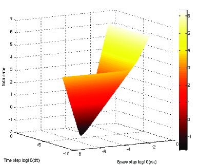
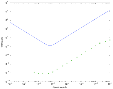
Figure 3: Upper bound for the total error in log-scale. Left: for $\Delta x$ and $\Delta t$ satisfying the CFL condition. The lighter area (in yellow) represents the higher values above $10^{4}$, whereas the darker area represents the lower values below $10^{-1}$. Right: for an optimal CFL condition with $\Delta t=\frac{1-\xi}{c}\Delta x$. The green crosses represent the effective total error computed by the C program for a few values of the space step.

To give an idea of the relative importance of both errors, we consider the academic case where the space domain is the interval $[0,1]$, the velocity of waves is $c=1$, and there is no initial velocity ($u_{1}(x)=0$) nor source term ($s(x,t)=0$). We suppose that the initial position is given by $u_{0}(x)=\chi(2(x-x_{0})/l)$ where $x_{0}=0.5$, $l=0.25$, and $\chi$ is the $C^{4}$ function defined on $[-1,1]$ by $\chi(z)=(\cos(\frac{\pi}{2}z))^{5}$, and with null continuation on the real axis. For this function, we may take $\alpha_{3}=\alpha_{4}=\sqrt{2}/2$, $C_{3}=5120\sqrt{2}$, and $C_{4}=409600/3$. The corresponding solution presents two hump-shaped signals that propagate in each direction along the string, see Figure 1.

The upper bound on the total error is represented in Figure 3. Note that everything is in logarithmic scale. Of course, decreasing the size of the grid step decreases the method error, but in the same time, it increases the round-off error. Hence, the existence of a minimum for the upper bound on the total error (about 0.02 in our test case), corresponding to optimal grid step sizes. Fortunately, the effective total error usually happens to be much smaller than this upper bound (by about a factor of $10^{6}$ in our example).

Even if the effective total error on this example is off by several orders of magnitude with respect to the theoretical bound, this experiment is still reassuring. First, the left side of Figure 3 shows that the optimal choice (the darker part) for choosing $\Delta x$ and $\Delta t$ is reached near the limit of the CFL condition. This property matches common knowledge from numerical analysis. Second, the right side shows that both the effective error and the theoretical error have the same asymptotic behavior. So the properties we have verified in this work are not intrinsically easier than the best theorems one could state. It is just that the constants of the formulas extracted from the proofs (which we did not tune for this specific purpose) are not optimal for this example.

4 Mechanization of Proofs

In Sections 3.1 and 3.2, we have mostly described the method and round-off errors introduced when solving the wave equation problem with the given numerical scheme. We do not yet know whether this formalization actually matches the program described in Section 2.4 and fully given in Appendix A. In addition, the program might contain programming errors like out-of-bound accesses, which would possibly be left unattended while comparing the program and its formalization.

To fully verify the program, our process is as follows. First, we annotated the C program with comments specifying its behavioral properties, that is, what the program is supposed to compute. Second, we let Frama-C/Why generate proof obligations that state that the program matches its specification and that its execution is safe. Third, we used automated provers and Coq to prove all of these obligations.

Section 4.1 presents all the tools we have used for verifying the C program. Then Section 4.2 explains how the program was annotated. Finally, Section 4.3 shows how we proved all the obligations, either automatically or with a proof assistant.

4.1 Tools

Several software packages are used in this work. The formal proof of the method error has been made in Coq. The formal proof of the round-off error has been made in Coq, and using the Gappa tactic. The certification of the C program has used Frama-C (with the Jessie plug-in), and to prove the produced goals, we used Gappa, SMT provers, and the preceding Coq proofs. This section is devoted to present these tools and necessary libraries.

4.1.1 Coq

Coq is a formal system that provides an expressive language to write mathematical definitions, executable algorithms, and theorems, together with an interactive environment for proving them [8]. Coq’s formal language is based on the Calculus of Inductive Constructions [21] that combines both a higher-order logic and a richly-typed functional programming language. Coq allows to define functions or predicates, that can be evaluated efficiently, to state mathematical theorems and software specifications, and to interactively develop formal proofs of these theorems. These proofs are machine-checked by a relatively small kernel, and certified programs can be extracted from them to external programming languages like Objective Caml, Haskell, or Scheme [43].

As a proof development system, Coq provides interactive proof methods, decision and semi-decision algorithms, and a tactic language for letting the user define its own proof methods. Connection with external computer algebra system or theorem provers is also available.

The Coq library is structured into two parts: the initial library, which contains elementary logical notions and data-types, and the standard library, a general-purpose library containing various developments and axiomatizations about sets, lists, sorting, arithmetic, real numbers, etc.

In this work, we mainly use the Reals standard library [45], that is a classical axiomatization of an Archimedean ordered complete field. We chose Reals to make our numerical proofs because we do not need an intuitionistic formalization.

For floating-point numbers, we use a large Coq library initially developed in [26] and extended with various results afterwards [11]. It is a high-level formalization of IEEE-754 with gradual underflow. This is expressed by a formalization where floating-point numbers are pairs $(n,e)$ associated with real values $n\times\beta^{e}$. The requirements for a number to be in the format $(e_{\min},\beta^{p})$ are

$$|n|<\beta^{p}\quad\mbox{and}\quad e_{\min}\leq e.$$

This formalization is convenient for human interactive proofs as testified by the numerous proofs using it. The huge number of lemmas available in the library (about 1400) makes it suitable for a large range of applications. This library has since then been superseded by the Flocq library [16], but it was not yet available at the time we proved the floating-point results of this work.

4.1.2 Frama-C, Jessie, Why, and the SMT Solvers

We use the Frama-C platform to perform formal verification of C programs at the source-code level. Frama-C is an extensible framework that combines static analyzers for C programs, written as plug-ins, within a single tool. In this work, we use the Jessie plug-in for deductive verification. C programs are annotated with behavioral contracts written using the ANSI C Specification Language (ACSL for short) [6]. The Jessie plug-in translates them to the Jessie language [44], which is part of the Why verification platform [31]. This part of the process is responsible for translating the semantics of C into a set of Why logical definitions (to model C types, memory heap, etc.) and Why programs (to model C programs). Finally, the Why platform computes verification conditions from these programs, using traditional techniques of weakest preconditions, and emits them to a wide set of existing theorem provers, ranging from interactive proof assistants to automated theorem provers. In this work, we use the Coq proof assistant (Section 4.1.1), SMT solvers Alt-Ergo [19], CVC3 [5] and Z3 [28], and the automated theorem prover Gappa (Section 4.1.3). Details about automated and interactive proofs can be found in Section 4.3. The dataflow from C source code to theorem provers can be depicted as follows:

More precisely, to run the tools on a C program, we use a graphical interface called gWhy. A screenshot is in Appendix B. In this interface, we may call one prover on one or on many goals. We then get a graphical view of how many goals are proved and by which prover.

In ACSL, annotations are using first-order logic. Following the programming by contract approach, the specifications involve preconditions, postconditions, and loop invariants. Contrary to other approaches focusing on run-time assertion checking, ACSL specifications do not refer to C values and functions, even if pure, but refer instead to purely logical symbols. In the following contract for a function computing the square of an integer x

⬇

//@ ensures \result == x * x;

int square(int x);

the postcondition, introduced with ensures, refers to the return value $\backslash$result and argument x. Both are denoting mathematical integer values, for the corresponding C values of type int. In particular, x $*$ x cannot overflow. Of course, one could give function square a more involved specification that handles overflows, e.g. with a precondition requiring x to be small enough. Simply speaking, we can say that C integers are reflected within specifications as mathematical integers, in an obvious way. The translation of floating-point numbers is more subtle and explained in Section 4.1.4.

4.1.3 Gappa

The Gappa tool adapts the interval-arithmetic paradigm to the proof of properties that occur when verifying numerical applications [25]. The inputs are logical formulas quantified over real numbers whose atoms are usually enclosures of arithmetic expressions inside numeric intervals. Gappa answers whether it succeeded in verifying it. In order to support program verification, one can use rounding functions inside expressions. These unary operators take a real number and return the closest real number in a given direction that is representable in a given binary floating-point format. For instance, assuming that operator $\circ$ rounds to the nearest binary64 floating-point number, the following formula states that the relative error of the floating-point addition is bounded:

$$\forall x,y\in{\mathbb{R}},\leavevmode\nobreak\ \exists\varepsilon\in{\mathbb{R}},\leavevmode\nobreak\ |\varepsilon|\leq 2^{-53}\land\circ(\circ(x)+\circ(y))=(\circ(x)+\circ(y))\times(1+\varepsilon).$$

Converting straight-line numerical programs to Gappa logical formulas is easy and the user can provide additional hints if the tool were to fail to verify a property. The tool is specially designed to handle codes that are performing convoluted manipulations. For instance, it has been successfully used to verify a state-of-the-art library of correctly-rounded elementary functions [27]. In the current work, Gappa has been used to check much simpler properties. (In particular, no user hint was needed to discharge a proof automatically.) But the length of their proofs would discourage even the most dedicated users if they were to be manually handled. One of the properties is the round-off error of a local evaluation of the numerical scheme (Section 3.2.1). Other properties mainly deal with proving that no exceptional behavior occurs while executing the program: due to the initial values, all the computed values are sufficiently small to never cause overflow.

The verification of some formulas requires reasonings that are so long and intricate [27], that it might cast some doubts on whether an automatic tool actually succeeded in proving them. This is especially true when the tool ends up proving a property stronger than what the user expected. That is why Gappa also generates a formal certificate that can be mechanically checked by a proof assistant. This feature has served as the basis for a Coq tactic for automatically solving goals related to floating-point and real arithmetic [15]. The tactic reads the current Coq goal, generates a Gappa goal, executes Gappa on it, recovers the certificate, and converts it to a complete proof term that Coq matches against the current goal. At this point, whether Gappa is correct or not no longer matters: the original Coq goal is formally proved by a complete Coq proof.

This tactic has been used whenever a verification condition would have been directly proved by Gappa, if not for some confusing notations or encodings of matrix elements. We just had to apply a few basic Coq tactics to put the goal into the proper form and then call the Gappa tactic to discharge it automatically.

4.1.4 Floating-Point Formalizations

A natural question is the link between the various representations of floating-point numbers. We assume that the execution environment (mostly the processor) complies with the IEEE-754 standard [47], which defines formats, rounding modes, and operations. The C program we consider is compiled in an assembly code that will directly use these formats and operations. We also assume that the compiler optimizations preserve the visible semantics of floating-operations from the original code, e.g. no use of the extended registers. Such optimizations could have been taken into account though, but at a cost [17].

When verifying the C program, the floating-point operations are translated by Frama-C/Jessie/Why following some previous work by two of the authors [14]. A floating-point number $f$ is modeled in the logic as a triple of real numbers $(r,e,m)$. Value $r$ simply stands for the real number that is immediately represented by $f$; value $e$ stands for the exact value of $f$, as obtained if no rounding errors had occurred; finally, value $m$ stands for the model of $f$, which is a placeholder for the value intended to be computed and filled by the user. The two latter values have no existence in the program, but are useful for the specification and the verification. In particular, they help state assertions about the rounding or the model error of a program. In ACSL, the three components of the model of a floating-point number f can be referred to using f, $\backslash$exact(f), and $\backslash$model(f), respectively. $\backslash$round_error(f) is a macro for the rounding error, that is, $\backslash$abs(f - $\backslash$exact(f)).

For instance, the following excerpt from our C program specifies the error on the content of the dx variable, which represents the grid step $\Delta x$ (see Section 2).

⬇

dx = 1./ni;

/*@ assert

@ dx > 0. && dx <= 0.5 &&

@ \abs(\exact(dx) - dx) / dx <= 0x1.p-53;

@ */

Note that 0x1.p-53 is a valid ACSL (and C too) literal meaning $2^{-53}$.

Proof obligations are extracted from the annotated C program by computing weakest preconditions and then translated to automated and interactive provers. For SMT provers, the three fields $r$, $e$, and $m$, of floating-point numbers are expressed as real numbers and operations on floating-point numbers are uninterpreted relations axiomatized with basic properties such as bounds on the rounding error or monotonicity. For Gappa too, the fields are seen as real numbers. The tool, however, knows about floating-point arithmetic and its relation to real arithmetic. So floating-point operations are translated to the corresponding symbols from Gappa.

For Coq, we use the formalization described in Section 4.1.1 with a limited precision and gradual underflow (so that subnormal numbers are correctly translated). It is based on the real numbers of the standard library, which are also used for the translation of the exact and the model parts of the floating-point number.

While the IEEE-754 standard defines infinities and Not-a-Number as floating-point values, our translation does not take them into account. This does not compromise the correctness of the translation though, as each operation has a precondition that raises a proof obligation to guarantee that no exceptional events occur, such as overflow or division by zero, and therefore no infinities nor Not-a-Number are produced by the program.

To summarize, there is one assumption about the actual arithmetic being executed (IEEE-754 compliant and no overly aggressive optimizations from the compiler) and three formalizations of floating-point arithmetic used to verify the program: one used by Jessie/Why and then sent to the SMT solvers, one used by Gappa, and one used by Coq. The combination of these three different formalizations does not introduce any inconsistency. Indeed, we have formally proved in Coq that Gappa’s and Coq’s formalizations are equivalent for floating-point formats with limited precision and gradual underflow, that is, IEEE-754 formats. We have also formally proved that the Jessie/Why specifications and the properties for SMT provers are compatible with these formalizations, including the absence of special values (infinity or Not-a-Number) and the possibility to disregard the upper bound on reals representing floating-point numbers.

In fact, there is a fourth formalization of floating-point arithmetic involved, which is the one used internally by the interval computations of Gappa for proving results about real-valued expressions. It is not equivalent to the previous ones, since it is a multi-precision arithmetic, but it has no influence whatsoever on the formalization that Gappa uses for modeling floating-point properties.

4.2 Program Annotations

The full annotations are given in Appendix A. We give here hints about how to specify this program.

There are two axiomatics. The first one corresponds to the mathematics: the exact solution of the wave equation and its properties. It defines the needed values (the exact solution $p$, and its initialization $p_{0}$). We here assume that $s$ and $p_{1}$ are zero functions. It also defines the derivatives of $p$ ($psol_{1}$, first derivative for the first variable of $p$, and $psol_{11}$, second derivative for the first variable, and $psol_{2}$ and $psol_{22}$ for the second variable) as functions such that their value is the limit of $\frac{p(x+\Delta x)-p(x)}{\Delta x}$ when $\Delta x\rightarrow 0$. As the ACSL annotations are only first order, these definitions are quite cumbersome: each derivative needs 5 lines to be defined.

We also put as axioms the fact that the solution has the expected properties (1–4). The last property needed on the exact solution is its regularity. We require it to be near its Taylor approximations of degrees 3 and 4 on the whole interval $[x_{\rm min},x_{\rm max}]$. For instance, the following annotation states the property for degree 3.

⬇

/*@ axiom psol_suff_regular_3:

@ 0 < alpha_3 && 0 < C_3 &&

@ \forall real x; \forall real t; \forall real dx; \forall real dt;

@ 0 <= x <= 1 ==> \sqrt(dx * dx + dt * dt) <= alpha_3 ==>

@ \abs(psol(x + dx, t + dt) - psol_Taylor_3(x, t, dx, dt)) <=

@ C_3 * \abs(\pow(\sqrt(dx * dx + dt * dt), 3));

@*/

The second axiomatic corresponds to the properties and loop invariant needed by the program. For example, we require the matrix to be separated: it means that a line of the matrix should not mix with another line (or a modification could alter another point of the matrix). We also state the existence of the loop invariant analytic_error that is needed for applying the results of Section 3.2.

The initializations functions are specified, but not stated. This corresponds firstly to the function array2d_alloc that initializes the matrix and p_zero that produces an approximation of the $p_{0}$ function. Our program verification is modular: our proofs are generic with respect to $p_{0}$ and its implementation.

The preconditions of the main functions are the following ones:

• $i_{\rm max}$ and $k_{\rm max}$ must be greater than one, but small enough so that $i_{\rm max}+1$ and $k_{\rm max}+1$ do not overflow;

• the grid sizes ${\bf\Delta x}$ must fulfill some mathematical conditions that are required for the convergence of the scheme;

• the floating-point values computed for the grid sizes must be near their mathematical values;

• to prevent exceptional behavior in the computation of $a$, the time discretization step must be greater than $2^{-1000}$ and $\frac{c\Delta t}{\Delta x}$ must be greater than $2^{-500}$.

There are two postconditions, corresponding to the method and round-off errors. See Sections 3.1 and 3.2 for more details.

4.3 Automation and Manual Proofs

This section is devoted to formal specifications and proofs corresponding to the bounds proved in Section 3. We give some key points of the automated proofs.

Big O.

In section 3.1.1, we present two interpretations of the big O notation. Usual mathematical pen-and-paper proofs switch from one interpretation to the other depending on which one is the most adapted, without noticing that they may not be equivalent. The formal development was helpful in bringing into light the erroneous reasoning hidden by the usage of big O notations. We introduced the notion of uniform big O in [13] in the context of an infinite string. In the present paper, we consider the case of the finite string, hence for compactness reasons, both notions are in fact equivalent. However, we still use the more general uniform big O notion to share most of the proof developments between the finite and the infinite cases. Regarding automation, a decision procedure has been developed in [4]; unfortunately, those results were not applicable since we needed a more powerful big O.

Differential operators.

As long as we were studying only the method error, we did not have to define the differential operators nor assume anything about them [13]. Their only properties appeared through their usage: function $p$ is a solution of the partial differential equation and it is sufficiently regular. This is no longer possible for the annotated C program. Indeed, due to the underlying logic, the annotations have to define $p$ as a solution of the PDE by using first-order formulas stating differentiability, instead of second-order formulas involving differential operators. Since the formalization of Taylor approximations has been left unchanged, the natural way to relate the C annotations with the Coq development is therefore to define the operators as actual differential operators. Note that this has forced us to introduce a small axiom. Indeed, our definition of Taylor approximation depends on differential operators that are total functions, while Coq’s standard library defines only partial operators. So we have assumed the existence of some total operators that are equal to the partial ones whenever applied to differentiable functions. The axiom states absolutely nothing about the result of these operators for nondifferentiable functions, so no inconsistencies are introduced this way. This is just a specific instance of Hilbert $\varepsilon$ operator [57], which does not make the logic inconsistent [41].

Method error.

The Coq proof of the method error is about 5000-line long. About half of it is dedicated to the wave equation and the other half is re-usable (definition and properties of the dot product, the big O, Taylor expansions…). We formally proved without any axiom that the numerical scheme is convergent of order 2, which is the known mathematical result. An interesting aspect of the formal proof in Coq is that we were able to extract the constants $\alpha$ and $C$ appearing in the big O for the convergence result in order to obtain their precise values. The recursive extraction was fully automatic after making explicit some inlining. The mathematical expressions are given in Section 3.3.

Round-off errors.

Except for Lemma 2, all the proofs described in section 3.2 have been done and machined-checked using Coq. In particular, the proof of the bound on $\delta_{i}^{k}$ was done automatically by calling Gappa from Coq. Lemma 2 is a technical detail compared to the rest of our work, that is not worth the immense Coq development it would require: keen results on integrals but also definitions and results about the Legendre, Laguerre, Chebychev, and Jacobi polynomials.

The program proof.

Given the program code, the Why tool generates 149 verification conditions that have to be proved. While possible, proving all of them in Coq would be rather tedious. Moreover, it would lead to a rather fragile construct: any later modification to the code, however small it is, would cause different proof obligations to be generated, which would then require additional human interaction to adapt the Coq proofs. We prefer to have automated provers (SMT solvers and Gappa) discharge as many of them as possible, so that only the most intricate ones are left to be proven in Coq. The following table shows how many goals are discharged automatically and how many are left to the user.

Prover	Proved Behavior VC	Proved Safety VC	Total
Alt-Ergo	18	80	98
CVC3	18	89	107
Gappa	2	20	22
Z3	21	63	84
Automatically proved	23	94	117
Coq	21	11	32
Total	44	105	149

On safety goals (matrix access, loop variant decrease, overflow), automatic provers are helpful: they prove about 90 % of the goals. On behavior goals (loop invariant, assertion, postcondition), automatic provers succeed for half of the goals. As our loop invariant involves an uninterpreted predicate, the automatic provers cannot prove all the behavior goals (they would have been too complicated anyway). That is why we resort to an interactive higher-order theorem prover, namely Coq.

Coq proofs are split into two sets: first, the mathematical proof of convergence and second, the proofs of bounded round-off errors and absence of runtime errors. Appendix C displays the layout of the Coq formalization.

The following tabular gives the compilation times of the Coq files on a 3-GHz dual core machine.

Type of proofs	Nb spec lines	Nb lines	Compilation time
Convergence	991	5 275	42 s
Round-off + runtime errors	7 737	13 175	32 min

Note that most theorem statements regarding round-off and runtime errors are automatically generated (7 321 lines out of 7 737) by the Frama-C/Jessie/Why framework.

The compilation time may seem prohibitive; it is mainly due to the size of the theorems and to calls to the omega decision procedure for Presburger arithmetic. The difficulty does not lie in the arithmetic statement itself, but rather in a large number of useless hypotheses. In order to reduce the compilation time, we could manually massage the hypotheses to speed up the procedure, but this would defeat the point of using an automatic tactic.

5 Conclusion

In the end, having formally verified the C program means that all of the proof obligations generated by Frama-C/Jessie/Why have been proved, either by automated tools or by Coq formal proofs. These formal proofs depend on some axioms specific to this work: the fact about Jacobi polynomials, the existence and regularity of a solution to the EDP, and the existence of differential operators. The last two have been tackled by subsequent works, which means that the only remaining Coq axiom is the one about Jacobi polynomials.

We succeeded in verifying a C program that implements a numerical scheme for the resolution of the one-dimensional acoustic wave equation. This is comprised of three sets of proofs. First we formalized the wave equation and proved the convergence of a scheme for its numerical resolution. Second we proved that the C program behaves safely: no out-of-bound array accesses and no overflow during floating-point computations. Third we proved that the round-off errors are not causing the numerical results to go astray. This is the first verification of this kind of program that covers all its aspects, both mathematics and implementation.

This work shows a tight synergy between researchers from applied mathematics and logic. Three domains are intertwined here: applied mathematics for an initial proof that was enriched and detailed upon request, computer arithmetic for smart bounds on round-off errors, and formal methods for machine-checking them. This may be the reason why such proofs never appeared before, as this kind of collaboration is uncommon.

Each proof came with its own hurdles. For ensuring the correct behavior of the program, the most tedious point was to prove that setting a result value did not cause other values to change, that is, that all the lines of the matrix are properly separated. In particular, verifying the loop invariant requires checking that, except for the new value, the properties of the memory are preserved. An unexpectedly tedious part was to check that the program actually complies with our mathematical model for the numerical scheme.

Another difficulty lies in the mathematical proof itself. We based our work on proofs found in books, courses, and articles. It appears that pen-and-paper proofs are sometimes sketchy: they may be fuzzy about the needed hypotheses, especially when switching quantifiers. We have also learned that filling the gaps may cause us to go back to the drawing board and to change the basic blocks of our formalization to make them more generic (e.g. devising a big O that needs to be uniform and also generic with respect to a property $P$).

An unexpected side effect of having performed this formal verification in Coq is our ability to automatically extract the constants hidden inside the proofs. That way, we are able to explicitly bound the total error rather than just having the usual $O(\Delta x^{2}+\Delta t^{2})$ bound. In particular, we can compare the magnitudes of the method error and round-off error and then decide how to scale the discretization grid.

Coq could have offered us more: it would have been possible to describe and prove the algorithm directly in Coq. The same formalism would have been used all the way long, but we were more interested in proving a real-life program in a real-life language. This has shown us the difficulties lying in the memory handling for matrices. In the end, we have a C code with readable annotations instead of a Coq theorem and that seems more convincing to applied mathematicians.

For this exploratory work, we considered the simple three-point scheme for the one-dimensional wave equation. Further works involve scaling to higher-dimension. The one-dimensional case showed us that summations and finite support functions play a much more important role in the development than we first expected. We are therefore moving to the SSReflect interface and libraries for Coq [9], so as to simplify the manipulations of these objects in the higher-dimensional case.

This example also exhibits a major cancellation of rounding errors and it would be interesting to see under which conditions numerical schemes behave so well.

Another perspective is to generalize our approach to other higher-order numerical schemes for the same equation, and to other PDEs. However, the proofs of Section 3.1 are entangled with particulars of the presented problem, and would therefore have to be redone for other problems. So a more fruitful approach would be to prove once and for all the Lax equivalence theorem that states that consistency implies the equivalence between convergence and stability. This would considerably reduce the amount of work needed for tackling other schemes and equations.

Appendix A Source Code

⬇

1/*@ axiomatic dirichlet_maths {

@

@ logic real c;

@ logic real p0(real x);

@ logic real psol(real x, real t);

6

@ axiom c_pos: 0 < c;

@ logic real psol_1(real x, real t);

@ axiom psol_1_def:

11 @ \forall real x; \forall real t;

@ \forall real eps; \exists real C; 0 < C && \forall real dx;

@ \abs(dx) < C ==>

@ \abs((psol(x + dx, t) - psol(x, t)) / dx - psol_1(x, t)) < eps;

16 @ logic real psol_11(real x, real t);

@ axiom psol_11_def:

@ \forall real x; \forall real t;

@ \forall real eps; \exists real C; 0 < C && \forall real dx;

@ \abs(dx) < C ==>

21 @ \abs((psol_1(x + dx, t) - psol_1(x, t)) / dx - psol_11(x, t)) < eps;

@ logic real psol_2(real x, real t);

@ axiom psol_2_def:

@ \forall real x; \forall real t;

26 @ \forall real eps; \exists real C; 0 < C && \forall real dt;

@ \abs(dt) < C ==>

@ \abs((psol(x, t + dt) - psol(x, t)) / dt - psol_2(x, t)) < eps;

@ logic real psol_22(real x, real t);

31 @ axiom psol_22_def:

@ \forall real x; \forall real t;

@ \forall real eps; \exists real C; 0 < C && \forall real dt;

@ \abs(dt) < C ==>

@ \abs((psol_2(x, t + dt) - psol_2(x, t)) / dt - psol_22(x, t)) < eps;

36

@ axiom wave_eq_0: \forall real x; 0 <= x <= 1 ==> psol(x, 0) == p0(x);

@ axiom wave_eq_1: \forall real x; 0 <= x <= 1 ==> psol_2(x, 0) == 0;

@ axiom wave_eq_2:

@ \forall real x; \forall real t;

41 @ 0 <= x <= 1 ==> psol_22(x, t) - c * c * psol_11(x, t) == 0;

@ axiom wave_eq_dirichlet_1: \forall real t; psol(0, t) == 0;

@ axiom wave_eq_dirichlet_2: \forall real t; psol(1, t) == 0;

@ logic real psol_Taylor_3(real x, real t, real dx, real dt);

46 @ logic real psol_Taylor_4(real x, real t, real dx, real dt);

@ logic real alpha_3; logic real C_3;

@ logic real alpha_4; logic real C_4;

51 @ axiom psol_suff_regular_3:

@ 0 < alpha_3 && 0 < C_3 &&

@ \forall real x; \forall real t; \forall real dx; \forall real dt;

@ 0 <= x <= 1 ==> \sqrt(dx * dx + dt * dt) <= alpha_3 ==>

@ \abs(psol(x + dx, t + dt) - psol_Taylor_3(x, t, dx, dt)) <=

56 @ C_3 * \abs(\pow(\sqrt(dx * dx + dt * dt), 3));

@ axiom psol_suff_regular_4:

@ 0 < alpha_4 && 0 < C_4 &&

@ \forall real x; \forall real t; \forall real dx; \forall real dt;

61 @ 0 <= x <= 1 ==> \sqrt(dx * dx + dt * dt) <= alpha_4 ==>

@ \abs(psol(x + dx, t + dt) - psol_Taylor_4(x, t, dx, dt)) <=

@ C_4 * \abs(\pow(\sqrt(dx * dx + dt * dt), 4));

@ axiom psol_le:

66 @ \forall real x; \forall real t;

@ 0 <= x <= 1 ==> 0 <= t ==> \abs(psol(x, t)) <= 1;

@ logic real T_max;

@ axiom T_max_pos: 0 < T_max;

71

@ logic real C_conv; logic real alpha_conv;

@ lemma alpha_conv_pos: 0 < alpha_conv;

@

@ } */

76

/*@ axiomatic dirichlet_prog {

@

@ predicate analytic_error{L}

81 @ (double **p, integer ni, integer i, integer k, double a, double dt)

@ reads p[..][..];

@

@ lemma analytic_error_le{L}:

@ \forall double **p; \forall integer ni; \forall integer i;

86 @ \forall integer nk; \forall integer k;

@ \forall double a; \forall double dt;

@ 0 < ni ==> 0 <= i <= ni ==> 0 <= k ==>

@ 0 < \exact(dt) ==>

@ analytic_error(p, ni, i, k, a, dt) ==>

91 @ \sqrt(1. / (ni * ni) + \exact(dt) * \exact(dt)) < alpha_conv ==>

@ k <= nk ==> nk <= 7598581 ==> nk * \exact(dt) <= T_max ==>

@ \exact(dt) * ni * c <= 1 - 0x1.p-50 ==>

@ \forall integer i1; \forall integer k1;

@ 0 <= i1 <= ni ==> 0 <= k1 < k ==>

96 @ \abs(p[i1][k1]) <= 2;

@

@ predicate separated_matrix{L}(double **p, integer leni) =

@ \forall integer i; \forall integer j;

@ 0 <= i < leni ==> 0 <= j < leni ==> i != j ==>

101 @ \base_addr(p[i]) != \base_addr(p[j]);

@

@ logic real sqr_norm_dx_conv_err{L}

@ (double **p, real dx, real dt, integer ni, integer i, integer k)

@ reads p[..][..];

106 @ logic real sqr(real x) = x * x;

@ lemma sqr_norm_dx_conv_err_0{L}:

@ \forall double **p; \forall real dx; \forall real dt;

@ \forall integer ni; \forall integer k;

@ sqr_norm_dx_conv_err(p, dx, dt, ni, 0, k) == 0;

111 @ lemma sqr_norm_dx_conv_err_succ{L}:

@ \forall double **p; \forall real dx; \forall real dt;

@ \forall integer ni; \forall integer i; \forall integer k;

@ 0 <= i ==>

@ sqr_norm_dx_conv_err(p, dx, dt, ni, i + 1, k) ==

116 @ sqr_norm_dx_conv_err(p, dx, dt, ni, i, k) +

@ dx * sqr(psol(1. * i / ni, k * dt) - \exact(p[i][k]));

@ logic real norm_dx_conv_err{L}

@ (double **p, real dt, integer ni, integer k) =

@ \sqrt(sqr_norm_dx_conv_err(p, 1. / ni, dt, ni, ni, k));

121 @

@ } */

/*@ requires leni >= 1 && lenj >= 1;

126 @ ensures

@ \valid_range(\result, 0, leni - 1) &&

@ (\forall integer i; 0 <= i < leni ==>

@ \valid_range(\result[i], 0, lenj - 1)) &&

@ separated_matrix(\result, leni);

131 @ */

double **array2d_alloc(int leni, int lenj);

/*@ requires (l != 0);

136 @ ensures

@ \round_error(\result) <= 14 * 0x1.p-52 &&

@ \exact(\result) == p0(\exact(x));

@ */

double p_zero(double xs, double l, double x);

141

/*@ requires

@ ni >= 2 && nk >= 2 && l != 0 &&

@ dt > 0. && \exact(dt) > 0. &&

146 @ \exact(v) == c && \exact(v) == v &&

@ 0x1.p-1000 <= \exact(dt) &&

@ ni <= 2147483646 && nk <= 7598581 &&

@ nk * \exact(dt) <= T_max &&

@ \abs(\exact(dt) - dt) / dt <= 0x1.p-51 &&

151 @ 0x1.p-500 <= \exact(dt) * ni * c <= 1 - 0x1.p-50 &&

@ \sqrt(1. / (ni * ni) + \exact(dt) * \exact(dt)) < alpha_conv;

@

@ ensures

@ \forall integer i; \forall integer k;

156 @ 0 <= i <= ni ==> 0 <= k <= nk ==>

@ \round_error(\result[i][k]) <= 78. / 2 * 0x1.p-52 * (k + 1) * (k + 2);

@

@ ensures

@ \forall integer k; 0 <= k <= nk ==>

161 @ norm_dx_conv_err(\result, \exact(dt), ni, k) <=

@ C_conv * (1. / (ni * ni) + \exact(dt) * \exact(dt));

@ */

double **forward_prop(int ni, int nk, double dt, double v,

double xs, double l) {

166

/* Output variable. */

double **p;

/* Local variables. */

171 int i, k;

double a1, a, dp, dx;

dx = 1./ni;

/*@ assert

176 @ dx > 0. && dx <= 0.5 &&

@ \abs(\exact(dx) - dx) / dx <= 0x1.p-53;

@ */

/* Compute the constant coefficient of the stiffness matrix. */

181 a1 = dt/dx*v;

a = a1*a1;

/*@ assert

@ 0 <= a <= 1 &&

@ 0 < \exact(a) <= 1 &&

186 @ \round_error(a) <= 0x1.p-49;

@ */

/* Allocate space-time variable for the discrete solution. */

p = array2d_alloc(ni+1, nk+1);

191

/* First initial condition and boundary conditions. */

/* Left boundary. */

p[0][0] = 0.;

/* Time iteration -1 = space loop. */

196 /*@ loop invariant

@ 1 <= i <= ni &&

@ analytic_error(p, ni, i - 1, 0, a, dt);

@ loop variant ni - i; */

for (i=1; i<ni; i++) {

201 p[i][0] = p_zero(xs, l, i*dx);

}

/* Right boundary. */

p[ni][0] = 0.;

/*@ assert analytic_error(p, ni, ni, 0, a, dt); */

206

/* Second initial condition (with p_one=0) and boundary conditions. */

/* Left boundary. */

p[0][1] = 0.;

/* Time iteration 0 = space loop. */

211 /*@ loop invariant

@ 1 <= i <= ni &&

@ analytic_error(p, ni, i - 1, 1, a, dt);

@ loop variant ni - i; */

for (i=1; i<ni; i++) {

216 /*@ assert \abs(p[i-1][0]) <= 2; */

/*@ assert \abs(p[i][0]) <= 2; */

/*@ assert \abs(p[i+1][0]) <= 2; */

dp = p[i+1][0] - 2.*p[i][0] + p[i-1][0];

p[i][1] = p[i][0] + 0.5*a*dp;

221 }

/* Right boundary. */

p[ni][1] = 0.;

/*@ assert analytic_error(p, ni, ni, 1, a, dt); */

226 /* Evolution problem and boundary conditions. */

/* Propagation = time loop. */

/*@ loop invariant

@ 1 <= k <= nk &&

@ analytic_error(p, ni, ni, k, a, dt);

231 @ loop variant nk - k; */

for (k=1; k<nk; k++) {

/* Left boundary. */

p[0][k+1] = 0.;

/* Time iteration k = space loop. */

236 /*@ loop invariant

@ 1 <= i <= ni &&

@ analytic_error(p, ni, i - 1, k + 1, a, dt);

@ loop variant ni - i; */

for (i=1; i<ni; i++) {

241 /*@ assert \abs(p[i-1][k]) <= 2; */

/*@ assert \abs(p[i][k]) <= 2; */

/*@ assert \abs(p[i+1][k]) <= 2; */

/*@ assert \abs(p[i][k-1]) <= 2; */

dp = p[i+1][k] - 2.*p[i][k] + p[i-1][k];

246 p[i][k+1] = 2.*p[i][k] - p[i][k-1] + a*dp;

}

/* Right boundary. */

p[ni][k+1] = 0.;

/*@ assert analytic_error(p, ni, ni, k + 1, a, dt); */

251 }

return p;

}

Appendix B Screenshot

This is a screenshot of gWhy: we have the list of all the verification conditions and if they are proved by the various automatic tools.

Appendix C Dependency Graph

In the following graph, the ellipse nodes are Coq files formalizing the wave equation and the convergence of its numerical scheme. The octagon nodes are Coq files that deal with proof obligations generated from the dirichlet.c program file, that is, propagation of round-off errors and error-free execution. Arrows represent dependencies between the Coq files.

References

- [1] J. D. Achenbach. Wave Propagation in Elastic Solids. North Holland, Amsterdam, 1973.
- [2] George E. Andrews, Richard Askey, and Ranjan Roy. Special functions. Cambridge University Press, Cambridge, 1999.
- [3] Richard Askey and George Gasper. Certain rational functions whose power series have positive coefficients. The American Mathematical Monthly, 79:327–341, 1972.
- [4] Jeremy Avigad and Kevin Donnelly. A Decision Procedure for Linear “Big O” Equations. J. Autom. Reason., 38(4):353–373, 2007.
- [5] Clark Barrett and Cesare Tinelli. CVC3. In 19th International Conference on Computer Aided Verification (CAV ’07), volume 4590 of LNCS, pages 298–302. Springer-Verlag, July 2007. Berlin, Germany.
- [6] Patrick Baudin, Pascal Cuoq, Jean-Christophe Filliâtre, Claude Marché, Benjamin Monate, Yannick Moy, and Virgile Prevosto. ACSL: ANSI/ISO C Specification Language, version 1.5, 2009.
- [7] É. Bécache. Étude de schémas numériques pour la résolution de l’équation des ondes. Master Modélisation et simulation, Cours ENSTA, 2009.
- [8] Yves Bertot and Pierre Castéran. Interactive Theorem Proving and Program Development. Coq’Art: The Calculus of Inductive Constructions. Texts in Theoretical Computer Science. Springer, 2004.
- [9] Yves Bertot, Georges Gonthier, Sidi Ould Biha, and Ioana Pasca. Canonical Big Operators. In 21st International Conference on Theorem Proving in Higher Order Logics (TPHOLs’08), volume 5170 of LNCS, pages 86–101, Montreal, Canada, 2008. Springer.
- [10] François Bobot, Sylvain Conchon, Évelyne Contejean, Mohamed Iguernelala, Stéphane Lescuyer, and Alain Mebsout. The Alt-Ergo automated theorem prover, 2008.
- [11] Sylvie Boldo. Preuves formelles en arithmétiques à virgule flottante. PhD thesis, École Normale Supérieure de Lyon, November 2004.
- [12] Sylvie Boldo. Floats & Ropes: a case study for formal numerical program verification. In 36th International Colloquium on Automata, Languages and Programming, volume 5556 of LNCS - ARCoSS, pages 91–102, Rhodos, Greece, July 2009. Springer.
- [13] Sylvie Boldo, François Clément, Jean-Christophe Filliâtre, Micaela Mayero, Guillaume Melquiond, and Pierre Weis. Formal proof of a wave equation resolution scheme: the method error. In Matt Kaufmann and Lawrence C. Paulson, editors, 1st Interactive Theorem Proving Conference (ITP), volume 6172 of LNCS, pages 147–162, Edinburgh, Scotland, 2010. Springer.
- [14] Sylvie Boldo and Jean-Christophe Filliâtre. Formal Verification of Floating-Point Programs. In 18th IEEE International Symposium on Computer Arithmetic, pages 187–194, Montpellier, France, June 2007.
- [15] Sylvie Boldo, Jean-Christophe Filliâtre, and Guillaume Melquiond. Combining Coq and Gappa for certifying floating-point programs. In Jacques Carette, Lucas Dixon, Claudio Sarcedoti Coen, and Stephen M. Watt, editors, 16th Calculemus Symposium, volume 5625 of Lecture Notes in Artificial Intelligence, pages 59–74, Grand Bend, ON, Canada, 2009.
- [16] Sylvie Boldo and Guillaume Melquiond. Flocq: A unified library for proving floating-point algorithms in Coq. In Elisardo Antelo, David Hough, and Paolo Ienne, editors, 20th IEEE Symposium on Computer Arithmetic, pages 243–252, Tübingen, Germany, 2011.
- [17] Sylvie Boldo and Thi Minh Tuyen Nguyen. Proofs of numerical programs when the compiler optimizes. Innovations in Systems and Software Engineering, 7:1–10, 2011.
- [18] L. M. Brekhovskikh and V. Goncharov. Mechanics of Continua and Wave Dynamics. Springer, 1994.
- [19] Sylvain Conchon, Évelyne Contejean, Johannes Kanig, and Stéphane Lescuyer. CC(X): Semantical combination of congruence closure with solvable theories. In Post-proceedings of the 5th International Workshop on Satisfiability Modulo Theories (SMT 2007), volume 198-2 of Electronic Notes in Computer Science, pages 51–69. Elsevier Science Publishers, 2008.
- [20] The Coq reference manual.
- [21] Thierry Coquand and Christine Paulin-Mohring. Inductively defined types. In P. Martin-Löf and G.Mints, editors, Colog’88, volume 417 of LNCS. Springer-Verlag, 1990.
- [22] R. Courant, K. Friedrichs, and H. Lewy. On the partial difference equations of mathematical physics. IBM Journal of Research and Development, 11(2):215–234, 1967.
- [23] Patrick Cousot, Radhia Cousot, Jérôme Feret, Laurent Mauborgne, Antoine Miné, David Monniaux, and Xavier Rival. The ASTRÉE analyzer. In ESOP, number 3444 in LNCS, pages 21–30, 2005.
- [24] Luís Cruz-Filipe. A Constructive Formalization of the Fundamental Theorem of Calculus. In Herman Geuvers and Freek Wiedijk, editors, 2nd International Workshop on Types for Proofs and Programs (TYPES 2002), volume 2646 of LNCS, Berg en Dal, Netherlands, 2002. Springer.
- [25] Marc Daumas and Guillaume Melquiond. Certification of bounds on expressions involving rounded operators. Transactions on Mathematical Software, 37(1):1–20, 2010.
- [26] Marc Daumas, Laurence Rideau, and Laurent Théry. A generic library for floating-point numbers and its application to exact computing. In TPHOLs, pages 169–184, 2001.
- [27] Florent de Dinechin, Christoph Lauter, and Guillaume Melquiond. Certifying the floating-point implementation of an elementary function using Gappa. Transactions on Computers, 60(2):242–253, 2011.
- [28] Leonardo de Moura and Nikolaj Bjørner. Z3, an efficient SMT solver. In TACAS, volume 4963 of Lecture Notes in Computer Science, pages 337–340. Springer, 2008.
- [29] David Delmas, Eric Goubault, Sylvie Putot, Jean Souyris, Karim Tekkal, and Franck Védrine. Towards an industrial use of FLUCTUAT on safety-critical avionics software. In FMICS, volume 5825 of LNCS, pages 53–69. Springer, 2009.
- [30] Bruno Dutertre. Elements of mathematical analysis in PVS. In Joakim von Wright, Jim Grundy, and John Harrison, editors, 9th International Conference on Theorem Proving in Higher Order Logics (TPHOLs’96), volume 1125 of LNCS, pages 141–156, Turku, Finland, 1996. Springer.
- [31] Jean-Christophe Filliâtre and Claude Marché. The Why/Krakatoa/Caduceus platform for deductive program verification. In 19th International Conference on Computer Aided Verification, volume 4590 of LNCS, pages 173–177, Berlin, Germany, July 2007. Springer.
- [32] Jacques D. Fleuriot. On the mechanization of real analysis in Isabelle/HOL. In Mark Aagaard and John Harrison, editors, 13th International Conference on Theorem Proving and Higher-Order Logic (TPHOLs’00), volume 1869 of LNCS, pages 145–161. Springer, 2000.
- [33] The Frama-C platform for static analysis of C programs, 2008.
- [34] Ruben Gamboa and Matt Kaufmann. Nonstandard analysis in ACL2. Journal of Automated Reasoning, 27(4):323–351, 2001.
- [35] Herman Geuvers and Milad Niqui. Constructive reals in Coq: Axioms and categoricity. In Paul Callaghan, Zhaohui Luo, James McKinna, and Robert Pollack, editors, 1st International Workshop on Types for Proofs and Programs (TYPES 2000), volume 2277 of LNCS, pages 79–95, Durham, United Kingdom, 2002. Springer.
- [36] John Harrison. Theorem Proving with the Real Numbers. Springer, 1998.
- [37] John Harrison. A HOL theory of euclidean space. In Joe Hurd and Thomas F. Melham, editors, 18th International Conference on Theorem Proving and Higher-Order Logic (TPHOLs’05), volume 3603 of LNCS, pages 114–129. Springer, 2005.
- [38] F. John. Partial Differential Equations. Springer, 1986.
- [39] Robbert Krebbers and Bas Spitters. Type classes for efficient exact real arithmetic in Coq. arXiv:1106.3448v1, 2011.
- [40] J. le Rond D’Alembert. Recherches sur la courbe que forme une corde tendue mise en vibrations. In Histoire de l’Académie Royale des Sciences et Belles Lettres (Année 1747), volume 3, pages 214–249. Haude et Spener, Berlin, 1749.
- [41] Gyesik Lee and Benjamin Werner. Proof-irrelevant model of CC with predicative induction and judgmental equality. Logical Methods in Computer Science, 7(4:5), 2011.
- [42] Catherine Lelay and Guillaume Melquiond. Différentiabilité et intégrabilité en Coq. Application à la formule de d’Alembert. In 23èmes Journées Francophones des Langages Applicatifs, pages 119–133, Carnac, France, 2012.
- [43] Pierre Letouzey. A new extraction for Coq. In Herman Geuvers and Freek Wiedijk, editors, 2nd International Workshop on Types for Proofs and Programs (TYPES 2002), volume 2646 of LNCS, Berg en Dal, Netherlands, 2003. Springer.
- [44] Claude Marché. Jessie: an intermediate language for Java and C verification. In Programming Languages meets Program Verification (PLPV), pages 1–2, Freiburg, Germany, 2007. ACM.
- [45] Micaela Mayero. Formalisation et automatisation de preuves en analyses réelle et numérique. PhD thesis, Université Paris VI, 2001.
- [46] Micaela Mayero. Using theorem proving for numerical analysis (correctness proof of an automatic differentiation algorithm). In Victor Carreño, César Muñoz, and Sofiène Tahar, editors, 15th International Conference on Theorem Proving and Higher-Order Logic, volume 2410 of LNCS, pages 246–262, Hampton, VA, USA, 2002. Springer.
- [47] Microprocessor Standards Committee. IEEE Standard for Floating-Point Arithmetic. IEEE Std. 754-2008, pages 1–58, August 2008.
- [48] I. Newton. Axiomata, sive Leges Motus. In Philosophiae Naturalis Principia Mathematica, volume 1. London, 1687.
- [49] Russell O’Connor. Certified exact transcendental real number computation in Coq. In 21st International Conference on Theorem Proving in Higher Order Logics (TPHOLs’08), volume 5170 of LNCS, pages 246–261. Springer, 2008.
- [50] Russell O’Connor and Bas Spitters. A computer-verified monadic functional implementation of the integral. Theoretical Computer Science, 411(37):3386–3402, 2010.
- [51] Elemer E. Rosinger. Propagation of round-off errors and the role of stability in numerical methods for linear and nonlinear PDEs. Applied Mathematical Modelling, 9(5):331–336, 1985.
- [52] Elemer E. Rosinger. L-convergence paradox in numerical methods for PDEs. Applied Mathematical Modelling, 15(3):158–163, 1991.
- [53] Christopher J. Roy and William L. Oberkampf. A comprehensive framework for verification, validation, and uncertainty quantification in scientific computing. Computer Methods in Applied Mechanics and Engineering, 200(25-28):2131–2144, 2011.
- [54] Piotr Rudnicki. An overview of the MIZAR project. In Types for Proofs and Programs, pages 311–332, 1992.
- [55] Barbara Szyszka. An interval method for solving the one-dimensional wave equation. In 7th EUROMECH Solid Mechanics Conference (ESMC2009), Lisbon, Portugal, 2009.
- [56] James William Thomas. Numerical Partial Differential Equations: Finite Difference Methods. Number 22 in Texts in Applied Mathematics. Springer, 1995.
- [57] Richard Zach. Hilbert’s “Verunglueckter Beweis,” the first epsilon theorem, and consistency proofs.
- [58] D. Zwillinger. Handbook of Differential Equations. Academic Press, 1998.