Global dynamics of stationary, dihedral, nearly-parallel vortex filaments.

Abstract

The goal of this paper is to give a detailed analytical description of the global dynamics of $N$ points interacting through the singular logarithmic potential and subject to the following symmetry constraint: at each instant they form an orbit of the dihedral group $D_{l}$ of order $2l$. The main device in order to achieve our results is a technique very popular in Celestial Mechanics, usually referred to as McGehee transformation. After performing this change of coordinates that regularizes the total collision, we study the rest-points of the flow, the invariant manifolds and we derive interesting information about the global dynamics for $l=2$. We observe that our problem is equivalent to studying the geometry of stationary configurations of nearly-parallel vortex filaments in three dimensions in the LIA approximation.

MSC Subject Class: Primary 70F10; Secondary 37C80.

Keywords: Dihedral $N$-vortex filaments, McGehee coordinates, global dynamics.

Introduction

Equations of motion for interacting point vortices were introduced by Helmholtz in a seminal paper published in 1858. Towards the end of the paper he introduced the point vortex model, by considering the trace of the point of intersection of a family of infinitely thin, straight parallel vortex filaments with a plane perpendicular to one (and then to all) of them. A large and still growing body of literature has focused on the study of point vortices, seen as vorticity monopoles in a two-dimensional ideal fluid. One may think of them as playing a role in ideal hydrodynamics similar to that played by point masses in Celestial Mechanics. For a review see the book by Newton [New01] and references therein.

A comparatively much smaller body of literature has been devoted to the study of vortex filaments in a three-dimensional ideal fluid, a subject probably closer to Helmholtz’s original ideas. Based upon the equations governing the evolution of vorticity in three dimensions, Da Rios derived in 1906 the localized self-induction approximation (LIA) describing the approximate motion of an isolated filament and later re-derived by Arms and Hama in 1965. In 1972 Hasimoto introduced a change of coordinates which takes the familiar Frenet-Serret formulas for the geometry of a curved filament and the localized self-induction equation governing its dynamics into the nonlinear Schrödinger equation, a completely integrable infinite dimensional Hamiltonian system. Building on these results, Klein, Majda and Damodaran in [KlMaDa95] derived in 1995 a simplified model describing the time evolution of $N$-vortex filaments nearly but not perfectly parallel to the $z$-axis. According to this model the motion of $N$-interacting nearly parallel filaments is given by the following coupled partial differential equations:

(1) $$\dfrac{1}{i}\partial_{t}\Psi_{j}\,=\,\tilde{\Gamma}_{j}\partial_{\sigma}^{2}\Psi_{j}+\sum_{k\neq j}\,\dfrac{\tilde{\Gamma}_{k}}{2\pi}\dfrac{\Psi_{j}-\Psi_{k}}{\|\Psi_{j}-\Psi_{k}\|^{2}}$$

for ${\bf N}:=\left\{1,...,N\right\}$, $\tilde{\Gamma}_{j}\in\mathbb{R^{*}}$ and where each $\Psi_{j}$ is a complex-valued function. Among all the solutions of the system (1) a special role is played by the stationary solutions.

In this paper we are interested in studying the geometry of the stationary solutions of (1). Therefore, by substituting in (1) $\Psi_{j}(\sigma,t)$ with ${\bm{q}}_{j}(\sigma)$, where ${\bm{q}}:\mathbb{R}\to\mathbb{R}^{2}$ we reduce (1) to the following system of coupled ordinary differential equations for stationary vortices filaments:

(2) $$\tilde{\Gamma}_{j}\ddot{\bm{q}}_{j}(\sigma)+\sum_{k\neq j}\dfrac{\tilde{\Gamma}_{k}}{2\pi}\dfrac{{\bm{q}}_{j}(\sigma)-{\bm{q}}_{k}(\sigma)}{\|{\bm{q}}_{j}(\sigma)-{\bm{q}}_{k}(\sigma)\|^{2}}=0$$

where $\dot{}$ denotes differentiation with respect to the arc-length parameter $\sigma$. By multiplying each equation in (2) by $\tilde{\Gamma}_{j}$ and defining the potential function $U$ as

(3) $$U({\bm{q}}):=-\sum_{\begin{subarray}{c}j=1\\ k\neq j\end{subarray}}^{N}\dfrac{\tilde{\Gamma}_{j}\tilde{\Gamma}_{k}}{4\pi}\log\|{\bm{q}}_{j}-{\bm{q}}_{k}\|$$

where ${\bm{q}}:=({\bm{q}}_{1},\dots,{\bm{q}}_{N})$, the ODE in (2) can be written as

(4) $$\Gamma\ddot{\bm{q}}=\dfrac{\partial U}{\partial{\bm{q}}}.$$

Here $\Gamma$ is the diagonal block matrix defined by $\Gamma=[\Gamma_{ij}]$ and $\Gamma_{ij}=\Gamma_{i}^{2}\delta_{ij}I_{2}$ where $I_{2}$ denotes the two by two identity matrix. By interpreting the parameter $\sigma$ as a time-like coordinate, the equation (4) can be seen as describing the dynamics of point masses on the plane, interacting with a logarithmic central potential. Therefore, from now on, we shall refer to the parameter $\sigma$ as a time-parameter. Let $\Gamma^{*}=\sum_{j=1}^{N}\tilde{\Gamma}_{j}^{2}$. We define the center of vorticity $C$ as ${\bm{C}}:=\dfrac{1}{\Gamma^{*}}\sum_{j=1}^{N}\tilde{\Gamma}_{j}^{2}{\bm{q}}_{j}.$ From (4) it is straightforward to check that the center of vorticity satisfies the conservation law $\ddot{C}=0$. A severe difficulty in investigating a system such as (4) is due to the presence of singularities both partial and total: physically they represent collisions between some or all of the vortices. This problem motivates the introduction of a change of coordinates that regularizes the equation of motion. A change of coordinates of this sort was recently used by Stoica & Font in [StFo03] for a singular central log-potential problem which arises in galactic astrodynamics. This is an example of McGehee transformations, a regularizing change of variables currently popular in the field of Celestial Mechanics and first introduced in 1974 by McGehee[McG74] in order to study orbits passing close to the total collapse in the collinear three-body problem in $\mathbb{R}^{3}$.

McGehee transformations consists of a polar-type change of coordinates in the configuration space, a suitable rescaling of the momentum and a time scaling. The idea behind this non Hamiltonian change of coordinates is to blown up the total collision to an invariant manifold called total collision manifold over which the flow extends smoothly. Furthermore, each hypersurface of constant energy has this manifold as a boundary. The effect of rescaling time, is to study some qualitative properties of the solutions close to total collision. In fact, by looking at the transformation defined in equation (9), it readily follows that the effect of this transformation is to slow the motion in the neighborhood of the total collapse, which is reached in the new time asymptotically.

However, we point out that there are several crucial differences between the classical McGehee transformations in use in celestial mechanics and those appropriate for our case. The most important one is related to the lack of homogeneity of the logarithmic nonlinearity. This breaks down some nice and useful properties of the transformation. For instance it is not possible as in the $N-$body problem, to recover the global dynamics of orbits passing arbitrarily close to total collapse by merely looking at a suitable Lyapunov function defined on the total collision manifolds whose only rest points represent the central configurations of the bodies in gravitational interaction. (Compare [McG74], [Dev80] [Dev81], for further details).

Nevertheless, it is still possible to regularize the vector field and therefore we can still carry out a detailed analytical description of the rest points, of the invariant manifolds and of the heteroclinics. The ability of these coordinates to give insight on the dynamical properties of the problem becomes apparent when studying a class of symmetric solutions that we call dihedral equivariant (Section 2). In the new coordinates we were able to investigate the global dynamics of the problem and to prove some important features which were not at all obvious when stating the problem in conventional Cartesian coordinates. For example, we could prove that a dihedral equivariant configuration of four vortices is always bounded (Theorem 5.2), even if the standard argument based on total energy conservation is unable to rule out unbounded solutions, as it does for central potentials like those studied in [StFo03].

Another important feature is the fact that every dihedral equivariant solution experiences a collision within a finite time (Theorem 5.3). This may be either a total collapse (simultaneous collision of all the vortices) or a binary collision (simultaneous pairwise collisions of the vortices). Only the second type of solutions is generic, in the sense that it is generated by a set of initial conditions having full Lebesgue measure (Theorem 6.6). By using a recent result proven in [CaTe] we were able to study the dynamics for arbitrarily long times, by defining generalized solutions that continue by transmission after a binary collision.

On the other hand, an interesting qualitative feature that the present problem has in common with the gravitational $n$-body problem, is that the total collapse can only be reached in central configuration. In Celestial Mechanics this is a well-known fact first proven by Sundman for the three body problem and generalized by Wintner in the general case. Recently, the authors of [BaFeTe08] proved that this result also holds for a class of weak potentials, including the logarithm. We recover this property as a dynamical feature of the equations written in McGehee coordinates. It is worth noticing that for genuine point vortices (and not for stationary configurations of vortex filaments, as in our case) total collapse need not happen along central configurations (that is, with self-similar motion; see [New01] for further details).

Finally, our results hint at the presence of a chaotic dynamics of the generalized solution. A challenging problem would be to investigate the symbolic dynamics or to say something about the topological or geodesic entropy after a global regularization of the singularities. The dynamics of the non stationary solutions of the PDEs (1) also remains to be studied, even for initial conditions close to the stationary solutions investigated in the present work.
The paper is organized as follows:

Contents

1. 1 McGehee coordinates and regularization
   1. 1.1 General set-up and McGehee coordinates
   2. 1.2 Equation of motions in $(r,{\bm{s}},{\bm{z}})$- coordinates
2. 2 The dihedral problem
   1. 2.1 The logarithmic dihedral potential
   2. 2.2 The geometry of the energy hypersurfaces
3. 3 Flow and invariant manifolds: the Klein group $D_{2}$
4. 4 Heteroclinic connections and homothetic orbits
5. 5 Global dynamics in McGehee coordinates
   1. 5.1 Non-existence of unbounded non-colliding trajectories
   2. 5.2 Generality of binary collisions
   3. 5.3 Generalized solutions: a boundedness result
6. 6 Global dynamics in physical coordinates
7. 7 Further perspectives and closing remarks

1 McGehee coordinates and regularization

In this section we develop the McGehee–like transformations that we need in order to study the dynamics close to total collapse. In the first subsection, we describe the general framework and we fix notations. Then, in the following subsection we repeatedly perform coordinate changes, and we re-parameterize time, until we arrive at a set of equation of motions which is suitable to study the dynamics of our problem.

1.1 General set-up and McGehee coordinates

Let $N\geq 2$ be an integer. Let $\bm{0}$ denote the origin in $\mathbb{R}^{2}$ and let $\tilde{\Gamma}_{1},\dots,\tilde{\Gamma}_{N}$ be $N$ positive numbers (which can be thought as strength of the vortex filaments). The conservation law of the center of vorticity implies that there is always an inertial reference frame where the position of the center of vorticity is at the origin. In this reference frame we can identify the configuration space ${\bm{Q}}$ for the problem with the subspace of $\mathbb{R}^{2N}$ defined by

$${\bm{Q}}:=\{{\bm{q}}=({\bm{q}}_{1},\dots,{\bm{q}}_{N})\in\mathbb{R}^{2N}:\ \ \sum_{j=1}^{N}\Gamma_{j}\,{\bm{q}}_{j}=\bm{0}\}.$$

For each pair of indexes $i,j\in{\bf N}$ let $\Delta_{i,j}$ denote the collision set of the $i$-th and $j$-th vortex filament; namely $\Delta_{i,j}=\{{\bm{q}}\in\mathbb{R}^{2N}:{\bm{q}}_{i}={\bm{q}}_{j}\}$. We call collision set the subset of the configuration space given by $\Delta:=\bigcup_{i\neq j}\Delta_{i,j}$ and reduced configuration space, the set $\hat{\bm{Q}}:={\bm{Q}}\setminus\Delta$. The Newton’s equations in Hamiltonian form can be written as:

(5) $$\left\{\begin{array}[]{ll}\Gamma\dot{\bm{q}}={\bm{p}}\\ &\\ \dot{\bm{p}}=\dfrac{\partial U}{\partial{\bm{q}}}\end{array}\right.$$

where the Hamiltonian function $H$ is defined by:

(6) $$H:T^{*}(\hat{\bm{Q}})\longrightarrow\mathbb{R}\qquad H({\bm{q}},{\bm{p}}):=\dfrac{1}{2}\langle\Gamma^{-1}{\bm{p}},{\bm{p}}\rangle-U({\bm{q}}),$$

on the phase space $T^{*}(\hat{\bm{Q}})$ (the cotangent bundle over the configuration space). Explicitly $T^{*}(\hat{\bm{Q}})=\hat{\bm{Q}}\times{\bm{P}}$ for

$${\bm{P}}:=\{{\bm{p}}=({\bm{p}}_{1},\dots,{\bm{p}}_{N})\in\mathbb{R}^{2N}|\ \ \sum_{j=1}^{N}{\bm{p}}_{j}=0\}.$$

The differential equations in (5) then determine a vector field with singularities on $\mathbb{R}^{2N}\times\mathbb{R}^{2N}$, or a real analytic vector field without singularities on $(\mathbb{R}^{2N}\setminus\Delta)\times\mathbb{R}^{2N}$. The vector field given by (5) is everywhere tangent to ${\bm{Q}}\times{\bm{P}}$ and so this $4(N-1)$ dimensional linear subspace is invariant under the flow. We henceforth restrict our attention to the flow on the phase space ${\bm{Q}}\times{\bm{P}}$. Consequently $H$ is an integral of the system. This means that the level sets $\Sigma_{h}:=H^{-1}(h)\cap({\bm{Q}}\times{\bm{P}})$ are also invariant under the flow (5). We observe that $\Sigma_{h}$ is a real analytic submanifold of $\hat{\bm{Q}}\times{\bm{P}}$ having dimension $4(N-1)-1$. The flow, however, is not complete. In fact certain solutions run off in finite time. This happens in correspondence to any initial condition leading to a collision between two or more vortex filaments: the corresponding solution meet $\Delta$ in finite time. We shall call total collapse, or total collision the simultaneous collision of all the vortices. Because the center of vorticity has been fixed at the origin, if a total collapse happens, it must occur at the origin of ${\bm{Q}}$.

We introduce the angular momentum. Denoting by $(\mathbb{R}^{2},\omega_{0})$ the two dimensional symplectic vector space, the angular momentum is given in terms of the standard symplectic structure as

(7) $${\bm{M}}\,:=\,\sum_{j=1}^{N}\Gamma_{j}^{-1}\,\omega_{0}({\bm{q}}_{j},{\bm{p}}_{j}).$$

We observe that if $\hat{\bm{q}}_{j}:=({\bm{q}}_{j},0)\in\mathbb{R}^{3}$, $\hat{\bm{p}}_{j}:=({\bm{p}}_{j},0)\in\mathbb{R}^{3}$ then the angular momentum defined in (7) agrees with

(8) $${\bm{M}}\,{\bm{e}}_{3}\,=\,\sum_{j=1}^{N}\Gamma_{j}^{-1}\,(\hat{\bm{q}}_{j}\times\hat{\bm{p}}_{j}).$$

An important class of solutions for many problems of celestial mechanics is called self–similar. This class is characterized by the fact that up to rotation and homothecy the configuration of all point masses is constant in time. Self-similar solutions exist also for our problem. Before proceeding further, let us first define a central configuration.

Definition 1.1

A point ${\bm{s}}\in\mathbb{R}^{2N}$, such that $\langle\Gamma{\bm{s}},{\bm{s}}\rangle=1$ is called central configuration if

$$\dfrac{\partial U}{\partial{\bm{q}}}({\bm{s}})=\mu\ \Gamma\ {\bm{s}},\qquad\mathit{for\ some}\ \ \mu\in\mathbb{R}.$$

We now characterize the class of self–similar solutions.

Lemma 1.2

Let ${\bm{s}}$ be a central configuration, and $\rho$ be a positive smooth function such that

$$\ddot{\rho}=\mu\rho^{-1}.$$

Then ${\bm{q}}(\sigma)=\rho(\sigma)\,{\bm{s}}$ is a solution of (4).

Proof.  By a direct substitution, we have

$$\Gamma\,\ddot{\bm{q}}\,=\,\Gamma\,\ddot{\rho}\,{\bm{s}}\,=\,\Gamma\mu\,\rho^{-1}{\bm{s}}\,=\,\rho^{-1}\dfrac{\partial U}{\partial{\bm{q}}}({\bm{s}})=\dfrac{\partial U}{\partial{\bm{q}}}({\bm{q}}),$$

where the last equality follows by the fact that the gradient of $U$ is a homogeneous function of degree $-1$. $\Box$

Let $\varphi_{1},\varphi_{2}$ be two monotonically increasing, unbounded, smooth functions on the positive half-line, vanishing when $r\to 0^{+}$. We define the following McGehee-like coordinates:

(9) $$\left\{\begin{array}[]{ll}\left\|{\bm{q}}\right\|=\varphi_{1}(r)\\ \\ {\bm{s}}={\bm{q}}/\left\|{\bm{q}}\right\|\\ \\ {\bm{z}}=\varphi_{2}(r){\bm{p}}.\end{array}\right.$$

The vector ${\bm{s}}$ lies on the $2(N-1)-1$-dimensional unit round sphere centered at the origin, that we shall call the shape sphere ${\bm{S}}$. As a direct consequence of the fact that the center of vorticity is fixed at the origin, it follows that a total collapse may only happen at $r=0$. This constraint defines the collision manifold.

1.2 Equation of motions in $(r,{\bm{s}},{\bm{z}})$- coordinates

In order to write the equations of motion using the McGehee coordinates, it will be useful to define $v:=\langle\Gamma^{-1}{\bm{z}},{\bm{s}}\rangle$ and to rescale time according to $[\varphi_{1}\varphi_{2}]^{-1}d\sigma=\,d\tau$. In these new coordinates the submanifold of constant energy $h$ is given by

(10) $$\Sigma_{h}=\left\{{(r,{\bm{s}},{\bm{z}})\in\mathbb{R}^{*}_{+}\times{\bm{S}}\times\mathbb{R}^{2}}\mid{\langle\Gamma^{-1}{\bm{z}},{\bm{z}}\rangle\,=\,2\varphi_{2}^{2}(r)\left[h+U(\varphi_{1}(r){\bm{s}})\right]}\right\}.$$

By taking into account the expression (3) for the potential, we have

$$\begin{split}\varphi_{2}^{2}(r)U(\varphi_{1}(r){\bm{s}})&:=-\varphi_{2}^{2}(r)\sum_{k\neq j}\dfrac{\tilde{\Gamma}_{j}\tilde{\Gamma}_{k}}{4\pi}\log\|{\bm{q}}_{j}-{\bm{q}}_{k}\|=\\ &=-\varphi_{2}^{2}(r)\left[\sum_{k\neq j}\dfrac{\tilde{\Gamma}_{j}\tilde{\Gamma}_{k}}{4\pi}\left(\log\varphi_{1}(r)+\log\|{\bm{s}}_{j}-{\bm{s}}_{k}\|\right)\right].\end{split}$$

In order $\Sigma_{h}$ to be not empty we choose the functions $\varphi_{j}$ as follows:

$$\varphi_{1}(r):=\eta(r)e^{-[\varphi_{2}(r)]^{-2}},\qquad\eta(r)\in O(r^{k}),\;k>0.$$

With this choice, we get $1:=\lim_{r\to 0^{+}}-\varphi_{2}^{2}(r)\log\varphi_{1}(r)$ and by this it follows that the stratum $\Sigma_{h}$ meets the collision manifold $r=0$ along the submanifold

$$\Lambda:=\left\{{(0,{\bm{s}},{\bm{z}})\in\mathbb{R}^{*}_{+}\times{\bm{S}}\times\mathbb{R}^{2}}\mid{\dfrac{1}{2}\langle\Gamma^{-1}{\bm{z}},{\bm{z}}\rangle=\,G}\right\},$$

where $G:=\sum_{k<j}\dfrac{\tilde{\Gamma}_{j}\tilde{\Gamma}_{k}}{2\pi}$. We observe that $\Lambda$ does not depend on the energy level $h$. Therefore, all strata $\Sigma_{h}$ share the same boundary at the collision manifold. Following the authors in [StFo03], one possible choice is the following:

(11) $$\left\{\begin{array}[]{ll}\varphi_{1}(r):=re^{-1/r^{2}}\\ \\ \varphi_{2}(r):=r\end{array}\right.$$

With this choice, the Hamiltonian system (4) becomes the following system of ordinary differential equations

(12) $$\left\{\begin{array}[]{ll}r^{\prime}=\dfrac{r^{3}}{r^{2}+2}\,v\\ \\ {\bm{s}}^{\prime}=\,\Gamma^{-1}\,{\bm{z}}-v{\bm{s}}\\ \\ {\bm{z}}^{\prime}=r^{2}\left[\dfrac{1}{r^{2}+2}v{\bm{z}}+\dfrac{\partial U}{\partial{\bm{q}}}({\bm{s}})\right].\\ \end{array}\right.$$

where, in the last equation, we have used the identity $re^{-1/r^{2}}\partial_{\bm{q}}U({\bm{q}})=\partial_{\bm{q}}U({\bm{s}})$ which follows from the homogeneity of degree $-1$ of $\partial_{\bm{q}}U$, together with (9) and (11).

2 The dihedral problem

Let us recall some basic facts about the dihedral group, seen as a map of $\mathbb{R}^{3}$ into itself. For further details we shall refer to [FePo08]. Let $\mathbb{R}^{3}\cong\mathbb{C}\times\mathbb{R}$ be endowed with coordinates $(z,y)$, $z\in\mathbb{C}$, $y\in\mathbb{R}$. For $l\geq 1$, let $\zeta_{l}$ denote the primitive root of unity $\zeta_{l}=e^{2\pi i/l}$; the dihedral group $D_{l}\subset SO(3)$ is the group of order $2l$ generated by

$$\zeta_{l}\colon(z,y)\mapsto(\zeta_{l}z,y),\qquad\kappa\colon(z,y)\mapsto(\overline{z},-y),$$

where $\overline{z}$ is the complex conjugate of $z$. The non-trivial elements of $D_{l}=\langle\zeta_{l},\kappa\rangle$ are the $l-1$ rotations around the $l$-gonal axis $\zeta_{l}^{j}$, $j=1,\ldots,l-1$ and the $l$ rotations of angle $\pi$ around the $l$ digonal axes orthogonal to the $l$-gonal axis (see figure 1) $\zeta_{l}^{j}\kappa$, $j=1,\ldots,l$. In figures 1(a) and 1(b) we show the upper-halves of the fundamental domains for the action of $D_{l}$ restricted on the unit sphere for $l=2$ and $l=3$, respectively.

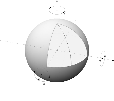
(a) $l=2$

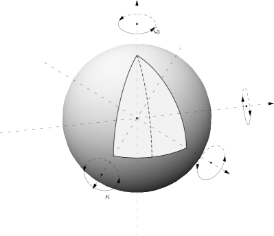
(b) $l=3$

Figure 1: Dihedral groups $D_{l}$, with the upper half of the fundamental domains in white.

The action of $D_{l}$, restricted on the fixed subspace $\left(\mathbb{R}^{4l}\right)^{D_{l}}\cong\mathbb{R}^{2}$, generates a dihedral configuration of vortices for any given ${\bm{q}}_{0}\in\mathbb{R}^{2}$. If we assign the same circulation to all vortices, then we can express the logarithmic potential acting on a single vortex as

(13) $$U({\bm{q}}_{0})=-\sum_{g\in D_{l}\smallsetminus\{1\}}\log(\left\|{\bm{q}}_{0}-g{\bm{q}}_{0}\right\|),$$

where, without further loss of generality, we have taken $\tilde{\Gamma}_{i}^{2}=2\pi/l$. A solution of equations (5) such that the vortices lie on a dihedral configuration at all times, is a dihedral equivariant orbit.

Lemma 2.1

The angular momentum of any dihedral equivariant orbit is zero.

Proof.  Using (8) and Hamilton’s equations (5), it follows that the angular momentum is:

$${\bm{M}}\,=\,\sum_{j=1}^{N}\,\hat{\bm{q}}_{j}\times\dot{\hat{\bm{q}}}_{j}.$$

By hypothesis, at each instant the configuration of the vortices is given by the action of the dihedral group $D_{l}$; ${\bm{q}}_{j}=g_{j}{\bm{q}}$ for $g_{j}\in D_{l}$. Hence

$$\hat{\bm{q}}_{j}\times\dot{\hat{\bm{q}}}_{j}=g_{j}\hat{\bm{q}}\times g_{j}\dot{\hat{\bm{q}}}\,=\,g_{j}\big{(}\hat{\bm{q}}\times\dot{\hat{\bm{q}}}\big{)}.$$

We observe that $\hat{\bm{q}}\times\dot{\hat{\bm{q}}}=(0,0,y)$, for some real number $y$. Therefore, using (2), we have

$${\bm{M}}=\sum_{j=1}^{2l}g_{j}\big{(}\hat{\bm{q}}\times\dot{\hat{\bm{q}}}\big{)}=l(0,0,y)+l(0,0,-y)={\bm{0}}.$$

This conclude the proof. $\Box$

Remark 2.2

As consequence of the Sundman-type estimates proved by authors in [BaFeTe08], for a large class of potentials including the logarithmic one, a necessary condition in order to have the total collapse is that the total angular momentum of the system should be zero. Therefore as direct consequence of Lemma 2.1, we can conclude that total collision orbits can occur.

2.1 The logarithmic dihedral potential

For $z=\rho\,e^{i\alpha}$, with $\rho\geq 0$ and $\alpha_{j}=2\pi j/l$, $j=1,\ldots,l-1$, it is easy to verify that:

$$|z-\bar{z}| =2\rho\left|\sin\alpha\right|$$

$$|z-\zeta_{l}^{j}z| =2\rho\left|\sin\left(\dfrac{\alpha_{j}}{2}\right)\right|$$

$$|z-\zeta_{l}^{j}\bar{z}| =2\rho\left|\sin\left(\dfrac{\alpha_{j}-2\alpha}{2}\right)\right|.$$

Therefore, for $\alpha\in(0,\pi/l)$ (that is, for ${\bm{q}}$ in the fundamental domain) the potential (13) becomes:

(14) $$U(\rho,\alpha):=-\log\left((2\rho)^{2l-1}\right)-\log\left[\sin\alpha\,\prod_{j=1}^{l-1}\sin\left(\dfrac{\alpha_{j}}{2}\right)\,\sin\left(\dfrac{\alpha_{j}}{2}-\alpha\right)\right].$$

Since $\prod_{j=1}^{l-1}\sin\left(j\dfrac{\pi}{l}\right)=\dfrac{l}{2^{l-1}}$ and by taking into account the multiple-angle formula

$$\sin(nx)=2^{n-1}\prod_{k=0}^{n-1}\sin\left(\dfrac{k\pi}{n}+x\right),$$

we have

$$\sin\alpha\prod_{j=1}^{l-1}\sin\left(\dfrac{j\pi}{l}-\alpha\right)=\dfrac{\sin(l\alpha)}{2^{l-1}}.$$

These calculations lead to the following definition.

Definition 2.3

We define the dihedral logarithmic potential as :

(15) $$U({\bm{q}}):=-\log\rho^{2l-1}-\log\left(2l\sin(l\,\alpha)\right),$$

and its angular part as:

(16) $$U(\alpha):=-\log\left(2l\sin(l\,\alpha)\right).$$

Lemma 2.4

(Planar $2l$-gon) The dihedral problem admits exactly one (up to permutation of the vortices) central configuration, which is given by the vertices $(e^{(2k+1)\pi i/(2l)},0)$ of a regular $2l$-gon.

Proof.  From the definition (1.1) it follows that central configuration corresponds to a critical point of the potential restricted to the shape sphere. From (16) it follows that

$$U^{\prime}(\alpha)=-\dfrac{l\,\cos(l\alpha)}{\sin(l\alpha)}$$

whose critical point in the fundamental domain of the shape sphere is $\alpha_{c}=\dfrac{\pi}{2l}$. From $U^{\prime\prime}(\alpha_{c})=l^{2}$ it also follows that the point $\alpha_{c}$ is a minimum. $\Box$
We also observe that

1. $U(\alpha_{c})<0$ for $l=2,3$;

2. $U(\alpha_{c})>0$ for $l\geq 4$.

By using the identity

$$\sin(n\alpha)=\sum_{k=0}^{n}\binom{n}{k}\cos^{k}\alpha\sin^{n-k}\alpha\sin\left(\dfrac{1}{2}(n-k)\pi\right),$$

the expression (16) may be written in terms of the local parameterization of the unit sphere ${\bm{s}}(\alpha)=(s_{1},s_{2}):=(\cos\alpha,\sin\alpha)$ as follows

(17) $$U({\bm{s}})=-\log\left[2l\sum_{j=0}^{l}\binom{l}{j}s_{1}^{j}s_{2}^{l-j}\sin\left(\dfrac{\pi}{2}(l-j)\right)\right].$$

For $j\in{\bf 2}$, $q_{j}=s_{j}\|{\bm{q}}\|$ and hence the dihedral potential given in definition 2.3 becomes:

(18) $$U({\bm{q}})=-\log\left[2l\sum_{j=0}^{l}\binom{l}{j}\|{\bm{q}}\|^{l-1}q_{1}^{j}q_{2}^{l-j}\sin\left(\dfrac{\pi}{2}(l-j)\right)\right].$$

2.2 The geometry of the energy hypersurfaces

From (10) let us define $\hat{E}(h,r,{\bm{s}}):=2r^{2}(h+U(re^{-1/r^{2}}{\bm{s}}))$. More explicitly $\hat{E}$ is given by:

$$\hat{E}(h,r,{\bm{s}}):=E(h,r)+2r^{2}\,U({\bm{s}}),$$

where $E$ is given by

(19) $$E(h,r):=2\left[h\,r^{2}+(2l-1)(1-r^{2}\log r)\right].$$

Remark 2.5

The boundary of the regions where the motion occurs is given by $\hat{E}(h,r,\alpha)=0$; more precisely, since the kinetic term $\langle\Gamma^{-1}{\bm{z}},{\bm{z}}\rangle$ is a positive definite quadratic form, for any fixed energy level $h$ the motion is possible where:

$$\hat{E}(h,r,\alpha)\,:=\,2\left[h\,r^{2}+(2l-1)(1-r^{2}\log r)\right]-2r^{2}\log(2l\sin(l\alpha))\geq\,0.$$

The shape of the curve $\hat{E}(h,r,\alpha)=0$ is key in order to understand the dynamics of our problem.

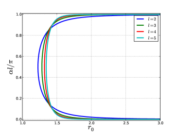
Figure 2: Zero set of the function $(r,\alpha)\mapsto\hat{E}(0,r,\alpha)$ and different value of the total number of point vortex.

Therefore the hypersurface corresponding to the energy level $h$ is given by

(20) $$\Sigma_{h}=\left\{{(r,\alpha,{\bm{z}})\in\mathbb{R}^{*}_{+}\times(0,\pi/l)\times\mathbb{R}^{2}}\mid{\langle\Gamma^{-1}{\bm{z}},{\bm{z}}\rangle\,=\,\hat{E}(h,r,\alpha)}\right\}.$$

We also observe that $\Sigma_{h}$ meets the boundary $r=0$ along a submanifold given by

$$\Lambda:=\left\{{(0,\alpha,{\bm{z}})\in\mathbb{R}^{*}_{+}\times(0,\pi/l)\times\mathbb{R}^{2}}\mid{\langle\Gamma^{-1}{\bm{z}},{\bm{z}}\rangle\,=\,2\,(2l-1)}\right\}.$$

The set $\Lambda$ is diffeomorphic to an open cylinder and it represents the component over the fundamental domain of the total collision manifold. As we shall see in the following, the total collision manifold is homeomorphic to a two dimensional torus.

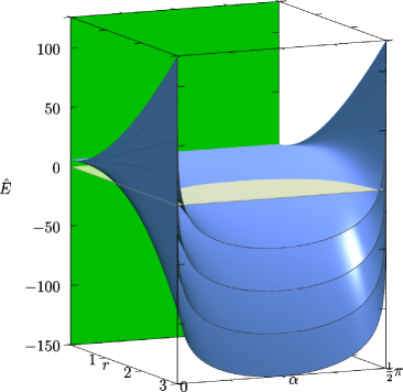
Figure 3: Energy hypersurfaces for different values of the energy level $h$ and the zero plane.

Let us introduce a further change of coordinates. In the dihedral problem the shape sphere reduces to $S^{1}$, therefore it is natural to use the parameterization $\alpha\mapsto{\bm{s}}(\alpha)$, where ${\bm{s}}(\alpha)=(\cos\alpha,\sin\alpha)$. Following [StFo03], we exploit the constraint (20) to parameterize the we also introduce a new local parameterization the momentum coordinates ${\bm{z}}$ with an angle $\psi$ in the following way

(21) $${\bm{z}}=\sqrt{\hat{E}(h,r,\alpha)}\,(\sqrt{\frac{2\pi}{l}}\cos\psi,\sqrt{\frac{2\pi}{l}}\sin\psi).$$

Note that with the choice of the strength of the circulations made in Section 2, we have $\Gamma^{-1}=l/2\pi I$. We also use a new time-like variable $\zeta$, defined by

$$d\tau=\sqrt{\hat{E}}\,d\zeta.$$

With the above parameterizations, the system (12) reduces to

(22) $$\left\{\begin{array}[]{ll}\dfrac{dr}{d\zeta}=\sqrt{\dfrac{l}{2\pi}}\dfrac{r^{3}}{r^{2}+2}\,\hat{E}(h,r,\alpha)\,(\cos\alpha\cos\psi+\sin\alpha\sin\psi)\\ \\ \dfrac{d\alpha}{d\zeta}=\sqrt{\dfrac{l}{2\pi}}\hat{E}(h,r,\alpha)(\sin\psi\cos\alpha-\sin\alpha\cos\psi)\\ \\ \dfrac{d\psi}{d\zeta}=\sqrt{\dfrac{l}{2\pi}}r^{2}(\partial_{q_{2}}U({\bm{s}}(\alpha))\,\cos\psi-\partial_{q_{1}}U({\bm{s}}(\alpha))\sin\psi).\\ \end{array}\right.$$

The following result is an obvious consequence of equations (22).

Lemma 2.6

The collision manifold at $r=0$ and the zero velocity manifold $\hat{E}(h,r,\alpha)=0$ are invariant manifolds. Moreover:

1. On the collision manifold $r=0$ the dynamics is given by

   $$\dfrac{d\alpha}{d\zeta}=-\sqrt{\dfrac{l}{2\pi}}2(2l-1)\sin(\psi-\alpha),\qquad\dfrac{d\psi}{d\zeta}=0;$$

2. On the zero-velocity manifold $\hat{E}(h,r,\alpha)=0$, the dynamics is obtained by integrating the last equation in (22), keeping $r,$ $\alpha$ as constants.

3 Flow and invariant manifolds: the Klein group $D_{2}$

For $l=2$ (the Klein group) we may carry out a detailed study of the global dynamic of the problem. We observe that the dihedral potential reduces to:

$$U({\bm{q}})=-\log(8\|{\bm{q}}\|q_{1}q_{2})$$

whence it follows $\partial_{{\bm{q}}}U({\bm{s}})=-\left(\dfrac{1}{s_{1}}+s_{1},\dfrac{1}{s_{2}}+s_{2}\right).$ In this case the equations of motion become:

(23) $$\left\{\begin{array}[]{ll}\dfrac{dr}{d\zeta}=\dfrac{1}{\sqrt{\pi}}\dfrac{r^{3}}{r^{2}+2}\,\hat{E}(h,r,\alpha)\,\cos(\psi-\alpha)\\ \\ \dfrac{d\alpha}{d\zeta}=\dfrac{1}{\sqrt{\pi}}\hat{E}(h,r,\alpha)\,\sin(\psi-\alpha)\\ \\ \dfrac{d\psi}{d\zeta}=\dfrac{-r^{2}}{\sqrt{\pi}}\left[\dfrac{2\cos(\psi+\alpha)}{\sin 2\alpha}-\sin(\psi-\alpha)\right].\end{array}\right.$$

The rest points of (23) correspond to the solutions of the following systems:

$$\left\{\begin{array}[]{ll}r=0\\ \sin(\psi-\alpha)=0\end{array}\right.,\qquad\left\{\begin{array}[]{ll}r=0\\ \hat{E}=0\end{array}\right.,\qquad\left\{\begin{array}[]{ll}\hat{E}=0\\ \dfrac{2\cos(\psi+\alpha)}{\sin 2\alpha}=\sin(\psi-\alpha)\end{array}\right..$$

However, it is readily seen that the second system has no solutions, as the conditions $\hat{E}=0$ and $r=0$ are incompatible. With straightforward calculations we obtain the following result.

Lemma 3.1

The equilibria of the vector field given in (23) consists of four curves, two belonging to the collision manifold and the other two on the zero-velocity manifold. In the coordinates $(r,\alpha,\psi)$, the curves on the collision manifold are given by

1. $\mathscr{P}_{1}\equiv(0,\alpha,\alpha)$;

2. $\mathscr{P}_{2}\equiv(0,\alpha,\alpha+\pi)$

The curves on the zero-velocity manifold are given by

1. $\mathscr{P}_{3}\equiv\big{(}r,\alpha,\arctan m(\alpha)\big{)}$;

2. $\mathscr{P}_{4}\equiv\big{(}r,\alpha,\arctan m(\alpha)+\pi\big{)}$, where

   $$m(\alpha):=\dfrac{\cos\alpha(\sin^{2}\alpha+1)}{\sin\alpha(\cos^{2}\alpha+1)}.$$

   and the pair $(r,\alpha)$ satisfies the equation $\hat{E}(h,r,\alpha)=0$, which explicitly reads

   $$\log(4\sin 2\alpha)=h+3(r^{-2}-\log r).$$

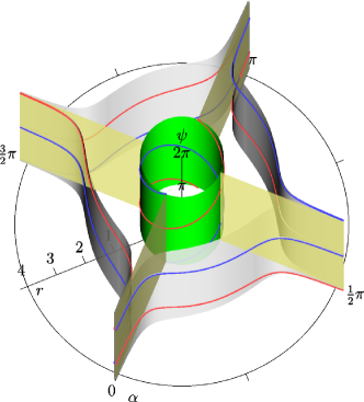
Figure 4: Rest points and invariant manifolds for the $D_{2}$ problem. The green cylinder is the total collision manifold $r=0$; the blue and the red lines lying on it are $\mathscr{P}_{1}$ and $\mathscr{P}_{2}$, respectively. The four light grey manifolds are the surfaces defined by $\hat{E}(0,r,\alpha)=0$ (there is one for each of the four domains of the group $D_{2}$); the red and the blue lines lying on them are $\mathscr{P}_{3}$ and $\mathscr{P}_{4}$ in the fundamental domain, and their images in the other domains. The blue/red color denotes families of rest points which are transversally linearly stable/unstable on their own invariant surface. See the text for the stability in directions transverse to the invariant surfaces. The four yellow planes correspond to binary collisions.

The spectrum and the eigenvectors of the Jacobian matrix of (23), evaluated at a rest point, gives useful information on the local dynamics close to the curves $\mathscr{P}_{1}$, $\mathscr{P}_{2}$, $\mathscr{P}_{3}$, $\mathscr{P}_{4}$. The logic of the calculation is elementary, but the computations occasionally become too large to be easily manageable. With the help of a computer algebra system (Maxima 5.21.1) we arrive at the following results.

Lemma 3.2

The curves of equilibria $\mathscr{P}_{1}$ and $\mathscr{P}_{2}$ (on the collision manifold) given in Lemma 3.1 are degenerate. More precisely:

1. at each point of the curve $\mathscr{P}_{1}$ the spectrum is given by $\mathfrak{s}(\mathscr{P}_{1})=\{\lambda_{1},\lambda_{2}\}$ where $\lambda_{1}=6/\sqrt{\pi}$ and $\lambda_{2}=0$. Furthermore the algebraic multiplicity of $\lambda_{1}$ is $h(\lambda_{1})=1$ and the algebraic multiplicity of $\lambda_{2}$ is $h(\lambda_{2})=2$. The eigenvectors are

   $${\bm{v}}_{1}=(0,1,0)\ \ {\bm{v}}_{2}=(1,0,0)\ \ {\bm{v}}_{3}=(0,1,1)$$

   where ${\bm{v}}_{1}$ is associated to $\lambda_{1}$ and ${\bm{v}}_{2}$, ${\bm{v}}_{3}$ are associated to $\lambda_{2}$. The vector ${\bm{v}}_{3}$ is tangent to $\mathscr{P}_{1}$.

2. At each point of the curve $\mathscr{P}_{2}$ the spectrum is given by $\mathfrak{s}(\mathscr{P}_{2})=\{\lambda_{1},\lambda_{2}\}$ where $\lambda_{1}=-6/\sqrt{\pi}$ and $\lambda_{2}=0$. The multiplicities and the eigenvectors are the same as for $\mathscr{P}_{1}$.

Lemma 3.3

The curves of equilibria $\mathscr{P}_{3}$ and $\mathscr{P}_{4}$ (on the zero velocity manifold) given in Lemma 3.1 are degenerate. More precisely:

1. at each point of the curve $\mathscr{P}_{3}$ the spectrum is given by three distinct simple eigenvalues, namely $\mathfrak{s}(\mathscr{P}_{3})=\{\mu_{1},\mu_{2},\mu_{3}\}$ where

   $$\begin{split}\mu_{1}&=0\\ \mu_{2}&=-\dfrac{2r^{2}\,\big{[}3\,\cos(\psi-\alpha)e^{6/r^{2}+2h}+64\,\cos(2\alpha)\,\cos(\psi+\alpha)r^{6}\big{]}}{e^{6/r^{2}+2h}\,\sqrt{\pi}}\\ \mu_{3}&=\dfrac{r^{2}\big{[}\cos(\psi-\alpha)\,e^{3/r^{2}+h}+8\sin(\psi+\alpha)\,r^{3}\big{]}}{e^{3/r^{2}+h}\,\sqrt{\pi}},\end{split}$$

   and

   $$\hat{E}_{0}(r,\alpha)=0,\qquad\dfrac{2\cos(\psi+\alpha)}{\sin 2\alpha}=\sin(\psi-\alpha).$$

   The eigenvector associated to $\mu_{3}$ is ${\bm{u}}_{3}=(0,0,1)$, which lies on the invariant manifold $\hat{E}(h,r,\alpha)=0$. The explicit expressions of the eigenvectors ${\bm{u}}_{1}$ and ${\bm{u}}_{2}$ associated to $\mu_{1}$ and to $\mu_{2}$ are not short, and we omit them. However, ${\bm{u}}_{1}$ is tangent to the curve $\mathscr{P}_{3}$ and ${\bm{u}}_{2}$ is transverse to $\hat{E}(h,r,\alpha)=0$.

2. At each point of the curve $\mathscr{P}_{4}$ the spectrum is $\mathfrak{s}(\mathscr{P}_{3})=\{\mu_{1},-\mu_{2},-\mu_{3}\}$. The eigenvectors are the same as for $\mathscr{P}_{3}$.

Remark 3.4

For any $\alpha\in(0,\pi/2)$ it is $\mu_{2}<0$ and $\mu_{3}>0$. In fact, from the explicit expression of $\psi(\alpha)$ given in (3.1) we have $\cos(\psi-\alpha)>0$, $\sin(\psi+\alpha)>0$, $\cos(2\alpha)\cos(\psi+\alpha)>0$. The last inequality stems from

$$\begin{split}\pi/4<\psi(\alpha)<\pi/2-\alpha\quad\mathrm{if}\quad\hphantom{\pi/}0<\alpha<\pi/4;\\ \pi/4>\psi(\alpha)>\pi/2-\alpha\quad\mathrm{if}\quad\pi/4>\alpha>\pi/2.\end{split}$$

Remark 3.5

The above results show that the stability properties of the equilibria do not depend on the value of the total energy $h$. In other words, changing the parameter $h$ does not lead to bifurcations.

At each rest point let us denote by $W^{s}$, $W^{u}$ respectively the (linearly) stable and unstable manifolds, and by $W^{0}$ the center manifold. The following results hold.

Proposition 3.6

Any rest point in $\mathscr{P}_{3}$ and $\mathscr{P}_{4}$ is a degenerate saddle. More precisely we have

1. $\dim W^{u}(\mathscr{P}_{3})=1,\qquad\dim W^{s}(\mathscr{P}_{3})=1,\qquad\dim W^{0}(\mathscr{P}_{3})=1.$

2. $\dim W^{u}(\mathscr{P}_{4})=1,\qquad\dim W^{s}(\mathscr{P}_{4})=1,\qquad\dim W^{0}(\mathscr{P}_{4})=1.$

Proof.  The statement is an immediate consequence of Lemma 3.2. Note that $\mathscr{P}_{3}$ and $\mathscr{P}_{4}$ are the center manifold of each of their own points, and that they are neutral, in the sense that each of their points is an equilibrium. $\Box$

	$\dim W^{s}\$	$\dim W^{u}\$	$\dim W^{0}\$
At $\mathscr{P}_{1}$	$1$	–	$2$
At $\mathscr{P}_{2}$	–	$1$	$2$
At $\mathscr{P}_{3}$	$1$	$1$	$1$
At $\mathscr{P}_{4}$	$1$	$1$	$1$

Table 1: Dimensions of the invariant manifolds for the equilibria belonging to the curves $\mathscr{P}_{1}$, $\mathscr{P}_{2}$, $\mathscr{P}_{3}$, $\mathscr{P}_{4}$

Proposition 3.7

For each $\alpha$, the two equilibria

$$(0,\alpha,\alpha)\in\mathscr{P}_{1}$$

and

$$(0,\alpha,\alpha+\pi)\in\mathscr{P}_{2}$$

are nonlinear degenerate saddles.

1. $\dim W^{s}(\mathscr{P}_{1})\hphantom{{}^{c}}=1,\qquad\dim W^{0}(\mathscr{P}_{1})=2.$

2. $\dim W^{u}(\mathscr{P}_{2})\hphantom{{}^{c}}=1,\qquad\dim W^{0}(\mathscr{P}_{2})=2.$

Proof.  The equations of motion for an initial condition on the collision manifold reduce to

(24) $$\left\{\begin{array}[]{lll}\dfrac{dr}{d\zeta}=0\\ \\ \dfrac{d\alpha}{d\zeta}=\dfrac{6}{\sqrt{\pi}}\,\sin(\psi-\alpha)\\ \\ \dfrac{d\psi}{d\zeta}=0.\\ \end{array}\right.$$

It is then evident that the unstable manifold of the equilibrium $(0,\alpha_{0},\alpha_{0})\in\mathscr{P}_{1}$ is the line $(0,\alpha,\alpha_{0})$, and analogously $(0,\alpha,\alpha_{0}+\pi)$ is the stable manifold for any point $(0,\alpha_{0},\alpha_{0}+\pi)\in\mathscr{P}_{2}$.

The linear stability analysis of Lemma 3.2 shows that each point on $\mathscr{P}_{1}$ and $\mathscr{P}_{2}$ has a two-dimensional center subspace, and hence a two-dimensional center manifold. In fact $\mathscr{P}_{1}$ and $\mathscr{P}_{2}$ are neutral submanifolds of the center manifold, in the sense that each of its points is an equilibrium.

For brevity, here we shall not perform a formal center manifold reduction. In order to determine the stability of the dynamics on the center manifold we simply observe that the dynamics projected along the direction singled out by the eigenvalue ${\bm{v}}_{2}=(1,0,0)$, which is transverse to the total collision manifold, is given by the first equation in (23). From that, we have $dr/d\zeta>0$ in a neighborhood of any point of $\mathscr{P}_{1}$ and $dr/d\zeta<0$ in a neighborhood of any point of $\mathscr{P}_{2}$.

Therefore the equilibria of both $\mathscr{P}_{1}$ and $\mathscr{P}_{2}$ are nonlinear saddles. $\Box$

4 Heteroclinic connections and homothetic orbits

The existence of heteroclinic connections on and between the invariant manifolds helps us to develop a global understanding of the flow.

Lemma 4.1

The flow on the total collision manifold is totally degenerate. That is:

1. $W^{u}({\bm{P}}_{1})\equiv W^{s}({\bm{P}}_{2})$;

2. $W^{u}({\bm{P}}_{2})\equiv W^{s}({\bm{P}}_{1})$;

where ${\bm{P}}_{1}\in\mathscr{P}_{1}$ and ${\bm{P}}_{2}\in\mathscr{P}_{2}$ are chosen in such a way that the second coordinate of the two points is the same.

Proof.  The proof of this result follows by a straightforward integration of the equations of motion (24) valid on the total collision manifold $r=0$. Note that the singularity of the potential at $\alpha=j\pi/4$, $j=0,\cdots,3$ vanishes on the total collision manifold, therefore on the heteroclinic connection between ${\bm{P}}_{1}$ and ${\bm{P}}_{2}$, we have $\alpha\in[0,2\pi)$. $\Box$

Remark 4.2

By taking into account the identification of the opposite edges of the rectangle $(\alpha,\psi)$ with the same orientation, the curves of equilibria can be identified with two closed curves on the torus and the heteroclinics are represented by arcs joining one point on a unstable (red) closed curve with the corresponding point on the stable (blue) curve as shown in Figure (5).

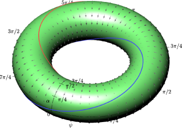
Figure 5: Total collision manifold and equilibrium curves.

Next we describe the flow on the zero velocity manifold $\hat{E}(h,r,\alpha)=0$, where the equations of motion reduce to

(25) $$\dfrac{dr}{d\zeta}=0,\quad\dfrac{d\alpha}{d\zeta}=0,\quad\dfrac{d\psi}{d\zeta}=-\dfrac{r^{2}}{\sqrt{\pi}}\,\left[\dfrac{2\cos(\psi+\alpha)}{\sin 2\alpha}-\sin(\psi-\alpha)\right].$$

Lemma 4.3

The flow on the total collision manifold is totally degenerate. More precisely

1. $W^{u}({\bm{P}}_{3})\equiv W^{s}({\bm{P}}_{4})$;

2. $W^{u}({\bm{P}}_{4})\equiv W^{s}({\bm{P}}_{3})$;

where ${\bm{P}}_{3}\in\mathscr{P}_{3}$ and ${\bm{P}}_{4}\in\mathscr{P}_{4}$ are chosen in such a way that the first two coordinates agree.

Proof.  From Lemma 3.1 we have ${\bm{P}}_{4}={\bm{P}}_{3}+(0,0,\pi)$. From the equations of motion (25) follows that the flow lines on $\hat{E}(h,r,\alpha)=0$ are straight lines parallel to the $\psi$-axis. Therefore they are heteroclinic connections between each point ${\bm{P}}_{3}\in\mathscr{P}_{3}$ and the corresponding ${\bm{P}}_{4}\in\mathscr{P}_{4}$. $\Box$

By choosing $(\alpha,\psi)=(\pi/4,\pi+\pi/4)$ or $(\alpha,\psi)=(\pi/4,\pi/4)$ the last two equations in (23) are identically zero. This means that the constant pair $(\alpha,\psi)=(\pi/4,\pi+\pi/4)$ is a constant solution of the subsystem obtained by projecting the system of ode’s onto the $(\alpha,\psi)$-plane. By summing up, the following result holds.

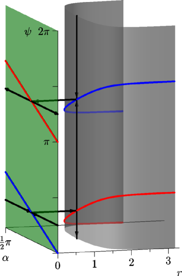
Figure 6: Heteroclinic connections among the points $(0,\pi/4,\pi/4)$, $(0,\pi/4,\pi+\pi/4)$, $(\bar{r},\pi/4,\pi/4)$, $(\bar{r},\pi/4,\pi+\pi/4)$ where $\bar{r}$ is such that $\hat{E}(h,\bar{r},\pi/4)=0$.

Proposition 4.4

There exist two connecting orbits between the total collision and zero velocity manifold. More precisely

1. The curve $\eta_{13}(\zeta)=\big{(}r(\zeta),\pi/4,\pi/4\big{)}$ is an heteroclinic joining $\mathscr{P}_{1}$ and $\mathscr{P}_{3}$ for $r$ solution of

   $$\dfrac{dr}{d\zeta}=\dfrac{1}{\sqrt{\pi}}\dfrac{r^{3}}{r^{2}+2}\,\hat{E}(h,r,\pi/4).$$

2. the curve $\eta_{24}(\zeta)=\big{(}r(\zeta),\pi/4,\pi+\pi/4\big{)}$ is an heteroclinic joining $\mathscr{P}_{4}$ and $\mathscr{P}_{2}$ for $r$ solution of

   $$\dfrac{dr}{d\zeta}=-\dfrac{1}{\sqrt{\pi}}\dfrac{r^{3}}{r^{2}+2}\,\hat{E}(h,r,\pi/4).$$

where $\hat{E}(h,r,\pi/4)=2[hr^{2}+3(1-r^{2}\log r)]-2r^{2}\log 4$.

Remark 4.5

From Lemma 2.4 with $l=2$ it follows that the heteroclinic connections $\eta_{13}$ and $\eta_{24}$ are self–similar orbits where the vortices are located at the vertices of a square. Their projection on the shape sphere is a central configuration. Moreover, these are the only self–similar orbits: from (23) it follows that no other solution curve has $\alpha(\zeta)=\pi/4$ when $\zeta$ ranges on an interval of non–zero length.

Remark 4.6

A classical result of Sundman [Sun09] proved for the three-body problem in three dimensions that an orbit ending in triple collision asymptotically approaches a central configuration. The validity of Sundman-type asymptotic estimates for collision solutions is established in a recent paper [BaFeTe08, Theorem 5, Example2] for a wide class of dynamical systems with singular forces, including the classical $N$-body problem, quasi-homogeneous and logarithmic potentials. Applying these results to our problem, we deduce that the only point of the total collision manifold which is (asymptotically) reachable by an orbit originating from an initial condition having $r>0$ is $(r,\alpha,\psi)=(0,\pi/4,5\pi/4)$, while $(r,\alpha,\psi)=(0,\pi/4,\pi/4)$, is the only point reachable extending the orbit backward in time. In this sense, the collision manifold, with the exception of these two points, is dynamically disconnected from the region $r>0$.

Figure 6 shows graphycally the heteroclinic connections between the invariant manifolds $r=0$ and $\hat{E}=0$.

Remark 4.7

We stress that, while an initial condition on the heteroclinic $\eta_{13}$ is unable to complete the loop up to the total collision manifold (it just asymptotically reaches a fixed point on $\mathscr{P}_{3}$), the dynamics expressed in Cartesian coordinates by (5) does perform the loop in a finite time. In fact, the points on the curves $\mathscr{P}_{3}$ and $\mathscr{P}_{4}$ of the zero velocity manifolds appear as rest points in McGehee coordinates just because the time transformation (2.2) is singular when $\hat{E}(h,r,\alpha)=0$. Their counterparts in Cartesian coordinates correspond to turning points where $\dot{{\bm{q}}}(\sigma)=\bm{0}$

5 Global dynamics in McGehee coordinates

The typical orbit of equations (23) experiences a binary collision within a finite time, as we shall prove in this section. The exceptions constitute a set of zero Lebesgue measure. Moreover, there are no unbounded orbits, even when one introduces generalized solutions that allow for an orbit to pass through a binary collision.

5.1 Non-existence of unbounded non-colliding trajectories

Let us start by ruling out unbounded, collisionless orbits. In our problem orbits escaping to infinity cannot be ruled out with a simple argument based on the conservation of total energy $h$, because for any given $h$ the distance $r$ from the center of vorticity may grow without bounds while maintaining the same positive value of the (rescaled) kinetic energy $\hat{E}$, as should be apparent from Figures 3 and 2.

Definition 5.1

We say that a solution $\gamma(\zeta):=(r(\zeta),\alpha(\zeta),\psi(\zeta))$ of the system (23) is unbounded if

$$\lim_{\zeta\to+\infty}r(\zeta)=+\infty$$

Theorem 5.2

Equations (23) do not allow for unbounded collisionless orbit.

Proof.  Let us consider the system (23); eliminating the time variable $\zeta$ this system is equivalent to

(26) $$\left\{\begin{array}[]{ll}\dfrac{d\alpha}{dr}=-\dfrac{r^{2}+2}{r^{3}}\,\tan(\psi-\alpha)\\ \\ \dfrac{d\psi}{dr}=-\dfrac{r^{2}+2}{r\hat{E}}\left[\dfrac{2\cos(\psi+\alpha)}{\sin(2\alpha)\,\cos(\psi-\alpha)}-\tan(\psi-\alpha)\right]\end{array}\right.$$

By contradiction, we assume that there exists an unbounded motion $r\mapsto(\alpha(r),\psi(r))$ starting from the initial condition ${\bm{h}}_{0}=(r_{0},\alpha_{0},\psi_{0})$ and we suppose that the orthogonal projection of ${\bm{h}}_{0}$ onto the $(r,\alpha)$-plane is a point $\hat{\bm{h}}_{0}$ lying in the region between the straight lines $\alpha=0$, $r=r_{*}$ and the zero set of the function $\hat{E}$, where $r_{*}$ is such that $\hat{E}_{0}(r_{*},\pi/4)=0$ (see Figure 2). The case where $\hat{\bm{h}}_{0}$ lies between the straight lines $\alpha=\pi/2$, $r=r_{*}$ and the zero set of the function $\hat{E}$ is analogous and will not be explicitly addressed. In order to maintain $\hat{E}>0$, an unbounded motion must satisfy

(27) $$0<\alpha(r)<g(r),\qquad\textrm{where}\quad g(r):=\dfrac{1}{2}\arcsin\left[\dfrac{1}{4}\,\exp\left(\dfrac{E_{0}(r)}{2\,r^{2}}\right)\right]$$

for $E_{0}(r)=6(1-r^{2}\log r)$. We observe that

$$\lim_{r\to+\infty}E_{0}(r)/2r^{2}=\lim_{r\to+\infty}\log r^{-3}=-\infty,$$

from which it follows that $g(r)\sim_{+\infty}1/(8r^{3})+o(1/r^{4})$. Thus $r\mapsto\alpha(r)$ decreases to zero at infinity while keeping $r\mapsto g(r)$ as an upper bound. From the first equation in (26) we have

$$\dfrac{d\alpha}{dr}=-\dfrac{r^{2}+2}{r^{2}}\dfrac{\tan(\psi(r)-\alpha(r))}{r}\sim_{+\infty}-\dfrac{\tan(\psi(r)-\alpha(r))}{r}.$$

and therefore

$$\lim_{r\to+\infty}\dfrac{\tan(\psi(r)-\alpha(r))}{r}=0,$$

We conclude that the function $r\mapsto\alpha(r)$ should satisfy the limit equation

$$\dfrac{d\alpha}{dr}=-\dfrac{\tan(\psi(r))}{r}.$$

From the second equation in (26) we have

$$\dfrac{d\psi}{dr}=-\dfrac{r^{2}+2}{r\hat{E}}\left[\dfrac{2\cos(\psi+\alpha)}{\sin(2\alpha)\cos(\psi-\alpha)}-\tan(\psi-\alpha)\right]\sim_{+\infty}-\dfrac{r}{\hat{E}}\left[\dfrac{1}{\alpha}-\tan\psi\right].$$

From the upper bound $r\mapsto\alpha(r)\in O(1/r^{3})$ we also have

$$\hat{E}(h,r,\alpha)\sim_{+\infty}-6r^{2}\log r+o(r^{2}\log r).$$

Therefore an unbounded motion should satisfy the limit problem

$$(\mathscr{P}_{\infty})\ \quad\left\{\begin{array}[]{ll}\dfrac{d\alpha}{dr}=-\dfrac{\tan\psi}{r}\\ \\ \dfrac{d\psi}{dr}=\dfrac{1}{6r\log r}\left[\dfrac{1}{\alpha}-\tan\psi\right].\end{array}\right.$$

The first equation is equivalent to

$$\psi(r)=-\arctan(r\alpha^{\prime})$$

hence unbounded orbits should asymptotically satisfy the following second order differential equation

(28) $$-\dfrac{\alpha^{\prime}+r\alpha^{\prime\prime}}{1+r^{2}\alpha^{\prime 2}}=\dfrac{1}{6r\log r}\left[\dfrac{1+r\alpha\,\alpha^{\prime}}{\alpha}\right].$$

Multiplying the equation by $\alpha$ and taking into account that both $\alpha$ and $\alpha^{\prime}$ go to zero as $r\to+\infty$ it follows that the above equation reduces to

$$\alpha\alpha^{\prime\prime}=-\dfrac{1}{6r^{2}\log r}.$$

Observing that $\alpha>0$, it follows that an unbounded solution should be concave, which contradicts the inequality (27). $\Box$

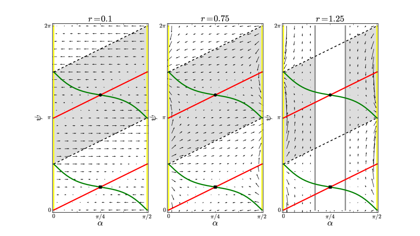
Figure 7: Projection of the vector field in equation (23) on the $(\alpha,\psi)$ plane at three different values of $r$. The black square and circle are, respectively the intersection with the plane of the ejection and collision heterocline of Proposition 4.4. The yellow vertical lines show the binary-collision planes at $\alpha=0$ and $\alpha=\pi/2$. The red and green lines are, respectively, the places where $d\alpha/d\zeta=0$ and $d\psi/d\zeta=0$. The vertical grey lines show the intersection of the zero velocity manifold $\hat{E}=0$ with the plane $r=1.25$. The vector field is not shown in the dynamically meaningless region between the two lines, where $\hat{E}<0$. The regions shaded in light grey are those where $dr/d\zeta<0$. Elsewhere it is $dr/d\zeta>0$, except along the black dashed lines, where $dr/d\zeta=0$.

5.2 Generality of binary collisions

Theorem 5.3

Any orbit not fully contained in the total collision manifold or in the zero velocity manifold, or in the central manifold of the rest point $(r,\alpha,\psi)=(0,\pi/4,5\pi/4)$ or in the stable manifold of the rest points $\mathscr{P}_{3}$ experiences a binary collision. Moreover, the union of the orbits that do not experience a binary collision is a set of zero Lebesgue measure in $\mathbb{R}^{3}$.

Proof.  The total collision manifold and the zero velocity manifold are both two-dimensional, hence of zero Lebesgue measure. They are invariant manifolds and the orbits lying on them do not experience binary collisions, as illustrated in the previous section.

Of all the points on the total collision manifold, only $(r,\alpha,\psi)=(0,\pi/4,5\pi/4)$ may be reached starting from $r>0$ (Remark 4.6). The heterocline $\eta_{24}$ belongs to the central manifold of $(r,\alpha,\psi)=(0,\pi/4,5\pi/4)$ associated to the eigenvector ${\bm{v}}_{2}$ of $\mathscr{P}_{2}$ (Lemma 3.2). Owing to the non-uniqueness of the central manifold, other orbits are possible that become tangent to the heterocline $\eta_{24}$ as $r\to 0$. Defining $\phi=\psi-\alpha-\pi$, $\beta=\alpha-\pi/4$, and approximating equations (23) at first order in $\beta$, $\phi$, the dynamics of orbits arbitrarily close to the heterocline is described by

(29) $$\left\{\begin{array}[]{ll}\dfrac{dr}{d\zeta}=-\hat{E}\,\dfrac{r^{3}}{r^{2}+2}\\ \\ \dfrac{d\beta}{d\zeta}=-\hat{E}\,\phi\\ \\ \dfrac{d\phi}{d\zeta}=-r^{2}(3\phi+4\beta).\end{array}\right.$$

where we have omitted the irrelevant $\pi^{-1/2}$ factors. Here $(\beta,\phi)=(0,0)$ is the heterocline, and $r$ is a monotonically decreasing function of $\zeta$. At each fixed value $r>0$ this system of equations has a contracting and an expanding direction on the $(\beta,\phi)$-plane, associated, respectively, to the eigenvalues $\lambda_{1}=-r(\sqrt{16\hat{E}+9r^{2}}+3r)/2$ and $\lambda_{2}=r(\sqrt{16\hat{E}+9r^{2}}-3r)/2$. The contracting direction is given by the vector $(r,\beta,\phi)=(0,2\hat{E},r(\sqrt{16\hat{E}+9r^{2}}+3r))$, therefore the center manifold is a two-dimensional surface that becomes tangent to $(r,\alpha,\psi)=(r,\alpha,\alpha+\pi)$ at $(\alpha,\psi)=(\pi/4,5\pi/4)$ as $r\to 0$.

Another set of orbits that do not experience binary collisions are the stable manifolds of the points of $\mathscr{P}_{3}$ associated to the stable eigenvector ${\bm{u}}_{2}$ (Lemma 3.3). These points are normally hyperbolic, and the union of their stable manifolds is, again, a smooth two dimensional surface. See [HiPuSh77] for details.

Finally, from equations (23), in the rectangle ${\bm{R}}=(0,\pi/2)\times[0,2\pi]$ of the $(\alpha,\psi)$-plane, we have the following properties of the orbits (see also Figure 7):

• $\alpha$ increases (with respect to time $\zeta$) in the region of ${\bm{R}}$ where

  $$\alpha<\psi<\alpha+\pi$$

  and decreases otherwise;

• $\psi$ increases (with respect to time $\zeta$) in the region of ${\bm{R}}$ where

  $$\arctan(m(\alpha))<\psi<\arctan(m(\alpha))+\pi.$$

  and decreases otherwise.

• $r$ decreases (with respect to time $\zeta$) in the region of ${\bm{R}}$ where

  $$\alpha+\pi/2<\psi<\alpha+3\pi/2$$

  and decreases otherwise.

The qualitative behavior of the vector field then rules out limit cycles or other invariant structures. Theorem 5.2 shows that collisionless, unbounded orbits are impossible. It then follows that orbits not on the above mentioned invariant manifolds, whose union is a set of zero Lebesgue measure, must reach a binary collision. $\Box$

5.3 Generalized solutions: a boundedness result

As a consequence of the fact that almost every orbit experiences a binary collision, we are lead to ask if it is possible to continue the solution after a binary collision in some natural manner. This is classical question in the context of $n$-body gravitational problems and it goes under the name of regularization of collisions. Motivated by the recent paper [CaTe] we shall introduce the notion of generalized solutions which, very roughly, are the continuation of the classical solutions after the binary collision in a suitable manner. In this section all “collisions” should be intended as “binary collisions”, thus excluding the case of total collapse. Before proceeding further, we firstly recall some facts proven in [CaTe] in the case of weak central forces.

One-center problem with logarithmic potential

Let us consider the dynamical system associated with the conservative central weak force arising by a logarithmic potential having the singularity at the origin; i.e. the Cauchy problem:

(30) $$\left\{\begin{array}[]{ll}\ddot{\bm{q}}=\partial_{\bm{q}}U({\bm{q}})\\ \\ ({\bm{q}}(0),\dot{\bm{q}}(0))=({\bm{q}}_{0},{\bm{p}}_{0})\in(\mathbb{R}^{2}\setminus\{\bm{0}\}\times\mathbb{R}^{2})\end{array}\right.$$

where $U({\bm{q}}):=-\log(\|{\bm{q}}\|)$. A classical solution does not cross the singularity of the force, i.e. is a path ${\bm{q}}\in\mathscr{C}^{2}(T,\mathbb{R}^{2}\setminus\{\bm{0}\})$ where $T$ denotes the maximal interval of existence. For the classical $n$-body problem, De Giorgi in [DeG96] proposed in to consider the smoothing of the potential as a regularization technique. An exhaustive analysis in the case of homogeneous potentials, including the classical Keplerian potential, was performed by Bellettini, Fusco e Gronchi in [BaFuGr03]. Following the idea of De Giorgi, the authors in [CaTe] removed the singularity at ${\bm{q}}=0$ by smoothing the potential as follows:

$$U({\bm{q}};\varepsilon)=\log\sqrt{\|{\bm{q}}\|^{2}+\varepsilon^{2}}$$

and by considering the regularized problem

(31) $$\left\{\begin{array}[]{ll}\ddot{\bm{q}}=\partial_{\bm{q}}U({\bm{q}};\varepsilon)\\ \\ ({\bm{q}}(0),\dot{\bm{q}}(0))=({\bm{q}}_{0},{\bm{p}}_{0})\in(\mathbb{R}^{2}\times\mathbb{R}^{2})\end{array}\right.$$

Unlike in (30) the differential equation in (31) is no longer singular, so the initial value problem admits a global smooth solution ${\bm{q}}\in\mathscr{C}^{\infty}(\mathbb{R},\mathbb{R}^{2})$ for every choice of the initial value $({\bm{q}}_{0},{\bm{p}}_{0})$. Let $B_{0}(\bar{R})$ be a ball of radius $\bar{R}$ centered at the origin of the configuration space, and let $\mathscr{S}\subset\mathbb{R}^{2}\times\mathbb{R}^{2}$ be the set of initial conditions within the ball leading to collision for the problem with $\varepsilon=0$. For every $\bar{\nu}\in\mathscr{S}$ let ${\bm{q}}_{\bar{\nu}}\in\mathscr{C}^{2}(T,\mathbb{R}^{2})$ be the collision solution where $T$ denotes the maximal interval of existence. Denoting with ${\bm{q}}_{\varepsilon,\nu}$ the solution with initial data $\nu$ and studying the asymptotic limit $(\varepsilon,\nu)\to(0,\bar{\nu})$, the authors in [CaTe] introduced the following two notions of regularization.

Definition 5.4

We say that the problem (30) is weakly regularizable via smoothing of the potential in the ball $B_{0}(\bar{R})$ if, for every $\bar{\nu}\in\mathscr{S}$ there exist two sequences $(\varepsilon_{k})_{k},(\nu_{k})_{k}$ tending to $0$ and $\bar{\nu}$ respectively such that there exists

$$\lim_{k\to\infty}{\bm{q}}_{\varepsilon_{k},\nu_{k}}=\bar{\bm{q}}$$

and the flow

$$\tilde{\bm{q}}_{\nu}(t)=\left\{\begin{array}[]{ll}{\bm{q}}_{\nu}(t)&\nu\notin\mathscr{S}\\ \bar{\bm{q}}(t)&\nu\in\mathscr{S}\end{array}\right.$$

is continuous with respect to $\nu$ (i.e. the initial point).

Definition 5.5

The singular one center problem (31) is strongly regularizable via smoothing of the potential if there exists $\bar{R}$ such that for every $\bar{\nu}\in\mathscr{S}$ the limit

$$\lim_{(\varepsilon,\nu)\to(0,\bar{\nu})}{\bm{q}}_{\varepsilon,\nu}=\bar{\bm{q}}$$

exists and the flow

$$\tilde{\bm{q}}_{\nu}(t)=\left\{\begin{array}[]{ll}{\bm{q}}_{\nu}(t)&\nu\notin\mathscr{S}\\ \bar{\bm{q}}(t)&\nu\in\mathscr{S}\end{array}\right.$$

is continuous with respect to $\nu$.

The authors in [CaTe] then prove that

Proposition 5.6

The logarithmic one center problem is globally regularizable via smoothing the potentials according to Definition 5.5.

As a consequence of this result, it follows that it is possible to continue the solutions after the collision by transmission, in the following sense.

Definition 5.7

Let $t\mapsto{\bm{q}}_{0}(t)$, $t\in[0,T_{0})$ be a collision path, and $T_{0}$ the collision instant. Define the transmission solution $\bar{\bm{q}}_{0}$ for $t\in[0,2T_{0}]$ as follows:

$$\left\{\begin{array}[]{ll}\bar{\bm{q}}(t)={\bm{q}}_{0}(t)&t\in[0,T_{0}]\\ \\ \bar{\bm{q}}(t)=-{\bm{q}}_{0}(2T_{0}-t)&t\in[T_{0},2T_{0}]\end{array}\right.$$

This is the right definition to set in order to have the continuity with respect to the initial data of the flow obtained by replacing the collision solution ${\bm{q}}_{0}$ with the transmission solution.

Local regularization of collisions and generalized solutions

We apply the above results to the solutions of our problem that experience binary collisions. The presence of other vortices, of course, complicates the picture, but it should be intuitively clear that any binary collision, locally, is just a central problem, as we show formally below.

In Cartesian coordinates, let us consider instead of the singular potential defined in (13), the non-singular one given by

(32) $$U({\bm{q}}_{0};\varepsilon)=-\sum_{g\in D_{l}\smallsetminus\{1\}}\log\left(\sqrt{\left\|{\bm{q}}_{0}-g{\bm{q}}_{0}\right\|^{2}+\varepsilon^{2}}\right),$$

that substitutes (13) in the equations of motion (5). For the Klein group $D_{2}$ (see section 3), the above expression reduces to

(33) $$U(q_{1},q_{2};\varepsilon)=\frac{1}{2}\log\left((4q_{1}^{2}+\varepsilon^{2})(4q_{2}^{2}+\varepsilon^{2})(4\left\|q_{0}\right\|^{2}+\varepsilon^{2})\right).$$

We recall that a simultaneously binary collision in our problem corresponds to a solution $\bar{\bm{q}}$ of the Newton’s equations (4)

$$\Gamma\ddot{\bm{q}}=\dfrac{\partial U}{\partial{\bm{q}}}.$$

for $U({\bm{q}}):=-\log(8\|{\bm{q}}\|q_{1}\,q_{2})$ such that at some time instant $\sigma_{*}$ one and only one coordinate of the point $\bar{\bm{q}}(\sigma_{*}):=(q_{1}(\sigma_{*}),q_{2}(\sigma_{*}))$ is zero. This means that the support of the solution intersects one of the coordinate axis $q_{1}$ or $q_{2}$. Without loss of generality we can assume that at some instant $\sigma_{*}$ we have $q_{2}(\sigma_{*})=0$. Thus there exists $\delta:=\delta(\sigma_{*})>0$ such that

$$-\log(q_{2}\,K_{1})\leq U({\bm{q}})\leq-\log(q_{2}\,K_{2}),$$

where $K_{1}:=8\,(C+\delta)^{2}$ and $K_{2}:=8\,(C-\delta)^{2}$ and $C:=q_{1}(\sigma_{*})$. Therefore, locally in the neighborhood of a singularity, the potential is, up to a constant, the central logarithmic potential described in the paragraph above.

Remark 5.8

By continuing the solution after a binary collision as described above we can replace the colliding trajectory, which does not exists beyond $\sigma_{*}$, with a transmission solution that exists also at later times. However at some instant this new trajectory could experience another binary collision that can, again, be extended by transmission, and so on for any number of collisions. Although we could construct arbitrarily long solutions containing an infinite number of collisions, the above arguments do not guarantee the uniform convergence of the generalized solutions. The extension of a generalized solution up to an infinite time (if possible) would require a much deeper and careful analysis than that presented above.

Definition 5.9

A generalized solution ${\bm{q}}\in\mathscr{C}^{2}(\hat{J})\cap\mathscr{C}^{0}(J)$ of the problem is a classical solution (“classical” meaning a $\mathscr{C}^{2}$ curve that satisfies the equations(4) pointwise) on the time interval $\hat{J}=J\setminus Y$, where $Y:=\{\sigma_{1},\dots.\sigma_{n}\}$ is a finite set of times. At those times the solution ${\bm{q}}$ experiences a binary collision and is continued by transmission as explained above.

Before proceeding further we translate the notion of generalized solution to the McGehee setting. In these coordinates, a solution experiences a binary collision when it crosses either the plane $\alpha=0$ or the plane $\alpha=\pi/2$, corresponding, respectively, to collisions with $q_{2}(\sigma_{*})=0$ and $q_{1}(\sigma_{*})=0$ in Cartesian coordinates. The graph of $r\mapsto\alpha(r)$ on the $(r,\alpha)$ plane for a transmission orbit colliding at $r=r_{*}$ is locally symmetric with respect to $r_{*}$. The graph of $r\mapsto\psi(r)$ has a jump discontinuity of $\pi$ at $r=r_{*}$.

Boundedness of the generalized orbits

The equations of motion given in (23) may be written as follows:

(34) $$\left\{\begin{array}[]{ll}\dfrac{d\alpha}{dr}=\dfrac{r^{2}+2}{r^{3}}\,\tan(\psi-\alpha)\\ \\ \dfrac{d\psi}{dr}=-\dfrac{r^{2}+2}{r\,\hat{E}}\left[\dfrac{2\cos(\psi+\alpha)}{\sin(2\alpha)\,\cos(\psi-\alpha)}-\tan(\psi-\alpha)\right]\\ \\ \dfrac{d\psi}{d\alpha}=\dfrac{-r^{2}}{\hat{E}}\left[\dfrac{2\cos(\psi+\alpha)}{\sin(2\alpha)\,\sin(\psi-\alpha)}-1\right]\end{array}\right.$$

As observed in Theorem 5.2, if $r\to+\infty$ then necessarily $\alpha\to 0$, otherwise the constraint $\hat{E}>0$ would be violated. In the following we shall distinguish between two cases:

1. if $\alpha(r)\in O(1/r^{3})$ for $r\to\infty$ then $\hat{E}_{0}(r,\alpha)\approx c$ for some positive constant $c$;

2. if $\alpha(r)\in o(1/r^{3})$ for $r\to\infty$ then $\hat{E}_{0}(r,\alpha)\approx-2r^{2}\log\alpha$.

First case. For fixed $\psi$ we have that

$$\tan(\psi-\alpha)=\dfrac{\tan\psi}{1+\alpha\tan\psi}+o(\alpha),$$

$$\cos(\psi-\alpha)=\cos\psi+\alpha\sin\psi+o(\alpha),\qquad\cos(\psi+\alpha)=\cos\psi-\alpha\sin\psi+o(\alpha),$$

and hence the system given in (34) reduces to

(35) $$\left\{\begin{array}[]{ll}\dfrac{d\alpha}{dr}=\dfrac{1}{r}\,\tan(\psi)\\ \\ \dfrac{d\psi}{dr}=-r\left[\dfrac{1}{\alpha}-2\tan\psi\right]\\ \\ \dfrac{d\psi}{d\alpha}=-r^{2}\left[\dfrac{1-2\alpha\tan\psi}{\alpha\tan\psi}\right].\end{array}\right.$$

Lemma 5.10

Let us consider an orbit starting at the point $P_{0}=(r_{0},\alpha_{0},\psi_{0})$ and let us also assume that $\tan\psi$ is bounded. Then the projection of the orbit onto the $(\alpha,\psi)$-plane intersects the line $\alpha=0$ for $r>r_{0}$ if $\tan\psi<0$ and for $r<r_{0}$ otherwise.

Proof.  The result immediately follows from the first equation in (35). $\Box$
In order to show that generalized solutions are bounded, we must consider the following three cases:

1. If $\alpha\tan\psi\in O(1)$ then the system (35) reduces to

   (36) $$\dfrac{d\alpha}{dr}\sim\dfrac{1}{\alpha\,r},\qquad\dfrac{d\psi}{dr}\sim\dfrac{r}{\alpha},\qquad\dfrac{d\psi}{d\alpha}\sim r^{2}$$

2. If $\alpha\tan\psi\in o(1)$ then we have

   (37) $$\dfrac{d\alpha}{dr}\sim\dfrac{\tan\psi}{r},\qquad\dfrac{d\psi}{dr}\sim\dfrac{r}{\alpha},\qquad\dfrac{d\psi}{d\alpha}\sim\dfrac{r^{2}}{\alpha\tan\psi}.$$

3. If $\alpha\tan\psi$ is unbounded then

   (38) $$\dfrac{d\alpha}{dr}\sim\dfrac{\tan\psi}{r},\qquad\dfrac{d\psi}{dr}\sim r\tan\psi,\qquad\dfrac{d\psi}{d\alpha}\sim r^{2}.$$

An interesting consequence of Lemma 5.10 is that a generalized solution may temporarily exhibit a monotonicity (with respect to $r$) of the collision points. More precisely, taking into account the above estimates for $d\psi/dr$, the following result holds.

Lemma 5.11

Under the assumptions of lemma (5.10) it follows that the projection of the orbit onto the $(\alpha,\psi)$-plane intersects the line $\alpha=0$ at the instants $(r_{i})_{i\in I\!\!N}$ with $r_{i}<r_{i+1}$ if $\tan\psi<0$ and $r_{i}>r_{i+1}$ otherwise.

However, the same asymptotic estimates above imply that a monotonic sequence of collisions cannot be arbitrarily long. Otherwise stated, $\tan\psi$ is not bounded along the whole orbit.

Lemma 5.12

If $\alpha(r)\in O(1/r^{3})$ unbounded generalized solutions do not exist.

Proof.  By contradiction, we observe that in an unbounded solution $\gamma$ the first component $r\mapsto\alpha(r)$ tends either to $0$ or to $\pi/2$ for $r\to\infty$. Without loss of generality we discuss only the case $\alpha=0$. We also observe that along an unbounded generalized solution $\frac{d\alpha}{dr}\to 0$ when $r\to+\infty$. We are also assuming that $\alpha(r)\in O(1/r^{3})$. This immediately rules out case (i) above, as it would imply $\frac{d\alpha}{dr}\to+\infty$. In case (ii) $\psi$ is unbounded because of $\alpha(r)\in O(1/r^{3})$. For the same reason, in case (iii) $\tan(\psi)$ is unbounded. Therefore there exists a $r_{*}$ such that $\psi(r_{*})=\pi/2+k\pi$ for some $k\in\mathbb{Z}$. For $r>r_{*}$ the function $r\mapsto\alpha(r)$ decreases and the monotonically growing sequence of collisions stops. $\Box$

Second case. In this case the system (34) reduces to

(39) $$\left\{\begin{array}[]{ll}\dfrac{d\alpha}{dr}=\dfrac{1}{r}\,\tan(\psi)\\ \\ \dfrac{d\psi}{dr}=\dfrac{1}{2r\log\alpha}\left[\dfrac{1}{\alpha}-2\tan\psi\right]\\ \\ \dfrac{d\psi}{d\alpha}=-\dfrac{1}{\log\alpha}\left[\dfrac{1-2\alpha\tan\psi}{\alpha\tan\psi}\right].\end{array}\right.$$

By arguing exactly as in the previous case, in this case is also possible to show that the following result holds.

Lemma 5.13

If $\alpha(r)\in o(1/r^{3})$ unbounded generalized solutions do not exist.

6 Global dynamics in physical coordinates

From now own, when we refer to solutions we mean generalized solutions that may go through binary collisions.

The transformations linking the physical coordinates $(q_{1},q_{2})$ and momenta $(p_{1},p_{2})$ to the McGehee coordinates $(r,\alpha,\psi)$, for a given value of the total energy $h$, are

(40) $$\left\{\begin{array}[]{ll}q_{1}=r\,e^{-1/r^{2}}\cos\alpha\\ q_{2}=r\,e^{-1/r^{2}}\sin\alpha\end{array}\right.$$

(41) $$\left\{\begin{array}[]{ll}p_{1}=z_{1}/r=\sqrt{\hat{E}\,\pi}/r\,\cos\psi\\ p_{2}=z_{2}/r=\sqrt{\hat{E}\,\pi}/r\,\sin\psi\end{array}\right.$$

We recall that the various time scalings introduced along calculations have the effect that both the invariant manifold corresponding to the total collapse and that corresponding to zero velocity are reached asymptotically as the rescaled time goes to infinity.

We further observe that not all the rest points on the total collision manifold have a physical meaning. Only the points $(r,\alpha,\psi)=(0,\pi/4,\pi/4)$ and $(r,\alpha,\psi)=(0,\pi/4,5\pi/4)$ are physically relevant. They correspond to central configurations in which each vortex lies on the vertex of a square, having the barycenter at the origin and the vertices on the bisectrices of the coordinate axis. Thus the two heteroclinic connections of Proposition 4.4 joining the total collision manifold and the zero velocity manifold correspond, respectively to the homographic ejection orbit from total collapse to the zero velocity manifolds and to the homographic collision from the zero velocity to the total collapse manifolds.

This is illustrated in Figure 8 by a numerical solution of the equations of motions in physical coordinates using the non-singular potential (33) for an initial condition close to the ejection heterocline. Initially the solution follows closely the heteroclinic cycle shown in figure 6. Eventually, the solution leaves the collision heterocline before reaching the total collapse (which is a saddle point) and it is subject to a sequence of two binary collisions close to total collapse.

In Figure 9 we illustrate a case complementary to the above one. We show a numerical approximation to an orbit lying in the center manifold of the total collision point at $(r,\alpha,\psi)=(0,\pi/4,5\pi/4)$. The orbit approaches the homothetic configuration (which, in McGehee coordinates is the heteroclinic connection $\eta_{24}$) with a projection on the $(\alpha,\psi)$ plane which is tangential to the line of rest points $\mathscr{P}_{2}$. In Cartesian coordinates our choice of initial conditions corresponds to the four vortices initially close in pairs, as if they were just emerging from a binary collision, but with the special choice of the momenta that sends them on a trajectory tangent to the homothetic solution.

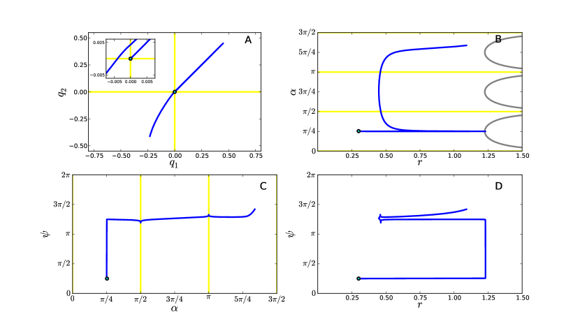
Figure 8: A near-ejection orbit starting at $(r,\alpha,\psi)=(0.3,\pi/4+10^{-2},\pi/4)$ with $h=0$. The initial conditions are transformed to physical coordinates using equations (40) and (41), then a numerical integration of the equations (5) with the potential (33) and $\epsilon=10^{-6}$ generates the orbit. Panel A): the orbit in physical coordinates, projected on the $(q_{1},q_{2})$ plane. The inset magnifies the region close to the origin (corresponding to the total collapse). Panels B), C), D): the orbit transformed back to McGehee coordinates, projected respectively on the $(r,\alpha)$, $(\alpha,\psi)$, and $(r,\psi)$ planes. For clarity, after each binary collision the orbit is extended with continuity into the adjacent domain, rather than into the fundamental one, which would introduce visually bothersome jumps in the $\psi$ coordinate. The circle shows the position of the initial condition. The yellow lines at $\alpha=0,\pi,\cdots$ correspond to binary collisions at $q_{1}=0$, those at $\alpha=\pi/2,3\pi/2,\cdots$ to binary collisions at $q_{2}=0$. The grey lines in panel B) are the points with $\hat{E}=0$.

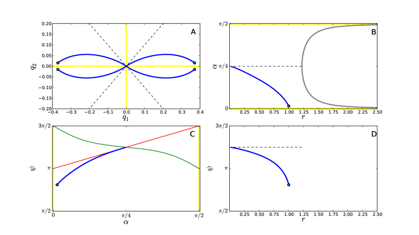
Figure 9: An orbit as close as numerically possible to one lying on the center manifold of the total collision point $(r,\alpha,\psi)=(0,\pi/4,5\pi/4)$. The orbit starts approximately at $(r,\alpha,\psi)=(1.00264534\cdots,0.04149204\cdots,2.54344846\cdots])$ with $h=0$. The dashed lines are the homothetic orbit corresponding to the heterocline $\eta_{24}$. The red and the green curve in panel C) are, respectively, the projection on the $(\alpha,\psi)$ plane of the lines of rest points $\mathscr{P}_{2}$ and $\mathscr{P}_{4}$. Details of the numerical solution and panel description as in figure 8.

Summarizing we have

Theorem 6.1

The only homothetic ejection/collision orbit from/to total collapse is that homothetic to the planar central configuration, which is bounded.

Proof.  The existence and boundedness of the ejection/collision orbit homothetic to the planar central configuration is a direct consequence of Proposition 4.4. For a hypothetical solution where the position of the vortices is at all times a homothetic transformation of the vertices of a given rectangle, then the momentum of each vortex would be parallel to the line joining the vortex and the origin. However, it is clear that only at $\alpha=\pi/4$ all the forces are balanced, therefore we exclude other solutions. $\Box$

Remark 6.2

Recalling from Sundman type estimates proven in [BaFeTe08] that, of all the points on the collision manifold, those corresponding to a homothetic ejection/collision (namely $(\alpha,\psi)=(\pi/4,\pi/4)$ and $(\alpha,\psi)=(\pi/4,5\pi/4)$) are dynamically reachable from outside the manifold, then the other rest points on the collision manifold and the heteroclinic connections between them are dynamically meaningless.

Theorem 6.3

Each solution different from the homothetic central configuration experiences a binary collision in finite time. Moreover, any solution starting arbitrarily close to the homothetic ejection solution has an orbit that may not reach the upper bound of the homothetic orbit before experiencing a binary collision.

Proof.  This is a direct consequence of the theorem 5.3. $\Box$

When the four vortices are arranged at the vertex of a rectangle with a large ratio of side lengths, then there are solutions in which the pairs of vortices undergo repeated binary collisions along the same axis. In particular, for some of these solutions the sequence of collisions initially moves away from the origin of the Cartesian axes. However, unbounded solutions are not possible, and eventually the sequence reaches a turning point and returns towards the origin. An example of this dynamical behavior is shown in figure 10. When seen in the McGehee coordinates, these are solutions advancing (up to a turning point) into the narrow funnel between the zero velocity manifolds of adjacent domains. In figure 11 we show a numerical solution where a sequence of binary collisions approaching the origin from the right undergoes a single binary collision along the $q_{2}$ axis and the continues moving leftward on the negative $q_{1}$ semi-axis, although with a markedly different amplitude. Eventually, this it will reach a turning point, and return towards the origin. Solutions that oscillate along an axis bouncing back and forth between turning points of opposite sign are not uncommon. However, we were unable to maintain the oscillations, which are aperiodic, for arbitrarily long times. Eventually the orbit spends some time winding closely around the origin at distances corresponding to values of $r$ such that $\hat{E}(h,r,\alpha)>0$ for any $\alpha$. After these complicated and chaotic-looking transients the orbit may resume its oscillations along one (not necessarily the same) axis.

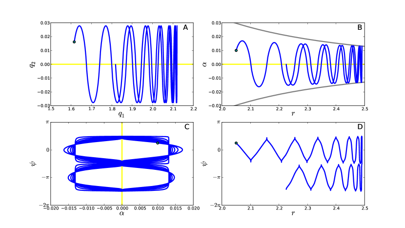
Figure 10: A sequence of binary collisions moving along the positive $q_{1}$ semi-axis with a turning point. The orbit starts at $(r,\alpha,\psi)=(2.05,0.01,\pi/4)$ with $h=0$. Details of the numerical solution and panel description as in figure 8.

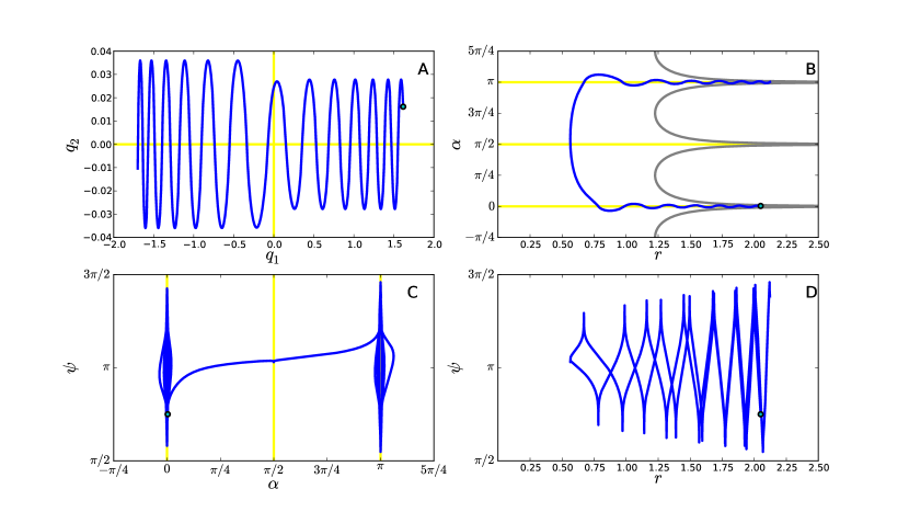
Figure 11: A sequence of binary collisions moving from the positive to the negative $q_{1}$ semi-axis. The orbit starts at $(r,\alpha,\psi)=(2.05,0.01,3\pi/4)$ with $h=0$. Details of the numerical solution and panel description as in figure 8.

We may formalize these findings as follows.

Theorem 6.4

If the initial configuration is a rectangle with large enough aspect ratio, the configuration evolves by passing through an arbitrary number of simultaneous binary collisions between the pairs of closest vortices.

Theorem 6.5

The projection of any solution in the configuration space is bounded.

Proof.  This is a direct consequence of theorem 5.2. $\Box$

Theorem 6.6

The set of initial conditions leading to total collapse or leading in an infinite amount of time to the outermost boundary region where the motion is allowed has zero Lebesgue measure.

From the physical point of view the outermost boundary region among the others depends on the total energy $h$ of the system and it is given by the hypersurface having the property that any solution of the Newton equations after reaching with zero velocity, the solution orbit falls down.

Finally, we may go back to the initial interpretation of the equations of motion (4) as steady solutions of the equations (1) for infinitely tall, nearly parallel, vortex filaments in a three-dimensional space. In that setting our time-like variable really is the arc-length parameter along the vortex filament. From this point of view an orbit of our dynamical system describes the mutual position of four steady vortex filaments at various heights. The points of intersection of the vortex filaments with an horizontal plane, and the inclination of tangent to the filaments at the intersection points are the parameters that completely determine the shape of the whole filament. In particular, some of our findings about the equivariant solutions subject to the $D_{2}$ symmetry may be recast as follows:

1. If the vortex filaments join together into a total collapse, or separate from collapse, then they do so by approaching a square configuration;

2. the distance among the vortex filaments is bounded at all heights;

3. binary collisions of the vortex are generic, that is, the set of intersection points and tangents generating non-colliding filaments has zero Lebesgue measure.

7 Further perspectives and closing remarks

Among all the solutions of a system of vortex filaments some special and very important class is represented by the so-called helicoidal solutions, namely solutions of (1) of the form.

$$\Psi(\sigma,t)=e^{i\nu t}{\bm{q}}(\sigma)$$

for some complex valued function ${\bm{q}}:\mathbb{R}\to\mathbb{C}$. In the special case in which ${\bm{q}}(\sigma)=\lambda(\sigma){\bm{\xi}}$ it is called a homographic solution and if if $\lambda(\sigma)=e^{i\nu\sigma}$ we shall refer as a relative equilibrium. We observe that, for fixed frequencies $\omega,\nu$ the function

$$\Psi(\sigma,t)=e^{i\omega\sigma}\,e^{i\nu t}{\bm{\xi}}$$

only depends on the choice of the configuration ${\bm{\xi}}$. Moreover every filament has the same shape of helicoidal type and the time evolution corresponds to a rotation equal for each vortex filament of the initial configuration. Therefore the solution $\Psi$ is periodic in $\sigma$ and constant in time.

1. An interesting question that should be addressed is to consider helicoidal solutions instead of stationary solution. In this case the dihedral potential we need to add a quadratic term. However we think that our techniques should work also in this case.

2. Of some interest in the applications is the study of a singular logarithmic type potential on a more general surface without boundary.

As already observed in the introduction this transformation was firstly introduced in Celestial Mechanics by R. McGehee in its celebrated paper [McG74]. Furthermore this technique became a milestone in order to investigate the orbital structure of the $n$-body problem in the neighborhood of total collapse. In fact it was employed in several problem giving a lot of important feature on the global dynamics of this interesting problem. However in that context, due to the fact that the potential is a homogeneous function (of degree $-1$) allow us to decouple the system in a scalar equation containing the radial part and in a system which take into account the angular part. Therefore it makes this technique more feasible for the application. In fact it is possible to study separately the angular and radial part; in this perspective it is possible to read the full behavior of the system by looking only at the angular part. All of this breakdown in our context since the potential is not homogeneous anymore.

Another important difference which makes things more involved is that the equilibrium points are not isolated (in fact they appear in family) and they do not have a hyperbolic character (and only some of them are normally hyperbolic manifolds). For instance, to the knowledge of the authors it is not known if there exists a sort of Palis Inclination Lemma in this context.

However since the differential of the potential is a homogeneous function, this still guaranteed the existence of self-similar (homothetical, homographical) motions.

As direct consequence of the energy relation, for each fixed energy level $h$ the motion is confined between the two invariant manifold ($\hat{E}=0$, $r=0$) and the hyperplanes corresponding to the simultaneously binary collision. However as already observed the region in which the motion is allowed is not compact. This is completely different for instance with the case studied by the authors in [StFo03] and in our case a priori unbounded motion can happen. However as proved above there are no unbounded orbits.

An intriguing question is to understand if this weak logarithmic singularities always prevents the existence of unbounded motions.

References

- [BaFeTe08] Barutello, Vivina; Ferrario, Davide L.; Terracini, Susanna On the singularities of generalized solutions to -body-type problems. Int. Math. Res. Not. IMRN 2008.
- [BaFuGr03] Bellettini G., Fusco G:, Gronchi G.F. Regularization of the two body problem via smoothing the potential Commun. Pure Appl. Anal., 2 n. 3 (2003) 323–353.
- [Cas05] Roberto Castelli Moti periodici di filamenti vorticosi quasi-paralleli Laurea Magistrale dissertation at University of Milano-Bicocca, 2004.
- [Cas09] Roberto Castelli On the variational approach to the one and N-centre problem with weak forces. Ph.D. dissertation at University of Milano-Bicocca, 2009.
- [CaTe] Roberto Castelli, Susanna Terracini On the regularization of the collision solutions of the one-center problem with weak forces To appear on Journal of Mathematical Analysis and Applications. http://arxiv.org/abs/0905.1579
- [DeG96] De Giorgi Ennio Conjectures concerning some evolution problems. Duke Math. J, 81, n. 2 (1996), 255–268.
- [DeVi99] Delgado, J., and Vidal, C. The tetrahedral -body problem. J. Dynam. Differential Equations 11, 4 (1999), 735–780.
- [Dev80] Devaney, R. L. Triple collision in the planar isosceles three-body problem. Invent. Math. 60, 3 (1980), 249–267.
- [Dev81] Devaney, R. L. Singularities in classical mechanical systems. In Ergodic theory and dynamical systems, I (College Park, Md., 1979–80), vol. 10 of Progr. Math. Birkhäuser Boston, Mass., 1981, pp. 211–333.
- [Fer07] Ferrario, Davide L. Transitive decomposition of symmetry groups for the -body problem. Adv. in Math. 2 (2007), 763–784.
- [FePo08] Ferrario, Davide L., Portaluri, Alessandro On the dihedral - body problem. Nonlinearity 21 (2008), 6 1307–1321.
- [Fis04] Fischer, Todd On the structure of Hyperbolic Sets Ph.D. Dissertation, Nortwestern University 2004
- [HiPuSh77] Hirsch, M. W.; Pugh, C. C.; Shub, M. Invariant manifolds. Lecture Notes in Mathematics, Vol. 583. Springer-Verlag, Berlin-New York, 1977
- [KlMaDa95] Klein, Rupert; Majda, Andrew J.; Damodaran, Kumaran Simplified equations for the interaction of nearly parallel vortex filaments. J. Fluid Mech. 288 (1995), 201–248.
- [McG74] McGehee, R. Triple collision in the collinear three-body problem. Invent. Math. 27 (1974), 191–227.
- [Moe81] Moeckel, R. Orbits of the three-body problem which pass infinitely close to triple collision. Amer. J. Math. 103, 6 (1981), 1323–1341.
- [Moe83] Moeckel, R. Orbits near triple collision in the three-body problem. Indiana Univ. Math. J. 32, 2 (1983), 221–240.
- [New01] Newton, Paul The -vortex problem. Analytical techniques. Applied Mathematical Sciences, 145. Springer-Verlag, New York, 2001.
- [Sun09] Sundman, K. F. Nouvelles recherches sur le probleme des trois corps. Acta Soc. Sci. Fenn. 35, 9 (1909).
- [StFo03] Stoica, Cristina; Font, Andreea. Global dynamics in the singular logarithmic potential. J. Phys. A , 36 (2003), 7693–7714.
- [Vid99] Vidal, C. The tetrahedral -body problem with rotation. Celestial Mech. Dynam. Astronom. 71, 1 (1998/99), 15–33.