Limitations to sharing entanglement

Abstract

We discuss limitations to sharing entanglement known as monogamy of entanglement. Our pedagogical approach commences with simple examples of limited entanglement sharing for pure three-qubit states and progresses to the more general case of mixed-state monogamy relations with multiple qudits.

I Introduction

Entanglement is one of the most important feature of quantum mechanics and arises from applying the quantum superposition principle to multiple systems Plenio and Vedral (1998); Horodecki et al. (2009). In its bipartite form, entanglement is at the heart of Bell inequality violations, which yield spacelike-separated detector correlations that exceed the degree of correlation permitted within the framework of local realism. Recently entanglement has been recognized as a key consumable resource in quantum communication, for example to teleport Bennett et al. (1993) or to perform dense coding Bennett and Wiesner (1992). Entangled states can be used by two parties to perform secure quantum key distribution Ekert (1991), and, although entangled states are not required for the Bennett-Brassard 1984 quantum key distribution protocol known as BB84 BB8 (1984), an entangled-state analysis is used to prove the security of privacy amplification for overcoming errors in establishing the key. Entanglement is essential in certain models of quantum computing such as non-deterministic gate teleportation Nielsen and Chuang (1997); Hillery et al. (2006); Mičuda et al. (2008) in cases where a deterministic gate is not feasible, and a large multi-partite state is required as the initial quantum computing “substrate” for one-way quantum computing Raussendorf and Briegel (2001).

Entanglement is a shareable resource meaning that parties in a network can transfer entanglement between themselves. These players can share entanglement by sending shares (e.g. particles) through quantum channels to each other or, alternatively, consume prior shared entanglement and employ classical communication to redistribute entanglement to other parties. Our concern here is to show that severe restrictions apply to the sharing of entanglement. These restrictions are known as monogamy relations. The terminology refers to the concept of fidelity in marriage: if two adults are committed to each other, then a third adult has no amorous access to the couple. For the case of two-level systems (quantum binary digits, or ‘qubits’ in quantum information parlance), two maximally entangled qubits share no entanglement or even classical correlations whatsoever with any other qubits (this phenomenon holds for higher level systems as well).

Monogamy of entanglement (MoE) was first proposed by Coffman, Kundu and Wootters in 2000 Coffman et al. (2000). They conjectured MoE for a network of many qubits but only succeeded in proving the quantitative monogamy relation for three qubits. The conjecture stubbornly remained unproved for several years until the proof by Osborne and Verstraete in 2006, which was a calculational tour de force Osborne and Verstraete (2006). These results show that, in a quantum network comprising $n$ parties each possessing one qubit, more entanglement shared between two parties necessarily implies less entanglement that can be shared between either of these parties with any other parties in the network. Furthermore, shared entanglement between two parties even limits the amount of classical correlation that can be shared with the other parties Koashi and Winter (2004).

Without delving into the details of entanglement measures yet, the concept of a monogamous measure of entanglement can be described as follows. Let $E_{\text{A}|\text{B}}$ denote the shared entanglement between A and B. That is to say $E_{\text{A}|\text{B}}$ measures the degree of entanglement between A and B, but of course there is more than one choice for this measure, which concerns us later. As MoE is concerned with more than two parties in a quantum network, we also consider the entanglement $E_{\text{A}|\text{C}}$ shared between A and C and the entanglement $E_{\text{A}|\text{BC}}$ shared between A and the composite system comprising B and C. In this notation, $E$ is monogamous if

$$E_{\text{A}|\text{BC}}\geq E_{\text{A}|\text{B}}+E_{\text{A}|\text{C}}$$ (1)

provided that adding $E_{\cdot|\cdot}$ is meaningful. This inequality conveys the MoE principle that the amount of entanglement shared between A and B restricts the possible amount of entanglement between A and C so that their sum does not exceed the total bipartite entanglement between A and the composite BC system.

In the seminal Coffman-Kundu-Wootters paper Coffman et al. (2000), the entanglement sharing limit of Eq. (1) was proved only for systems consisting of qubits, for which the entanglement measure $E$ can be taken to be the square of Wootters’s concurrence Wootters (1998). This squared-concurrence quantity is a measure of entanglement known also as the “tangle” whose formal definition is discussed later. The MoE relation of Eq. (1) when expressed in terms of the qubit tangle is elegant yet unsatisfying. The elegance of the expression is evident in its simplicity and in the presence of a saturable bound on the amount of entanglement that can be shared. The unsatisfying aspect of this quantum-network entanglement-sharing relation is its poor capability for direct generalization to higher dimensions. For example, suppose that the parties hold quantum $d$-ary digits, or ‘qudits’, rather than qubits. Generalizing the Wootter’s tangle from the case of qubits to the case of qudits leads to measures of entanglement that are not additive (nor superadditive). As any measure of entanglement that satisfies the monogamy relation (1) must be additive or super-additive (see Sec. V.3 for details) the generalization of the qubit monogamy relation in Coffman et al. (2000) to qudits is impossible.

A natural question therefore arises: is there a measure of entanglement satisfying Eq. (1) for all dimensions? Whereas most known measures of entanglement (like entanglement of formation Wootters (1998) or the relative entropy of entanglement Vedral et al. (1997); Vedral and Plenio (1998)) are not monogamous, there exists one measure, called the squashed entanglement, which satisfies Eq. (1) in all dimensions. The existence of such a measure indicates that MoE can be quantified, but since the squashed entanglement is extremely hard to compute even numerically (see Sec. V.3 for more details), our knowledge about the sharability of entanglement in general non-qubit quantum networks is very limited.

As MoE is an interesting fundamental property of quantum mechanics and yet is not mathematically settled for general quantum networks, our aim here is to introduce and explain MoE in a way that avoids the daunting mathematical complexity of the subject and instead builds a conceptual foundation. We commence by focusing on extremal cases of pure-state three-qubit quantum networks and progress to the general three-qubit network. Subsequent to building this foundation, we discuss multi-qubit quantum networks in a gentle way. Using these concepts we show how to bound the tangle using a dual relation to MoE, sometimes called polygamy of entanglement Gour et al. (2007); Buscemi et al. (2009); Kim (2009).

II Entanglement in a network and the concept of monogamy of entanglement

Entanglement refers to quantum correlations between two or more parties. The state shared between two parties A and B is designated $\rho_{\text{AB}}$ and called a bipartite state. Mathematically, it is a unit-trace bounded operator on the tensor-product Hilbert space

$$\mathscr{H}_{\text{A}}\otimes\mathscr{H}_{\text{B}}$$

for $\mathscr{H}_{\text{A}}$ the Hilbert space for A and $\mathscr{H}_{\text{B}}$ the Hilbert space for B. A state is ‘pure’ if and only if $\rho=\rho^{2}$; otherwise the state is ‘mixed’. A pure state can be expressed as a projector $|\psi\rangle\langle\psi|$ in Dirac notation with $|\psi\rangle\in\mathscr{H}$ so here we often refer to pure states as elements of Hilbert space $\mathscr{H}$ whereas mixed states are always elements of $\mathcal{B}(\mathscr{H})$, i.e.  bounded operators (or density matrices) acting on $\mathscr{H}$.

Entanglement is a key ingredient of many counter-intuitive quantum phenomena. Besides being of interest from a fundamental point of view, entanglement has been identified as a non-local resource for quantum information tasks. In particular, shared bipartite entanglement is a crucial resource for many quantum communication tasks such as teleportation.

Such a scenario, in which parties sharing a composite quantum system are only able to perform local operations on their share of the system, arises naturally (as systems A and B can be located far from each other) and is quite common in quantum information theory. Communicating classical information is considered to be easy. Local quantum operations assisted by classical communication is known as local operations with classical communication (LOCC), and we will use this acronym frequently.

In quantum information science, entanglement is quantified by its ability to overcome the LOCC restriction. Therefore, a bipartite state is entangled if and only if it cannot be prepared by LOCC between two parties A and B. This definition of an entangled state is consistent with our intuition that the term entanglement refers to non-local quantum correlations. That is, classical communication cannot generate quantum correlations, and local operations cannot generate non-local correlations. Therefore, LOCC cannot generate entanglement nor can it increase entanglement. For this reason entanglement must be quantified by functions that do not increase under LOCC.

States that can be prepared by LOCC (i.e. , states with zero entanglement) are called separable states and they have a particular form, as we now discuss. Consider two parties usually referred to A and B who are located far from each other, in the sense that the LOCC restriction is applied to the composite physical system they share. We ask what kind of states representing their physical system they can prepare.

Clearly A can prepare her (local) physical system in some state $\sigma_{\text{A}}$, and B can prepare his system in a state $\sigma_{\text{B}}$. In this situation, the joint composite physical system of A and B is represented by one state $\sigma_{\text{A}}\otimes\sigma_{\text{B}}$. Such a state is called a product state and it can definitely be prepared by LOCC. In fact to prepare a product state there is no need for classical communication.

Consider now a situation in which A and B can prepare their physical systems in one out of several states $\{\sigma^{(\ell)}_{\text{A}}\}$ and $\{\sigma^{(\ell)}_{\text{B}}\}$, respectively. Here the integer $\ell$ distinguishes between the different states. Consider also a protocol in which A choose to prepare the state $\sigma^{(\ell)}_{\text{A}}$ according to a fixed probability distribution $p_{\ell}$. Then, once she choose $\ell$ she communicates it (classically, for example by telephoning) to B who then prepares his system in the state $\sigma^{(\ell)}_{\text{B}}$.

At the end of this protocol the composite system of A and B is described by the product state $\rho^{(\ell)}_{\text{A}}\otimes\rho^{(\ell)}_{\text{B}}$ which occurs with probability $p_{\ell}$. If A and B ‘forget’ (or lose) the information about $\ell$, then their composite physical system is represented by a separable state $\rho_{\text{AB}}$ which is given by

$$\rho_{\text{AB}}\equiv\sum_{\ell}p_{\ell}\;\sigma^{(\ell)}_{\text{A}}\otimes\sigma^{(\ell)}_{\text{B}}.$$ (2)

Any bipartite state $\rho_{\text{AB}}$ that has the form above is called a ‘separable state’.

Separable states represent physical systems with no entanglement because they can be prepared by LOCC. A bipartite quantum state $\rho_{\text{AB}}$ that is not separable is called an entangled state. Recall that quantum states such as $\rho_{\text{AB}}$ above are square Hermitian matrices with non-negative eigenvalues that sum to one. It is therefore not straightforward to determine whether a bipartite state $\rho_{\text{AB}}$ can be written in the form (2) or not. Indeed, determining whether or not a state is entangled, and how much entanglement is inherent within the state, are hard tasks.

One reason for the difficulty is that the state $\rho$ needs to be known in order to evaluate entanglement, but the matrix representation has size $d^{2}$ for $d$ the dimension of the Hilbert space. As $d$ is exponential in the number of qubits or qudits encoding the quantum information, tomography for determining the full state is generically hard. In fact even with complete knowledge of the state, deciding whether a state is entangled or not is computationally hard. An example of a hard problem class is NP (nondeterministic polynomial), which refers to the class of computational problems whose best-known algorithms require exponential time to solve but candidate solutions are easy (polynomial time) to verify. Deciding whether a state is entangled or not is NP-hard Gurvits (2004); Gharibian (2010), meaning that the problem is known to be at least as hard as other problems believed to be in the NP class.

We do not consider this problem here, but one way that partially overcomes this problem is to introduce entanglement witnesses Horodecki et al. (1996). An entanglement witness is an Hermitian operator or an observable of a geometric nature (in the terminology of convex sets is called a supporting hyperplane Pittenger and Rubin (2002)) that distinguishes entangled states from separable ones. More precisely, for every entangled state $\rho$ there exists an Hermitian operator $W$ (the entanglement witness) such that the expectation value of $W$ with respect to $\rho$ is negative, i.e. ,

$$\text{Tr}(\rho W)<0,$$ (3)

whereas the expectation value is positive with respect to all separable states.

One problem with entanglement witnesses is that they tend to deliver only one-sided answers to the decision problem: if the expectation value is negative then the state is entangled, but if the expectation value is non-negative, whether that state is separable or entangled is not known for sure. Therefore, entanglement witnesses can be very useful in determining whether a state is entangled or separable, as long as their number is kept small.

As can be seen in Eq. (1), monogamy of entanglement is defined relative to some measure of entanglement $E$. Measures of entanglement are non-negative real valued functions on the space of density matrices (i.e. , quantum states). They are expected to satisfy certain conditions, such as having the value zero for separable states. Perhaps the most important property of measures of entanglement is their monotonicity, whereby different parties cannot increase the total average entanglement by LOCC.

Over the past decade many measures of entanglement have been introduced pertaining to entanglement theory. Many of these measures are unfortunately not additive (nor superadditive), and as we see in Sec. V.3, additivity does play a crucial role in MoE relations.

In fact there are only a few known entanglement measures that are monogamous; that is, satisfying the monogamy relation (1). The first entanglement monogamy relation was introduced by Wootters using tangle; however it only measures the entanglement of (possibly mixed) two-qubit states Wootters (1998). Therefore, in order to discuss monogamy of entanglement for higher dimensional systems such as qutrits, we need to employ other measures of entanglement later in this paper.

Whereas monogamy of entanglement is a property of multi-party quantum correlations, here focus mainly on quantifying bipartite entanglement. The main reason for this focus is that, although Inequality (1) consists of entanglement between two parts of the composite system (note that even $E_{A|BC}$ refers to entanglement between two subsystems, namely, subsystem $A$ and the composite subsystem $BC$), Inequality (1) also yields

$$E_{ABC}\equiv E_{\text{A}|\text{BC}}-E_{\text{A}|\text{B}}-E_{\text{A}|\text{C}},$$ (4)

which is not negative and can be interpreted (for $E$ Wootters’s concurrence) as genuine tripartite entanglement Coffman et al. (2000). Therefore, quantifying genuine tripartite entanglement can be obtained by quantifying bipartite entanglement among subsystems. In this interpretation the entanglement between $A$ and $BC$ comprises the entanglement between A and B, the entanglement between A and C, and the tripartite entanglement among A, B, and C.

Let us now consider a tripartite quantum network with each party holding a qubit. If a qubit is in a pure state, we can represent it with a state $\alpha|0\rangle+\beta|1\rangle$ where $\alpha$ and $\beta$ are complex numbers and the two-dimensional vectors $|0\rangle,\;|1\rangle\in\mathbb{C}^{2}$ represents the two degrees of freedom such as spin up and spin down of a spin-$\tfrac{1}{2}$ particle.

With this notation, if the overall three-qubit state is pure, we can write the most general shared quantum state as a normalized vector in $\mathbb{C}^{2}\otimes\mathbb{C}^{2}\otimes\mathbb{C}^{2}$:

$$\left|\bm{\psi}\right\rangle_{\text{ABC}}=\sum_{\epsilon_{1},\epsilon_{2},\epsilon_{3}=0}^{1}\psi_{\epsilon_{1},\epsilon_{2},\epsilon_{3}}\left|\epsilon_{1},\epsilon_{2},\epsilon_{3}\right\rangle,$$ (5)

where $\{\left|\epsilon_{1},\epsilon_{2},\epsilon_{3}\right\rangle\equiv|\epsilon_{1}\rangle\otimes|\epsilon_{2}\rangle\otimes|\epsilon_{3}\rangle\}$ is the so-called computational basis for three qubits. For example, the state $|000\rangle$ represents three up spins, $|100\rangle$ the first spin being down and remaining two spins up, and so on. The eight coefficients $\{\psi_{\epsilon_{1},\epsilon_{2},\epsilon_{3}}\}$ are complex numbers subject to the normalization constraint $\langle\bm{\psi}|\bm{\psi}\rangle=1$. Thus, the state can be expressed as a complex vector $\bm{\psi}$ in the projective eight-dimensional complex space $P(\mathbb{C}^{2})^{\otimes 3}=P\mathbb{C}^{8}$.

Suppose now that the first two qubits A and B, share a maximally entangled state

$${\left|\Psi^{\pm}\right\rangle}_{\text{AB}}=|01\rangle\pm|10\rangle$$ (6)

(known as the ‘singlet state’ for the $-$ case), and supress the state-normalization coefficient if it is clear by context. The dropped normalization coefficient in Eq. (6) is $\frac{1}{\sqrt{2}}$. Physically this state can be realized with two spin-$\frac{1}{2}$ particles, such as an electron, where each of the two parties holds a particle in the opposite spin state, and the state is antisymmetric under exchange of particles.

If A and B share a singlet, then the pure state for the composite A, B and C system must have C’s state in a simple tensor product with the AB state. If we write C’s general single-qubit state as $|\varphi\rangle\in\mathbb{C}^{2}$, then tripartite state $\left|\bm{\psi}\right\rangle_{\text{ABC}}$ in Eq. (5) must have the form ${\left|\Psi^{-}\right\rangle}_{\text{AB}}|\varphi\rangle_{\text{C}}$. Thus, A and B sharing a singlet implies that C’s state is entirely independent. This is the essence of MoE. The question is then why C’s state must be entirely independent and why qubit C cannot also be maximally entangled with A. The answer to this question emerges from the no-cloning theorem.

The no-cloning theorem is a result of quantum mechanics that forbids the creation of identical copies of an arbitrary unknown quantum state. As A and B share a maximally entangled two-qubit state, A and B have the requisite quantum resource to teleport an unknown quantum state from one to the other. As shown in Fig. 1, suppose that A and C also share a maximally entangled two-qubit state.

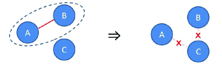
Figure 1: Two-qubit singlet state and monogamy of three-qubit systems: if subsystems A and B are in singlet state, there cannot be any entanglement shared between A and C nor B and C.

Then A can teleport an unknown quantum state to C.

This set-up can be exploited to clone an unknown quantum state as follows. A teleports the state to B and to C. Thus, this tripartite network has succeeded in copying the state: B and C each hold a copy now. However, this operation violates the no cloning theorem, which is in turn a direct consequence of the linearity of quantum mechanics Wootters and Zurek (1982). If A and B share a maximally entangled state, even if one of the two parties shares any entanglement whatsoever with the third party C, the no cloning theorem is violated. Therefore, MoE has its foundation in the linearity of quantum mechanics.

At this point we have not discussed whether Inequality (1) can saturate, and, if so, which states saturate the inequality. To address this issue, we explore genuine tripartite entanglement among all three qubits in a tripartite quantum network. Unlike the bipartite case, three qubits or more possess more than one type of entanglement. For three qubits, two quite distinct types of entanglement exist Dür et al. (2000) under stochastic LOCC (SLOCC) Dür et al. (2000), I.e., random or non-deterministic LOCC whereby only desired outputs under LOCC are retained): the W type and the Greenberger-Horne-Zeilinger (GHZ) type. The two SLOCC classes of states are defined in terms of the W state

$${\left|\text{W}\right\rangle}={\left|001\right\rangle}+{\left|010\right\rangle}+{\left|100\right\rangle}$$ (7)

and the GHZ state Greenberger et al. (1989)

$${\left|\text{GHZ}\right\rangle}={\left|000\right\rangle}+{\left|111\right\rangle}$$ (8)

with obvious normalization coefficients suppressed. W-class states and GHZ-class states are determined by whether a given three-qubit state $\left|\bm{\psi}\right\rangle_{\text{ABC}}$ can be converted to a W state or to a GHZ state, respectively, by SLOCC. Every three-qubit entangled pure state belongs to either the GHZ class or to the W class under SLOCC.

Here SLOCC is considered rather than LOCC to classify inequivalent classes of entangled states. For single copies, two pure states ${\left|\psi\right\rangle}$ and ${\left|\phi\right\rangle}$ can be obtained with certainty from each other by means of LOCC if and only if they are related by local unitaries. However, even in the simplest bipartite systems, ${\left|\psi\right\rangle}$ and ${\left|\phi\right\rangle}$ are typically not related by local unitaries, and continuous parameters are needed to label all equivalence classes. That is, one has to deal with infinitely many kinds of entanglement. In this context an alternative, simpler classification would be advisable, and one such classification is possible if we just demand that the conversion of the states is through LOCC but without imposing that it has to be achieved with certainty, that is SLOCC. In that case we can establish an equivalence relation stating that two states ${\left|\psi\right\rangle}$ and ${\left|\phi\right\rangle}$ are equivalent if the parties have a non-vanishing probability of success when trying to convert ${\left|\psi\right\rangle}$ into ${\left|\phi\right\rangle}$, and also ${\left|\phi\right\rangle}$ into ${\left|\psi\right\rangle}$.

The GHZ class is dense in the Hilbert space of three qubits, which implies that the $W$ class is of measure zero. Therefore, if a state is picked randomly (say with the Haar measure) from the space of three qubits, with unit probability it belongs to the GHZ class. The GHZ state is special in that the state is maximally entangled with respect to every bipartition (A$|$BC, AB$|$C, AC$|$B). The W state is special in that it is the only state (up to local unitary operations) that saturates the monogamy inequality (1), and also it is the only state that maximizes the average bipartite entanglement as we discuss now.

Consider the reduced density matrix for AB of the $W$ state

$$\rho_{\text{AB}}= \text{tr}_{\text{C}}{\left|\text{W}\right\rangle}_{\text{ABC}}{\left\langle\text{W}\right|}$$

$$= \frac{1}{3}{\left|00\right\rangle}_{\text{AB}}{\left\langle 00\right|}+\frac{2}{3}{\left|\Psi^{+}\right\rangle}_{\text{AB}}{\left\langle\Psi^{+}\right|},$$ (9)

which is obtained by taking the partial trace over C. Because of permutation symmetry, the states $\rho_{\text{BC}}$ and $\rho_{\text{AC}}$ are similar. The normalization of the maximally entangled state ${\left|\Psi^{+}\right\rangle}$ is needed here to ensure that the overall state (II) has unit trace and appropriate weighting in the sum. Regardless of the chosen entanglement measure $E$, it should be maximized for the state ${\left|\Psi^{+}\right\rangle}$, and, by convention, $E=1$ for maximally entangled states and $E=0$ for unentangled states. Hence, the average entanglement of the decomposition of $\rho_{\text{AB}}$ in (II) is given by

$$E\left(\rho_{\text{AB}}\right)= \frac{1}{3}E\left({\left|00\right\rangle}_{\text{AB}}{\left\langle 00\right|}\right)+\frac{2}{3}E\left({\left|\Psi^{+}\right\rangle}_{\text{AB}}{\left\langle\Psi^{+}\right|}\right)$$

$$=\frac{2}{3}.$$ (10)

Note that there are other ensemble decompositions for $\rho_{\text{AB}}$ than the one given in (II), but it can be shown Dür et al. (2000) that decomposition (II) has the minimum average entanglement. For this reason (see Sec. III), we assume $E\left(\rho_{\text{AB}}\right)=2/3$. From permutation symmetry of the $W$ state, we know that $E\left(\rho_{\text{AC}}\right)=E\left(\rho_{\text{BC}}\right)=2/3$. Thus, the the overall average bipartite entanglement of the three-qubit W state is given by

$$\frac{1}{3}\left[E\left(\rho_{\text{AB}}\right)+E\left(\rho_{\text{BC}}\right)+E\left(\rho_{\text{AC}}\right)\right]=\frac{2}{3},$$ (11)

which is the maximum possible value for any three qubit mixed state $\rho_{\text{ABC}}$ Dür et al. (2000).

The GHZ state has zero entanglement in this sense: each pair of parties has no shared entanglement after tracing out the third party. Thus, the GHZ and W states are quite different types of maximally entangled three-qubit states. The GHZ state maximizes the expected pure bipartite entanglement between any one qubit and the other two qubits, and the W state maximizes the expected mixed two-qubit bipartite entanglement after tracing out the third qubit.

Whereas three-qubit states nicely partition into the two non-overlapping W and GHZ classes, for four or more qubits systems there are uncountably many SLOCC classes, thereby making the task of classifying entanglement for more than three qubits much harder Dür et al. (2000); Gour and Wallach (2010). Further complicating matters, the existence of a state like the three-qubit GHZ state, with the property of being maximally entangled under every bipartition is unique to the three-qubits case. Although there do exist states with maximal entanglement under every bipartition for five and for six qubits, there are no such states for four qubits or more than seven qubits Gour and Wallach (2010), and the seven-qubit case remains an open question.

For the general multipartite network with a mixed state, the notion of ‘sharability’ is important in studying MoE. A bipartite state $\rho_{\text{AB}}$, which is shared by two parties A and B, is called $n$-shareable if there exists an $(n+1)$-partite quantum state $\rho_{\text{A}\textbf{B}^{(n)}}$ which is shared by one party A and $n$ parties B={B₁,…,B_n}, such that each reduced bipartite state

$$\rho_{\text{AB}_{i}}:=\text{Tr}_{\text{B}_{j}\neq\text{B}_{i}}\rho_{\text{A}\textbf{B}^{(n)}}$$ (12)

satisfies $\rho_{AB_{i}}=\rho_{\text{AB}}$ for all $i=1,2,...,n$ Masanes et al. (2006). If $\rho_{\text{AB}}$ is $n$-shareable for all $n$, then $\rho_{\text{AB}}$ is said to be $\infty$-shareable. However, the only $\infty$-shareable states are separable states Fannes et al. (1988); Raggio and Werner (1989) so bipartite entanglement cannot be shared among arbitrarily many parties whereas some mixed-state entanglement can be shared simultaneously for a finite number of parties Terhal (2004).

There is no classical counterpart to this restricted sharability of correlations as all classical probability distributions can be shared among all parties, and correlation between parties A and B (whether they are perfectly correlated or not) does not restrict A’s correlation with C. This restricted sharability in quantum physics makes MoE fundamentally different form classical physics. Throughout this article, we refer to this restricted sharability of entanglement (both pure and mixed) in multipartite systems as the monogamy of entanglement.

III Bipartite entanglement measures

Whereas MoE is a property of multipartite quantum entanglement, it is expressed in terms of bipartite measures of entanglement (1). In this section we consider choices of bipartite measures of entanglement and their suitability for MoE. In particular we consider bipartite entanglement measures for both pure and mixed states and discuss analytical evaluation of the entanglement measures for certain cases of low-dimensional quantum systems. We refer the reader to Plenio and Vedral (1998) for a comprehensive review of bipartite entanglement measures.

III.1 Entanglement of bipartite pure states

In this section we discuss how to quantify the entanglement between two parties A and B who share a pure state $\rho_{\text{AB}}=|\psi\rangle_{\text{AB}}\langle\psi|$. As entanglement cannot increase by LOCC, it must remain unchanged under reversible LOCC. An example of reversible LOCC is a local rotation or local unitary operation. To illustrate, suppose A rotates her share of the system by some angle around a particular axis. Such a rotation is reversible and is described mathematically by a unitary operator $U_{\text{A}}$.

The state of her system after rotation is $U_{\text{A}}\otimes\openone_{\text{B}}|\psi\rangle_{\text{AB}}$. As this local rotation is reversible, the entanglement of the state before the rotation must be equal to the entanglement of the state after the rotation. More generally, given two unitary matrices $U_{\text{A}}$ and $U_{\text{B}}$, the entanglement of $|\psi\rangle_{\text{AB}}$ is the same as the entanglement of $U_{\text{A}}\otimes U_{\text{B}}|\psi\rangle_{\text{AB}}$. Hence, entanglement is quantified by functions that are invariant under local unitary operations.

For pure states, this invariance under local unitary operations implies that the degree of entanglement for $\rho_{\text{AB}}=|\psi\rangle\langle\psi|$ can be understood in terms of the entropy of its reduced state either over A or over B; it does not matter which reduction as both reductions lead to the same result for entanglement. The reduced state of a bipartite state $\rho_{\text{AB}}$ is its partial trace over one of the two subsystems A or B denoted

$$\rho_{\text{A}}=\text{Tr}_{\text{B}}\rho_{\text{AB}}$$ (13)

(for a partial trace over B). The entropy of the reduced state is denoted $S(\rho_{\text{A}})$.

Many classical entropy functions are available von Neumann (1927, 1932); Rényi (1960); Tsallis (1988); Berry and Sanders (2003), which leads to a multitude of general quantum entropies $S(\rho)=\text{tr}[\rho f(\rho)]$ with function $f$ quite general. The choice of entropy function for entanglement evaluation has an impact on the resultant evaluation of entanglement of the state and therefore must be chosen judiciously.

An easy-to-calculate yet meaningful entropy is a linear function of the state ‘purity’ $\text{Tr}\rho^{2}$, namely

$$S_{\text{lin}}\left(\rho\right)=2\left(1-\text{tr}\rho^{2}\right).$$ (14)

This entropy function corresponds to choosing $f(\rho)\equiv\rho$, which is useful as the lowest-order approximation to general $S_{f}$. The purity has a maximum value of $1$ for a pure (rank-one) reduced state $\rho_{\text{A}}$ and a minimum value of $1/d$ for the completely mixed state $\rho_{\text{A}}=\frac{1}{d}\openone_{\text{A}}$ for $\openone$ the identity matrix acting on a $d$-dimensional Hilbert space $\mathscr{H}_{d}$.

As an example, the purity of the reduced one-party state obtained from the singlet state ${\left|\Psi^{-}\right\rangle}_{\text{AB}}$ (6) is

$$\rho_{\text{A}}= \text{tr}_{\text{B}}{\left|\Psi^{-}\right\rangle}_{\text{AB}}{\left\langle\Psi^{-}\right|}$$

$$= \frac{1}{2}\left({\left|0\right\rangle}_{\text{A}}{\left\langle 0\right|}+{\left|1\right\rangle}_{\text{A}}{\left\langle 1\right|}\right)$$

$$= \frac{1}{2}\openone_{\text{A}},$$ (15)

for $\openone_{A}$ the identity operator acting on subsystem A. The maximally entangled state ${\left|\Psi^{-}\right\rangle}_{\text{AB}}$ reduces to the maximally-mixed state $\frac{1}{2}I$ over either subsytem. In a sense, all the information that describes ${\left|\Psi^{-}\right\rangle}_{\text{AB}}$ is contained in entanglement or quantum correlations between subsystems A and B.

Purity clarifies the absence of entanglement in the product state ${\left|00\right\rangle}_{\text{AB}}$: the reduced state

$$\rho_{\text{A}}=\text{Tr}({\left|00\right\rangle}_{\text{AB}}{\left\langle 00\right|})={\left|0\right\rangle}_{\text{A}}{\left\langle 0\right|}$$ (16)

has a purity of one, and the same relation holds for subsystem B. Therefore, entanglement or correlation cannot exist in this bipartite state. The entropic measure $S_{\text{lin}}\left(\rho\right)$ (14) quantifies the uncertainty associated with the eigenvalue spectrum of $\rho$. In particular, the entropy vanishes if $\rho$ is a pure state, and, for a two-dimensional system (i.e.  qubit), this measure attains its maximum value for the maximally-mixed state $\openone/2$.

These examples of the singlet and product states illustrate the quantitative relation between the entanglement of a bipartite pure state and the purity of the states of subsystems. The entanglement of a bipartite pure state ${\left|\psi\right\rangle}_{\text{AB}}$ is maximal if the purity of its subsystems represented by the reduced density operator $\rho_{\text{A}}$ or $\rho_{\text{B}}$ is minimal. The pure state ${\left|\psi\right\rangle}_{\text{AB}}$ has no entanglement if $\rho_{\text{A}}$ and $\rho_{\text{B}}$ are maximally pure, i.e.  pure states. Furthermore, we also obtain an intuitive way to quantify the entanglement of a bipartite pure state by quantifying the purity of its reduced density matrices; less purity of reduced density matrices implies more entanglement between subsystems. The entanglement between subsystems A and B for a pure state ${\left|\psi\right\rangle}_{\text{AB}}$ is inversely proportional to the purity of the subsystems.

Linear entropy can be used to quantify the entanglement of a bipartite pure state. We use the tangle

$$\tau\left({\left|\psi\right\rangle}_{\text{AB}}{\left\langle\psi\right|}\right):=S_{\text{lin}}(\rho_{\text{A}}),$$ (17)

with the reduced density operator $\rho_{\text{A}}=\text{Tr}_{\text{B}}{\left|\psi\right\rangle}_{\text{AB}}{\left\langle\psi\right|}$ Wootters (1998). This measure yields $0$ for product states and $1$ for a maximally-entangled two-qubit state. Furthermore, it can be shown that this measure cannot increase on average under LOCC Vidal (2000), which is expected for a proper measure of entanglement. That is, entanglement or quantum correlations should not increase by local means. In the following subsection, we generalize this pure-state measure of entanglement to the case of mixed states. In general, mixed-state entanglement is hard to calculate, but we will see that the generalization of the tangle to mixed two qubit states can be computed analytically.

III.2 Entanglement of bipartite mixed states

In Subsec. III.1 we studied tangle for pure bipartite states. In this subsection we extend this analysis in a natural way to the case of mixed bipartite states. Any bipartite mixed state $\rho_{\text{AB}}$ is Hermitian and therefore can be written as the sum

$$\rho_{\text{AB}}=\sum_{i}p_{i}|\psi_{i}\rangle_{\text{AB}}\langle\psi_{i}|\;,$$ (18)

Intuitively the mixed state $\rho_{\text{AB}}$ is a mixture of pure states

$$\{|\psi_{i}\rangle_{\text{AB}},p_{i}\}$$ (19)

with $|\psi_{i}\rangle_{\text{AB}}$ a pure bipartite state and $p_{i}$ its probability.

This decomposition is not unique as another mixture of pure states can lead to the exact same state $\rho_{\text{AB}}$. Therefore, all decompositions $\{|\psi^{\prime}_{j}\rangle_{\text{AB}},p^{\prime}_{j}\}$ for which

$$\rho_{\text{AB}}=\sum_{j}p^{\prime}_{j}|\psi^{\prime}_{j}\rangle_{\text{AB}}\langle\psi^{\prime}_{j}|$$ (20)

are equally valid. We note that even the cardinality of different decompositions is not the same in general.

For each pure state $|\psi_{i}\rangle$ we know the tangle $\tau(|\psi_{i}\rangle\langle\psi_{i}|)$ (17). If we regard the mixed state $\rho$ as an ensemble of pure states, each with known tangle, we can characterize the tangle of the mixed state as some function of the collection of tangles of elements in the ensemble. As an example, consider the average tangle in the ensemble $\{|\psi_{i}\rangle_{\text{AB}},p_{i}\}$:

$$\sum_{i}p_{i}\tau\left({\left|\psi_{i}\right\rangle}_{\text{AB}}{\left\langle\psi_{i}\right|}\right).$$ (21)

As the decomposition of $\rho$ into ensemble of pure states is not unique, the expectation value of tangle depends on which ensemble is selected. Our concern is with forming entangled states in the least expensive way possible. The relevant expectation value of tangles is the infimum of the average entanglement over all decompositions.

Of course the question arises as to whether, for general $\rho_{\text{AB}}$, there even exists a decomposition of $\rho$ such that its average entanglement equals the infimum. The answer to this question is an emphatic yes because the set of all ensembles for $\rho$ is compact, and average tangle is a continuous function defined on the set of ensembles. Although the decomposition with the minimum average entanglement is known to exist, minimization is a NP-hard problem and hence intractable in general. Fortunately, for two-qubit mixed states, an analytical formula is known Wootters (1998).

We illustrate now how different the expectation value of the tangle can be for different ensembles by considering two extreme examples. One example has a tangle of zero and the other a tangle of one for the same state. Consider the two-qubit maximally-mixed state

$$\rho_{\text{AB}}= \frac{1}{4}\openone_{AB}$$

$$= \frac{1}{4}\Big{(}{\left|00\right\rangle}_{\text{AB}}{\left\langle 00\right|}+{\left|01\right\rangle}_{\text{AB}}{\left\langle 01\right|}$$

$$+{\left|10\right\rangle}_{\text{AB}}{\left\langle 10\right|}+{\left|11\right\rangle}_{\text{AB}}{\left\langle 11\right|}\Big{)},$$ (22)

with

$$\{{\left|00\right\rangle}_{\text{AB}},{\left|01\right\rangle}_{\text{AB}},{\left|10\right\rangle}_{\text{AB}},{\left|11\right\rangle}_{\text{AB}}\}$$ (23)

the standard orthonormal ‘computational’ basis for the two-qubit system AB.

As each pure state in the decomposition is a product state, the average tangle of the decomposition (22) is trivially zero. Expressed in the two-qubit systems Bell basis $\{{\left|\Psi^{\pm}\right\rangle},{\left|\Phi^{\pm}\right\rangle}:={\left|00\right\rangle}\pm{\left|11\right\rangle}\}$, the maximally-mixed state (22) can be written as

$$\rho_{\text{AB}}= \frac{1}{4}\openone_{AB}$$

$$= \frac{1}{4}\Big{(}{\left|\Phi^{+}\right\rangle}_{\text{AB}}{\left\langle\Phi^{+}\right|}+{\left|\Phi^{-}\right\rangle}_{\text{AB}}{\left\langle\Phi^{-}\right|}$$

$$+{\left|\Psi^{+}\right\rangle}_{\text{AB}}{\left\langle\Psi^{+}\right|}+{\left|\Psi^{-}\right\rangle}_{\text{AB}}{\left\langle\Psi^{-}\right|}\Big{)}.$$ (24)

However, each Bell state in this decomposition is a two-qubit maximally entangled state so the average tangle of this decomposition is maximal, which is markedly different from the case of Eq. (22). Thus the average tangle in Eq. (21) is not always unique for a bipartite mixed state, and average tangle strongly depends on which pure-state ensemble we choose to represent $\rho_{\text{AB}}$.

Now consider the ‘cheapest’ way to prepare the bipartite mixed state (18) by preparing an ensemble of pure states $\{p_{i},{\left|\psi_{i}\right\rangle}_{\text{AB}}\}$ with $p_{i}$ the probability of preparing ${\left|\psi_{i}\right\rangle}_{\text{AB}}$. The least amount of resources required to prepare $\rho_{\text{AB}}$ is the average tangle minimized over all distinct decompositions $\{p_{i},{\left|\psi_{i}\right\rangle}_{\text{AB}}\}$:

$$\tau\left(\rho_{\text{AB}}\right):=\min\sum_{i}p_{i}\tau\left({\left|\psi_{i}\right\rangle}_{\text{AB}}{\left\langle\psi_{i}\right|}\right).$$ (25)

Eq. (25) serves as the definition of the tangle for mixed state $\rho_{\text{AB}}$, and the procedure of minimizing over all pure-state decompositions to determine entanglement is known as the ‘convex-roof extension’.

Many entanglement measures for bipartite mixed states are based on this concept Wootters (1998); Rényi (1960); Tsallis (1988). For example, entanglement of formation of a bipartite mixed state $\rho_{\text{AB}}$ is Bennett et al. (1996)

$$E_{\text{f}}(\rho_{\text{AB}}):= \min\sum_{i}p_{i}S_{\text{vN}}\left(\rho_{\text{A}}^{i}\right),\,\rho_{\text{A}}^{i}$$

$$:= \text{tr}_{\text{B}}{\left|\psi_{i}\right\rangle}_{\text{AB}}{\left\langle\psi_{i}\right|},$$ (26)

minimized over all pure-state ensembles, where

$$S_{\text{vN}}(\rho):=-\text{tr}\rho\log\rho$$ (27)

is the von Neumann entropy of $\rho$ von Neumann (1932). As the convex-roof extension is typically hard to evaluate because minimizing over all all possible pure-state decompositions is daunting, linear entropy is preferred for qubits. This preference arises because the qubit equations are tractable and even analytically solved Wootters (1998), which is another reason why tangle, derived from linear entropy, is so prevalent.

We complete this section by presenting the formula for the tangle of two-qubit mixed states. The formula is technical and is given in terms of the ‘spin-flipped’ two-qubit mixed state

$$\tilde{\rho}_{\text{AB}}=(\sigma_{y}\otimes\sigma_{y})\rho^{*}_{AB}(\sigma_{y}\otimes\sigma_{y})$$ (28)

with $\rho_{\text{AB}}$ the actual two-qubit state, $\rho_{\text{AB}}^{*}$ its complex conjugate with respect to the standard basis and

$$\sigma_{y}:=\begin{pmatrix}0&-i\\ i&0\end{pmatrix}$$ (29)

a Pauli operator in the standard basis. Denoting by $\{\lambda_{i}\}$ the set of eigenvalues, in decreasing order, of the Hermitian operator

$$\sqrt{\sqrt{\rho_{\text{AB}}}\tilde{\rho}_{\text{AB}}\sqrt{\rho_{\text{AB}}}},$$ (30)

the tangle of $\rho_{\text{AB}}$ has then the analytical expression Wootters (1998)

$$\tau(\rho_{\text{AB}})=\left(\lambda_{1}-\lambda_{2}-\lambda_{3}-\lambda_{4}\right)^{2},$$ (31)

for

$$\lambda_{1}\geq\lambda_{2}+\lambda_{3}+\lambda_{4};$$ (32)

otherwise, $\tau(\rho_{\text{AB}})=0$.

Other analytically evaluated entanglement measures including entanglement of formation exist for two-qubit systems Kim (2010), but their analytic evaluation is actually based on that of the tangle. In other words, the tangle is the only known bipartite entanglement measure whose evaluation for two-qubit mixed states is analytical. Wootters’s detailed proof of the analytic formula is technical and not shown here Wootters (1998).

III.3 Summary

In closing this section, we have shown that various entanglement measures are possible for bipartite systems. Furthermore, entanglement of a mixed system, expressed as a function of the average entanglement of ensemble of pure states obtained via a pure-state decomposition of the mixed state, is not unique. One of the reasons for that is that the pure-state decomposition of a mixed state is not unique. For qubit systems the tangle, derived from linear entropy, is especially appealing as an entanglement measure because of its amenability to analytical evaluation. The mixed-state tangle is the average tangle for the pure-state decomposition that uniquely minimizes this function.

The tangle and the linear entropy play a key role in the next section, which explains the MoE for three-qubit systems. Although linear entropy can be extended from qubits to higher dimensions, we see in subsequent sections that extensions of monogamy relations using linear entropy for higher dimensions is problematic.

IV Monogamy of entanglement in three-qubit systems

In this section we consider a three-party system ABC with each party holding a qubit. Earlier we saw that, if any two parties hold a pure maximally entangled state, the third party cannot share any entanglement with the first two. Our argument was based on teleportation and no cloning principles. Now we show that entanglement cannot be shared but this time using the concept of entanglement measures.

If the two parties sharing composite subsystem AB hold a pure entangled state ${\left|\psi\right\rangle}_{\text{AB}}$, then the linear entropy of this state is $S_{\text{lin}}\left({\left|\psi\right\rangle}_{\text{AB}}{\left\langle\psi_{\text{AB}}\right|}\right)=0$. The tripartite state $\rho_{\text{ABC}}$ must be a product state, $\rho_{\text{ABC}}={\left|\psi\right\rangle}_{\text{AB}}{\left\langle\psi_{\text{AB}}\right|}\otimes\rho_{\text{C}}$ for AB to share a zero-entropy state. Therefore, if two parties share a pure maximally entangled state, then there cannot be any entanglement shared between AB and anyone else, hence the concept of MoE. On the other hand, if AB share an entangled state that is not maximal, A or B or both could share some entanglement with other parties, but the amount of allowed shared entanglement is bounded.

Limited sharability of entanglement between parties is quantified by monogamy-of-entanglement mathematical relations. In this section, we discuss restricted sharability of pure and mixed bipartite entanglement for just three qubits shared by three separate parties.

IV.1 From W versus GHZ interpolation to monogamy inequality of multi-qubit entanglement

In Sec. II we examined the pure three-qubit W state (7) and GHZ state (8). All three-qubit states are equivalent to one or the other of these states under SLOCC. We start this section by showing that both the W and GHZ states are maximally entangled but in distinct ways: the W state maximizes the expected two-qubit bipartite entanglement after tracing out the third qubit whereas the GHZ state maximizes the expected bipartite entanglement between one qubit and the other two qubits. We will see that a comparison between these two distinct ways to quantify the averaged tripartite entanglement leads to a monogamy inequality that can be generalized to any number of qubits/parties.

By using the tangle to quantify the bipartite entanglement between two parties, we can quantify the expected entanglement rigorously. Consider a general three-qubit pure state

$${\left|\phi\right\rangle}_{\text{ABC}}\in\mathbb{C}^{2}\otimes\mathbb{C}^{2}\otimes\mathbb{C}^{2}$$ (33)

and denote its bipartite entanglement with respect to the three possible bi-partitions by

$$\tau_{\text{A$|$BC}},\;\tau_{\text{B$|$AC}},\;\tau_{\text{C$|$AB}}.$$ (34)

For example $\tau_{\text{A$|$BC}}$ is brief notation for $\tau_{\text{A$|$BC}}\left({\left|\phi\right\rangle}_{\text{ABC}}{\left\langle\phi\right|}\right)$, which measures the tangle between qubit A and the 2-qubit system BC. With this notation we define the expectation value of the tangle, denoted here by

$$\tau_{1}\left({\left|\phi\right\rangle}_{\text{ABC}}{\left\langle\phi\right|}\right):=\frac{\tau_{\text{A$|$BC}}+\tau_{\text{B$|$AC}}+\tau_{\text{C$|$AB}}}{3}$$ (35)

with each bipartition allotted equal importance (i.e. , weight). The average tangle $\tau_{1}$ is always non negative, and, for three-qubit systems, the tangle cannot exceed unity. This maximal value is achieved by the GHZ state, i.e. ,

$$\tau_{1}\left({\left|\text{GHZ}\right\rangle}_{\text{ABC}}{\left\langle\text{GHZ}\right|}\right)=1.$$ (36)

On the other hand, we can define another averaged value for the tangle of three qubits, denoted here by $\tau_{2}$, which is based on the two-qubit tangle inherent in a three-qubit state ${\left|\phi\right\rangle}_{\text{ABC}}$; i.e.

$$\tau_{2}\left({\left|\phi\right\rangle}_{\text{ABC}}{\left\langle\phi\right|}\right):=\frac{\tau_{\text{A$|$B}}+\tau_{\text{B$|$C}}+\tau_{\text{A$|$C}}}{3},$$ (37)

where $\tau_{\text{A$|$B}}$ (and similarly $\tau_{\text{B$|$C}}$ and $\tau_{\text{A$|$C}}$) is a short notation for $\tau\left(\rho_{\text{AB}}\right)$ where $\rho_{\text{AB}}$ (and similarly $\rho_{\text{BC}}$ and $\rho_{\text{AC}}$) is the two-qubit reduced density matrix of ${\left|\phi\right\rangle}_{\text{ABC}}$ obtained after tracing out system C. For the GHZ state

$$\tau_{2}\left({\left|\text{GHZ}\right\rangle}_{\text{ABC}}{\left\langle\text{GHZ}\right|}\right)=0,$$ (38)

because every two-qubit reduced density matrix of ${\left|\text{GHZ}\right\rangle}_{\text{ABC}}$ is separable. Thus, the averaged two-qubit entanglement in ${\left|\text{GHZ}\right\rangle}_{\text{ABC}}$ is nil despite its expected entanglement with respect to every bipartition being maximal.

Classically any correlation between subsystem A and composite subsystem BC consists of the correlation of $A$ with each of B and C. If neither B nor C is correlated with $A$, then there is no correlation between A and BC. However, the GHZ state (38) provides a counter-example to this rule in the quantum case. Quantum entanglement between system A and composite system BC does not guarantee the entanglement between A and B or between A and C.

In fact the GHZ state is an extreme quantum state whose expected bipartite entanglement between one qubit and two qubits is maximal (unity) whereas its expected two-qubit entanglement inherent is minimal (nil):

$$1= \tau_{1}\left({\left|\text{GHZ}\right\rangle}_{\text{ABC}}{\left\langle\text{GHZ}\right|}\right)$$

$$> \tau_{2}\left({\left|\text{GHZ}\right\rangle}_{\text{ABC}}{\left\langle\text{GHZ}\right|}\right)$$

$$= 0.$$ (39)

Furthermore, the inequality between $\tau_{1}$ and $\tau_{2}$ (39) is always valid for any pure three-qubit state ${\left|\phi\right\rangle}_{\text{ABC}}$. For a general three-qubit state ${\left|\phi\right\rangle}_{\text{ABC}}$, each two-qubit reduced density matrix is obtained by tracing out a one-qubit subsystem. Due to the monotonicity of entanglement, discarding subsystems does not increase entanglement so

$$\tau_{\text{A$|$BC}}\geq\tau_{\text{A$|$B}},~{}\tau_{\text{B$|$CA}}\geq\tau_{\text{B$|$C}},~{}\tau_{\text{C$|$AB}}\geq\tau_{\text{C$|$A}}$$ (40)

for the two-qubit reduced density matrices $\rho_{\text{AB}}$, $\rho_{\text{BC}}$ and $\rho_{\text{AC}}$. Relations (40) imply that

$$\tau_{1}\left({\left|\phi\right\rangle}_{\text{ABC}}{\left\langle\phi\right|}\right)\geq\tau_{2}\left({\left|\phi\right\rangle}_{\text{ABC}}{\left\langle\phi\right|}\right),$$ (41)

for any three-qubit state ${\left|\phi\right\rangle}_{\text{ABC}}$. We also observe that the GHZ state assumes the largest difference between the two terms in Inequality (41).

Inequality (41) provides an upper bound for the simultaneously shared two-qubit entanglement $\tau_{2}\left({\left|\phi\right\rangle}_{\text{ABC}}{\left\langle\phi\right|}\right)$ in terms of $\tau_{1}\left({\left|\phi\right\rangle}_{\text{ABC}}{\left\langle\phi\right|}\right)$ for a three-qubit state ${\left|\phi\right\rangle}_{\text{ABC}}$. However, this inequality is never saturated by any three-qubit entangled state: its equality holds only if ${\left|\phi\right\rangle}_{\text{ABC}}$ is a three-way product state.

Although $\tau_{1}\left({\left|\phi\right\rangle}_{\text{ABC}}{\left\langle\phi\right|}\right)$ can assume an arbitrary value between $0$ and $1$, $\tau_{2}\left({\left|\phi\right\rangle}_{\text{ABC}}{\left\langle\phi\right|}\right)$ cannot equals unity. If

$$\tau_{2}\left({\left|\psi\right\rangle}_{\text{ABC}}{\left\langle\psi\right|}\right)=1,$$ (42)

this equality would imply that all two-qubit reduced density matrices $\{\rho_{\text{AB}},\rho_{\text{BC}},\rho_{\text{AC}}\}$ are maximally entangled. Such simultaneous maximal entanglement would enable A to teleport an arbitrary unknown state to B and to C simultaneously and thereby contradict the no-cloning principle of quantum mechanics Wootters and Zurek (1982).

The averaged tangle $\tau_{2}\left({\left|\phi\right\rangle}_{\text{ABC}}{\left\langle\phi\right|}\right)$ in (41) is maximized by the W state:

$$\tau_{2}\left({\left|\phi\right\rangle}_{\text{ABC}}{\left\langle\phi\right|}\right)\leq\tau_{2}\left({\left|\text{W}\right\rangle}_{\text{ABC}}{\left\langle\text{W}\right|}\right)=\frac{4}{9}\;.$$ (43)

This upper bound follows from the closed formula in Eq. (31) for the tangle between two qubits in a mixed state and reveals the mutually-exclusive nature of mixed-state monogamy in tripartite quantum systems. In three-qubit systems $ABC$, if the amount of entanglement between two parties increases, then the amount of entanglement between other parties must decrease so that the sum of all possible two-qubit entanglement does not exceed the upper bound (43).

This mutually exclusive relation for two-qubit entanglement within three-qubit systems is most prominent for states in the $W$ class under SLOCC. States in the W class have the form

$${\left|\phi\right\rangle}_{\text{ABC}}=a{\left|100\right\rangle}_{\text{ABC}}+b{\left|010\right\rangle}_{\text{ABC}}+c{\left|001\right\rangle}_{\text{ABC}}$$ (44)

with $a,~{}b,~{}c\in{\mathbb{C}}$ satisfying $|a|^{2}+|b|^{2}+|c|^{2}=1$. The ‘W state’ is a special case in which $a=b=c=1/\sqrt{3}$. For these $W$-type states, the closed formula in Eq. (31) implies that

$$\tau_{\text{A$|$BC}}=\tau_{\text{A$|$B}}+\tau_{\text{A$|$C}}.$$ (45)

That is, W-type states saturate the monogamy relation (1). Additionally, as W-type states are symmetric under permutation of the qubits, Eq. (45) also holds under any permutation of A, B, and C. Therefore, the above equality also implies that for a three-qubit W-class state ${\left|\phi\right\rangle}_{\text{ABC}}$ under SLOCC, we have

$$\tau_{1}\left({\left|\phi\right\rangle}_{\text{ABC}}{\left\langle\phi\right|}\right)=2\tau_{2}\left({\left|\phi\right\rangle}_{\text{ABC}}{\left\langle\phi\right|}\right).$$ (46)

The first characterization of MoE in three-qubit systems was introduced by extending (45) into an inequality for a general three-qubit pure state ${\left|\psi\right\rangle}_{\text{ABC}}$. Specifically Coffman-Kundu-Wootters showed that

$$\tau_{\text{A$|$BC}}\geq\tau_{\text{A$|$B}}+\tau_{\text{A$|$C}}$$ (47)

for any three-qubit state ${\left|\psi\right\rangle}_{\text{ABC}}$ Coffman et al. (2000), which is depicted in Fig. 2.

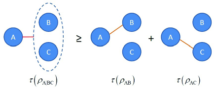
Figure 2: Characterization of bipartite entanglement shared in three-qubit systems: the Coffman-Kundu-Wootters inequality.

This Coffman-Kundu-Wootters inequality implies that Inequality (41), which never saturates for three-qubit entangled states, tightens to

$$\tau_{1}\left({\left|\psi\right\rangle}_{\text{ABC}}{\left\langle\psi\right|}\right)\geq 2\tau_{2}\left({\left|\psi\right\rangle}_{\text{ABC}}{\left\langle\psi\right|}\right)$$ (48)

for any three-qubit state ${\left|\psi\right\rangle}_{\text{ABC}}$ and is saturated for W-type states.

Inequality (47) provides a non-trivial upper bound for simultaneously shared two-qubit entanglement in three-qubit systems. Although subsystem A can be simultaneously entangled with both B and C, the sum of each entanglement cannot exceed the entanglement between A and BC. Moreover, if $\tau_{\text{A$|$BC}}=\tau_{\text{A$|$B}}=1$, meaning that A and B share maximal entanglement, Inequality (47) implies $\tau_{\text{A$|$C}}=0$. Thus there cannot be any entanglement between A and C, and Inequality (47) reduces to the singlet monogamy relation discussed in Sec. II. Note that the Coffman-Kundu-Wootters inequality is tight in a non-trivial sense because it is saturated by all three-qubit W states (44). This mutually exclusive relation of two-qubit entanglement in the Coffman-Kundu-Wootters inequality is illustrated in Fig. 2 .

We end this section generalizing the Coffman-Kundu-Wootters inequality to three-qubit mixed states and to more than three qubits. Consider a three-qubit mixed state

$$\rho_{\text{ABC}}=\sum_{i}p_{i}{\left|\psi_{i}\right\rangle}_{\text{ABC}}{\left\langle\psi_{i}\right|}.$$ (49)

Let us assume that $\{p_{i},\;{\left|\psi_{i}\right\rangle}_{\text{ABC}}\}$ is the optimal decomposition minimizing the average tangle of $\rho_{\text{ABC}}$ with respect to the bipartite cut between A and BC. In other words

$$\tau_{\text{A$|$BC}}\left(\rho_{\text{ABC}}\right)=\sum_{i}p_{i}\tau_{\text{A$|$BC}}\left({\left|\psi_{i}\right\rangle}_{\text{ABC}}{\left\langle\psi_{i}\right|}\right).$$ (50)

As each ${\left|\psi_{i}\right\rangle}_{\text{ABC}}$ in the decomposition is a three-qubit pure state, it satisfies monogamy inequality (47). Thus, for each $i$,

$$\tau_{\text{A$|$BC}}\left({\left|\psi_{i}\right\rangle}_{\text{ABC}}{\left\langle\psi_{i}\right|}\right)\geq\tau\left(\rho^{i}_{AB}\right)+\tau\left(\rho^{i}_{AC}\right),$$ (51)

with $\rho^{i}_{AB}$ and $\rho^{i}_{AC}$ the reduced density matrices of ${\left|\psi_{i}\right\rangle}_{\text{ABC}}$ onto subsystems AB and AC, respectively. Inequality (51) and Eq. (50) together yield

$$\tau_{\text{A$|$BC}}\left(\rho_{\text{ABC}}\right)\geq\tau\left(\rho_{\text{AB}}\right)+\tau\left(\rho_{\text{AC}}\right)$$ (52)

for a three-qubit mixed state $\rho_{\text{ABC}}$ and its reduced density matrices $\rho_{\text{AB}}$ and $\rho_{\text{AC}}$. Thus the Coffman-Kundu-Wootters inequality in (47) is also true for three-qubit mixed states.

Inequality (52) has been generalized for an arbitrary number of qubit-systems Osborne and Verstraete (2006). This generalization is

$$\tau\left(\rho_{\text{A}_{1}|\text{A}_{2}\cdots\text{A}_{n}}\right)\geq\tau\left(\rho_{\text{A}_{1}\text{A}_{2}}\right)+\cdots+\tau\left(\rho_{\text{A}_{1}\text{A}_{n}}\right),$$ (53)

for any $n$-party state $\rho_{\text{A}_{1}\text{A}_{2}\cdots\text{A}_{n}}$ with $\rho_{\text{A}_{1}\text{A}_{i}}$ the reduced density matrix acting on subsystems $\text{A}_{1}\text{A}_{i}$ for $i=2,\ldots,n$.

IV.2 Polygamy: dual monogamy inequality in multi-party quantum systems

In this section we discuss a concept that is dual to monogamy of entanglement. In particular we shall see that, whereas sharing entanglement is monogamous, distributing entanglement is polygamous. Consider a bipartite mixed state $\rho_{\text{AB}}$. Any mixed state can be considered to be a reduced pure state acting over a larger Hilbert space, and constructing such a pure state from the mixed state is known as a purification. Here we denote the state arising from a purification of  $\rho_{\text{AB}}$ as ${\left|\psi\right\rangle}_{\text{ABC}}$ such that $\rho_{\text{AB}}=\text{tr}_{\text{C}}({\left|\psi\right\rangle}_{\text{ABC}}{\left\langle\psi\right|})$. Party C can help to increase the entanglement of $\rho_{\text{AB}}$ by performing measurements on C’s own subsystem and then communicating the measurement results to A and B.

As an extreme example, consider the tripartite state

$${\left|\psi\right\rangle}_{\text{ABC}}\equiv{\left|\psi^{+}\right\rangle}_{\text{AB}}|0\rangle_{\text{C}}+{\left|\psi^{-}\right\rangle}_{\text{AB}}|1\rangle_{\text{C}}.$$ (54)

A simple calculation shows that the state $\rho_{\text{AB}}=\text{tr}_{\text{C}}({\left|\psi\right\rangle}_{\text{ABC}}{\left\langle\psi\right|})$ is separable, so that parties A and B do not share entanglement. However, suppose party C performs a measurement in the $|0\rangle$ and $|1\rangle$ computational basis. After such a measurement parties A and B will share the maximally entangled state ${\left|\psi^{+}\right\rangle}_{\text{AB}}$ or ${\left|\psi^{-}\right\rangle}_{\text{AB}}$ depending on the measurement outcome. With the assistance of C, parties A and B can end up with a maximally entangled state. This ability of a party who holds a purification to assist, leads to the concept of entanglement of assistance, which is defined as the maximum possible average entanglement that can be created between parties A and B with the assistance of C Laustsen et al. (2003).

A one-to-one correspondence between rank-one measurements of C and the pure-state ensembles of $\rho_{\text{AB}}$ exists Laustsen et al. (2003). This correspondence implies that the maximum average entanglement that can be created between the parties A and B is given by

$$\tau^{\text{a}}\left(\rho_{\text{AB}}\right):=\max\sum_{i}p_{i}\tau({\left|\psi_{i}\right\rangle}_{\text{AB}}{\left\langle\psi_{i}\right|}),$$ (55)

which is called the tangle of assistance, where the maximum is taken over all pure-state decompositions representing $\rho_{\text{AB}}=\sum_{i}p_{i}{\left|\psi_{i}\right\rangle}_{\text{AB}}{\left\langle\psi_{i}\right|}$.

The tangle of assistance is dual to the tangle (25) with this duality mathematically clear because the tangle of assistance is a maximum whereas the tangle is a minimum over all pure-state ensembles realizing $\rho_{\text{AB}}$. Furthermore, $\tau\left(\rho_{\text{AB}}\right)$ represents the minimum entanglement needed to create $\rho_{\text{AB}}$ (formation) whereas $\tau^{\text{a}}\left(\rho_{\text{AB}}\right)$ is the maximum amount of averaged entanglement attainable between A and B with the assistance of C. Thus, the mathematical duality between the tangle and the tangle of assistance for bipartite mixed states has physical meaning.

Whereas monogamy inequalities (53) provide an upper bound for the restricted sharability of multi-party entanglement, this same bound serves as a lower bound for the distribution of entanglement of assistance in multi-party quantum systems. In multi-qubit systems, entanglement of assistance is described mathematically as a dual inequality to (53), namely Gour et al. (2007)

$$\tau\left(\rho_{\text{A}_{1}|\text{A}_{2}\cdots\text{A}_{n}}\right)\leq\tau^{\text{a}}\left(\rho_{\text{A}_{1}\text{A}_{2}}\right)+\cdots+\tau^{\text{a}}\left(\rho_{\text{A}_{1}\text{A}_{n}}\right).$$ (56)

Inequality (56) is also called the polygamy of entanglement for multi-qubit systems.

Recently a general polygamy-of-entanglement inequality was proposed for three-party quantum systems with an arbitrary number of Hilbert-space dimensions using the von Neumann entropy Buscemi et al. (2009). In particular, for any tripartite pure state $|\psi\rangle_{\text{ABC}}$ in any number of dimensions,

$$E_{\text{A}|\text{BC}}\equiv S_{\text{vN}}(\rho_{\text{A}})\leq E^{\text{a}}(\rho_{\text{AB}})+E^{\text{a}}(\rho_{\text{AC}})$$ (57)

holds for $E^{\text{a}}$ the entanglement of assistance that is dual to the entanglement of formation Thus, for a tripartite pure state of arbitrary dimension, there exists a polygamy-of-entanglement relation in terms of entropy of entanglement (i.e.  $E_{\text{A}|\text{BC}}$) and entanglement of assistance.

Inequality (57) is the first known result for the polygamous (or dually monogamous) property of distribution of entanglement in multipartite higher dimensional quantum systems other than qubits. In addition, a tight upper bound on the polygamy-of-entanglement inequality has been proposed for an arbitrary-dimensional multi-party quantum systems Kim (2009). Recently, a general polygamy inequality of entanglement in a multi-party quantum system of arbitrary dimensions has been established in terms of entanglement of assistance Kim (2012).

V Monogamy of entanglement in higher-dimensional quantum systems

V.1 Entanglement for higher-dimensional systems

Generalization of monogamy of entanglement from the multi-qubit case to the multi-qudit case is complicated by the wealth of possible entanglement measures and the specifics drawbacks that each such measure entails. For pure bipartite states, these measures are constructed from Rényi-$\alpha$ and Tsallis-$q$ entropies (for appropriate values of $\alpha$ and $q$) Rényi (1960); Tsallis (1988).

For any quantum state $\rho$, the quantum Rényi entropy of order $\alpha$ (or Rényi-$\alpha$ entropy) is

$$S_{\alpha}(\rho):=\frac{1}{1-\alpha}\log\text{tr}\rho^{\alpha},$$ (58)

for any $\alpha>0$ and $\alpha\neq 1$. Similarly, the Tsallis-$q$ entropy of a quantum state $\rho$ is defined as

$$T_{q}(\rho):=\frac{1}{q-1}\left(1-\text{tr}\rho^{q}\right),$$ (59)

for any $q>0$ and $q\neq 1$. In the limitimg case where $\alpha\rightarrow 1$ and $q\rightarrow 1$, Rényi-$\alpha$ and Tsallis-$q$ entropies converge to the von Neumann entropy respectively, that is, Rényi-$\alpha$ and Tsallis-$q$ entropies are one-parameter generalizations of von Neumann entropy. As for the tangle whose derivation is based on the linear entropy, Rényi-$\alpha$ and Tsallis-$q$ entropies also lead us to various classes of entanglement measure for bipartite pure states, as well as the extended to mixed states via the convex-roof extension.

Analytic evaluations of these entropy-based entanglement measures for a two-qubit state $\rho_{\text{AB}}$ are based on the existence of a pure-state decomposition of $\rho_{\text{AB}}$ that realizes simultaneously the minimum average entanglement for all these entanglement measures. If the decomposition $\rho_{\text{AB}}=\sum_{i}p_{i}{\left|\psi_{i}\right\rangle}_{\text{AB}}{\left\langle\psi_{i}\right|}$ realizes the minimum average tangle such that

$$\tau\left(\rho_{\text{AB}}\right)=\sum_{i}p_{i}\tau\left({\left|\psi_{i}\right\rangle}_{\text{AB}}{\left\langle\psi_{i}\right|}\right),$$ (60)

then it also realizes the minimum average entanglement for other entropy-based entanglement measures. Moreover, these minimum values are monotonically related to each other by a continuous function Kim (2010); Kim and Sanders (2010). In other words the analytic evaluation of these measures are directly derived from that of the tangle and thus are all equivalent to each other because they can be obtained from the two-qubit tangle via a continuous function. In this sense, we observe that the tangle is the only known bipartite entanglement measure so far whose analytic evaluation is tractable in two-qubit systems.

V.2 Generalization of the Coffman-Kundu-Wootters inequality

Now we consider a possible generalization of the Coffman-Kundu-Wootters inequality into higher-dimensional quantum systems. As the tangle (25) is well-defined for bipartite quantum states of arbitrary dimension, we may expect the validity of the Coffman-Kundu-Wootters inequality itself in higher dimensions. However, there exist counter-examples that violate the Coffman-Kundu-Wootters inequality for tripartite quantum systems where any single subsystem has more than two dimensions Ou (2007); Kim and Sanders (2008).

We must conclude that the Coffman-Kundu-Wootters inequality only holds in terms of two-qubit tangles for multi-qubit systems. Even a tiny extension for any subsystem leads to a violation. For the generalization of the Coffman-Kundu-Wootters inequality to higher dimensional quantum systems, we thus need to consider other possible entanglement measures.

V.3 Squashed entanglement: an additive and monogamous entanglement measure

In this subsection we elaborate on a measure of entanglement that is monogamous, i.e., satisfies Eq. (1) for all dimensions. The existence of such a measure is important as it shows that entanglement is truly monogamous in all dimensions. In order to understand the significance of the new measure, we first discuss the intimate relationship between monogamy of entanglement in higher dimensions and another desired property of entanglement: additivity under tensor products.

An additive entanglement measure $E$ satisfies the property

$$E\left(\rho_{\text{A}_{1}\text{B}_{1}}\otimes\sigma_{\text{A}_{2}\text{B}_{2}}\right)=E\left(\rho_{\text{A}_{1}\text{B}_{1}}\right)+E\left(\sigma_{\text{A}_{2}\text{B}_{2}}\right)$$ (61)

for any bipartite state $\rho_{\text{A}_{1}\text{B}_{1}}$ and $\sigma_{\text{A}_{2}\text{B}_{2}}$. Additivity is a desirable entanglement-measure property in connection with an operational interpretation as an interconversion rate for a quantum information processing task. In such cases, the rate of the quantum information processing task is given by the regularized version of some entanglement measure, namely,

$$R=\lim_{n\to\infty}\frac{E\left(\rho_{\text{AB}}^{\otimes n}\right)}{n}\;,$$ (62)

with $E$ an entanglement measure.

If $E$ is additive, then the simple relation $R=E$ holds. Otherwise, $R$ is difficult to calculate. For example, the entanglement cost, which quantifies the rate at which many Einstein-Podolsky-Rosen pairs can be converted to many copies of a bipartite mixed state $\rho_{\text{AB}}$ by LOCC, is given in terms of the regularized version of the entanglement of formation of $\rho_{\text{AB}}$. Recently, Hastings discovered that the entanglement of formation is not additive Hastings (2009), which makes calcuatling the entanglement cost difficult.

In higher dimensions, monogamy inequalities lead to additivity or strong superadditivity of entanglement measures $E$. A strongly-superadditive entanglement measure $E$ satisfies the property

$$E\left(\rho_{\text{A}_{1}\text{A}_{2}|\text{B}_{1}\text{B}_{2}}\right)\geq E\left(\rho_{\text{A}_{1}\text{B}_{1}}\right)+E\left(\rho_{\text{A}_{2}\text{B}_{2}}\right)$$ (63)

for a four-party state $\rho_{\text{A}_{1}\text{A}_{2}\text{B}_{1}\text{B}_{2}}$.

To illustrate this requirement of strong superadditivity, first consider the two subsystems $\text{A}_{1}\text{A}_{2}$ of the four-party state $\rho_{\text{A}_{1}\text{A}_{2}\text{B}_{1}\text{B}_{2}}$ treated as a single party. Monogamy implies that

$$E\left(\rho_{\text{A}_{1}\text{A}_{2}|\text{B}_{1}\text{B}_{2}}\right)\geq E\left(\rho_{\text{A}_{1}\text{A}_{2}|\text{B}_{1}}\right)+E\left(\rho_{\text{A}_{1}\text{A}_{2}|\text{B}_{2}}\right)$$

$$\geq E\left(\rho_{\text{A}_{1}\text{B}_{1}}\right)+E\left(\rho_{\text{A}_{2}\text{B}_{2}}\right),$$ (64)

which is strongly superadditive for $E$.

Only two entanglement measures are known to be additive: squashed entanglement Christandl and Winter (2004) and logarithmic negativity Źyczkowski et al. (1998); Vidal and Werner (2002). Squashed entanglement is especially appealing because it is also monogamous for quantum systems of arbitrary dimension. For the state ‘extension’

$$\text{ext}\rho_{\text{AB}}:=\left\{\rho_{\text{ABE}};\text{tr}_{\text{E}}\rho_{\text{ABE}}=\rho_{\text{AB}}\right\}$$ (65)

being the set of all ABE mixed states in any dimension that are compatible with the joint AB state under a partial trace, the squashed entanglement for such a bipartite state $\rho_{\text{AB}}$ is

$$E_{\text{sq}}\left(\rho_{\text{AB}}\right):=\frac{\inf_{\rho_{\text{ABE}}\in\text{ext}\rho_{\text{AB}}}\left\{I(A;B|E)\right\}}{2}$$ (66)

with $I(A;B|E)$ the quantum conditional mutual information of $\rho_{\text{ABE}}$ Cerf and Adami (1997), namely,

$$I(A;B|E):= S_{\text{vN}}(\rho_{\text{AE}})+S_{\text{vN}}(\rho_{\text{BE}})$$

$$-S_{\text{vN}}(\rho_{\text{ABE}})-S_{\text{vN}}(\rho_{\text{E}}).$$ (67)

The relationship between mutual information and tripartite conditional mutual information is depicted in Fig. 3.

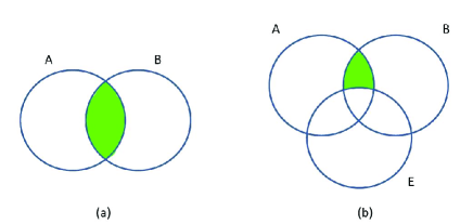
Figure 3: Venn diagrams of (a) the mutual information $I(A;B)$ and (b) the conditional mutual information $I(A;B|E)$.

For a bipartite pure state ${\left|\psi\right\rangle}_{\text{AB}}$, any possible extension $\rho_{\text{ABC}}$ such that

$$\text{tr}_{\text{C}}\rho_{\text{ABC}}={\left|\psi\right\rangle}_{\text{AB}}{\left\langle\psi\right|}$$ (68)

must be a product state

$${\left|\psi\right\rangle}_{\text{AB}}{\left\langle\psi\right|}\otimes\rho_{\text{C}}$$ (69)

for some $\rho_{\text{C}}$ of subsystem C. Thus $I(A;B|E)/2$ in Def. (66) coincides with $S_{\text{vN}}(\rho_{\text{A}})$ for any pure state ${\left|\psi\right\rangle}_{\text{AB}}$ with reduced density matrix $\rho_{\text{A}}$.

Squashed entanglement is an entanglement measure based on the entropy of subsystems for bipartite pure states, but its extension to mixed states is not achieved through the convex-roof extension. Instead squashed entanglement has appealing entanglement properties such as being an entanglement monotone, being a lower bound on entanglement of formation and being an upper bound on distillable entanglement Bennett et al. (1996); Christandl and Winter (2004).

To obtain the monogamy relation for squashed entanglement, consider a three-party state $\rho_{\text{ABC}}$ and its extension $\rho_{\text{ABCE}}$. The chain rule for quantum conditional mutual information implies that

$$I(A;BC|E)=I(A;B|E)+I(A;C|BE).$$ (70)

Minimizing $I(A;B|E)$ and $I(A;C|BE)$ over all possible E and BE, respectively, yields $E_{\text{sq}}\left(\rho_{\text{AB}}\right)$ and $E_{\text{sq}}\left(\rho_{\text{AC}}\right)$; therefore,

$$E_{\text{sq}}\left(\rho_{\text{A$|$BC}}\right)\geq E_{\text{sq}}\left(\rho_{\text{AB}}\right)+E_{\text{sq}}\left(\rho_{\text{AC}}\right).$$ (71)

Thus, squashed entanglement shows the monogamy inequality of entanglement for any tripartite state $\rho_{\text{ABC}}$. However, although squashed entanglement has beautiful properties including monogamy and being zero if and only if the state is separable Brandao et al. (2011), the difficulty of evaluating squashed entanglement makes it problematic to use in practice. Per definition, we need to consider all possible extensions $\rho_{\text{ABE}}$ of $\rho_{\text{AB}}$ without even a restriction on the dimension of subsystem E.

VI Conclusion

Beginning with a gentle introduction to entanglement and monogamy of entanglement for simple cases, we constructed mathematical monogamy relations. Rigour has been sacrificed in favour of developing an intuitive understanding of the limits to sharing entanglement and consequent limitations to sharing classical correlations as well. We have provided references so that the reader can follow up with technical material to master the rigour in this field.

In addition to establishing the foundations, we have highlighted various approaches to treating monogamy of entanglement as well as key challenges in the field. Although monogamy of entanglement and its dual polygamy relations have been studied for more than a decade, exciting problems remain open concerning limits to sharing multi-qudit entanglement. These limits could have ramifications for studying entanglement sharing capabilities of quantum networks and for assessing security strengths and weaknesses of quantum networks.

At a fundamental level, our understanding of monogamy and polygamy of entanglement is predicated on choices of entanglement measures, and development of appropriate entanglement measures is an exciting field in its own right. Furthermore choices of entanglement measures are restricted by monogamy principles: as discussed in this article, the monogamy principle forces an entanglement measure to be additive or superadditive so monogamy cannot be ignored in studies of entanglement measures.

References

- Plenio and Vedral (1998) M. B. Plenio and V. Vedral, Cont. Phys. 39, 431 (1998).
- Horodecki et al. (2009) R. Horodecki, P. Horodecki, M. Horodecki, and K. Horodecki, Rev. Mod. Phys. 81, 865 (2009).
- Bennett et al. (1993) C. H. Bennett, G. Brassard, C. Crépeau, R. Jozsa, A. Peres, and W. K. Wootters, Phys. Rev. Lett. 70, 1895 (1993).
- Bennett and Wiesner (1992) C. H. Bennett and S. J. Wiesner, Phys. Rev. Lett. 69, 2881 (1992).
- Ekert (1991) A. Ekert, Phys. Rev. Lett. 67, 661 (1991).
- BB8 (1984) Quantum cryptography: public key distribution and coin tossing (IEEE Press, New York, 1984).
- Nielsen and Chuang (1997) M. A. Nielsen and I. L. Chuang, Phys. Rev. Lett. 79, 321 (1997).
- Hillery et al. (2006) M. Hillery, M. Ziman, and V. Bužek, Phys. Rev. A 73, 022345 (2006).
- Mičuda et al. (2008) M. Mičuda, M. Ježek, M. Dušek, and J. Fiurášek, Phys. Rev. A 78, 062311 (2008).
- Raussendorf and Briegel (2001) R. Raussendorf and H. J. Briegel, Phys. Rev. Lett. 86, 5188 (2001).
- Coffman et al. (2000) V. Coffman, J. Kundu, and W. K. Wootters, Phys. Rev. A 61, 052306 (2000).
- Osborne and Verstraete (2006) T. Osborne and F. Verstraete, Phys. Rev. Lett. 96, 220503 (2006).
- Koashi and Winter (2004) M. Koashi and A. Winter, Phys. Rev. A 69, 022309 (2004).
- Wootters (1998) W. K. Wootters, Phys. Rev. Lett. 80, 2245 (1998).
- Vedral et al. (1997) V. Vedral, M. B. Plenio, M. Rippin, and P. L. Knight, Phys. Rev. Lett. 78, 2275 (1997).
- Vedral and Plenio (1998) V. Vedral and M. B. Plenio, Phys. Rev. A 57, 1619 (1998).
- Gour et al. (2007) G. Gour, S. Bandyopadhay, and B. C. Sanders, J. Math. Phys. 48, 012108 (2007).
- Buscemi et al. (2009) F. Buscemi, G. Gour, and J. Kim, Phys. Rev. A 80, 012324 (2009).
- Kim (2009) J. Kim, Phys. Rev. A 80, 022302 (2009).
- Gurvits (2004) L. Gurvits, J. Comp. Sys. Sci. 69, 448 (2004).
- Gharibian (2010) S. Gharibian, Quant. Inf. Comp. 10, 343 (2010).
- Horodecki et al. (1996) M. Horodecki, P. Horodecki, and R. Horodecki, Phys. Lett. A 223, 1 (1996).
- Pittenger and Rubin (2002) A. O. Pittenger and M. H. Rubin, Lin. Alg. Appl. 346, 47 (2002).
- Wootters and Zurek (1982) W. K. Wootters and W. H. Zurek, Nature (Lond.) 299, 802 (1982).
- Dür et al. (2000) W. Dür, G. Vidal, and J. I. Cirac, Phys. Rev. A 62, 062314 (2000).
- Greenberger et al. (1989) D. M. Greenberger, M. A. Horne, and A. Zeilinger, in Bell’s Theorem, Quantum Theory, and Conceptions of the Universe, edited by M. C. Kafatos (Kluwer Academic, Dordrecht, 1989), vol. 37 of Fundamental Theories of Physics, pp. 69–72.
- Gour and Wallach (2010) G. Gour and N. R. Wallach, J. Math. Phys. 55, 112201 (2010).
- Masanes et al. (2006) L. Masanes, A. Acin, and N. Gisin, Phys. Rev. A 73, 012112 (2006).
- Fannes et al. (1988) M. Fannes, J. T. Lewis, and A. Verbeure, Lett. Math. Phys. 15, 255 (1988).
- Raggio and Werner (1989) G. Raggio and R. F. Werner, Helv. Phys. Acta 62, 980 (1989).
- Terhal (2004) B. M. Terhal, IBM J. Research and Development 48, 71 (2004).
- von Neumann (1927) J. von Neumann, Gött. Nach. 1, 273 (1927).
- von Neumann (1932) J. von Neumann (Springer, Berlin, 1932).
- Rényi (1960) A. Rényi, Proceedings of the Fourth Berkeley Symposium on Mathematics, Statistics and Probability (University of California Press, Berkeley, 1960) 1, 547 (1960).
- Tsallis (1988) C. Tsallis, J. Stat. Phys. 52, 479 (1988).
- Berry and Sanders (2003) D. W. Berry and B. C. Sanders, J. Phys. A: Math. Gen. 36, 12255 (2003).
- Vidal (2000) G. Vidal, J. Mod. Opt. 47, 355 (2000).
- Bennett et al. (1996) C. H. Bennett, D. P. DiVincenzo, J. A. Smolin, and W. K. Wootters, Phys. Rev. A 54, 3824 (1996).
- Kim (2010) J. Kim, Phys. Rev. A 81, 062328 (2010).
- Laustsen et al. (2003) T. Laustsen, F. Verstraete, and S. J. van Enk, Quantum Inf. Comput. 3, 64 (2003).
- Kim (2012) J. Kim, Phys. Rev. A 85, 062302 (2012).
- Kim and Sanders (2010) J. S. Kim and B. C. Sanders, J. Phys. A 43, 445305 (2010).
- Ou (2007) Y. Ou, Phys. Rev. A 75, 034305 (2007).
- Kim and Sanders (2008) J. S. Kim and B. C. Sanders, J. Phys. A 75, 495301 (2008).
- Hastings (2009) M. B. Hastings, Nature Phys. 5, 255 (2009).
- Christandl and Winter (2004) M. Christandl and A. Winter, J. Math. Phys. 45, 829 (2004).
- Źyczkowski et al. (1998) K. Źyczkowski, P. Horodecki, A. Sanpera, and M. Lewenstein, Phys. Rev. A 58, 883 (1998).
- Vidal and Werner (2002) G. Vidal and R. Werner, Phys. Rev. A 65, 032314 (2002).
- Cerf and Adami (1997) N. J. Cerf and C. Adami, Phys. Rev. Lett. 79, 5194 (1997).
- Brandao et al. (2011) F. G. S. L. Brandao, M. Christandl, and J. Yard, Comm. Math. Phys. 306, 805 (2011).