Geometrical properties of Potts model during the coarsening regime

Abstract

We study the dynamic evolution of geometric structures in a poly-degenerate system represented by a $q$-state Potts model with non-conserved order parameter that is quenched from its disordered into its ordered phase. The numerical results obtained with Monte Carlo simulations show a strong relation between the statistical properties of hull perimeters in the initial state and during coarsening: the statistics and morphology of the structures that are larger than the averaged ones are those of the initial state while the ones of small structures are determined by the curvature driven dynamic process. We link the hull properties to the ones of the areas they enclose. We analyze the linear von-Neumann–Mullins law, both for individual domains and on the average, concluding that its validity, for the later case, is limited to domains with number of sides around 6, while presenting stronger violations in the former case.

I Introduction

After a rapid quench across a phase transition, two or more equilibrium states may compete for the growth of local order; this reflects in the out of equilibrium evolution observed in many different macroscopic systems once they reach the dynamic scaling regime Bray (2002); Puri (2004); Cugliandolo (2010); Corberi et al. (2011). In these systems, the properties of macroscopic observables, such as correlation functions and linear responses, can still be described in relatively simple terms by resorting to the dynamic scaling hypothesis. This hypothesis states that averaged macroscopic observables depend upon time only through a monotonically growing, time-dependent characteristic length, $R(t)$. This length, whose growth law depends on the case under consideration, characterizes the average linear size of equilibrated patches at each instant $t$. For example, after being cooled below their critical temperature magnetic systems form domains in which spins are strongly correlated and the magnetization is uniform. More precisely, on a lattice, a (geometric) domain is defined as the ensemble of nearest neighbor sites whose spins are aligned. Each of these domains has a hull or external border, whose length is the number of external sites that are first neighbors of the chosen domain Stauffer and Aharony (1994) and that, in the continuum limit, is referred as the perimeter. Figure 1 shows a sketch that illustrates, on a square lattice, this and other related definitions.

Systems as diverse as soap froths Glazier et al. (1990); Thomas et al. (2006); Weaire and Rivier (2009), cellular tissues and other natural tilings Mombach et al. (1990); Hočevar et al. (2010), magnetic grains or polycrystalline structures Babcock et al. (1990); Fradkov and Udler (1994); Jagla (2004); Kurtz and Carpay (1980a, b), type-I superconductors Prozorov et al. (2008), etc. are, in a statistical sense, geometrically similar. Their overall morphology and growth properties are well described by simple spin models with multiple ground states. An example is the ferromagnetic Potts model Wu (1982) whose variables are spins that take $q$ possible values and interact with their nearest neighbors. The coupling exchanges are taken to be isotropic and homogeneous, i.e. independent of the spin variables and lattice orientation, favoring spin alignment at low enough temperature and, therefore, the existence of $q$ degenerate equilibrium states below the phase transition. The critical temperature of the bidimensional model on the square lattice is known for all values of $q$, $k_{\scriptscriptstyle\rm B}T_{c}=2J/\ln(1+\sqrt{q})$, but the nature of the transition depends on $q$, being continuous and second-order for $q\leq 4$ while discontinuous for $q>4$. When submitted to a sudden quench from the high to the low temperature phase, and let subsequently evolve with stochastic non-conserved order parameter (the magnetization) dynamics, the system tends to organize in progressively larger ordered structures of each equilibrium state Vinals and Grant (1987); Grest et al. (1988); de Oliveira et al. (2004); de Berganza et al. (2007); Loureiro et al. (2010). One of the most common applications of this model is to crystal grain growth, where each spin configuration represents a different grain orientation and for $q\to\infty$ the continuum limit is realized Anderson et al. (1984); Srolovitz et al. (1984).

The simple presence of domains implies the existence of topological defects, in this case, the interfaces. When the final quench temperature is not too close to zero (to avoid pinning effects when $q>2$) and much lower than the critical temperature (so that the starting ordering process does not occur by nucleation when the transition is of first order) Ferrero and Cannas (2007); Loscar et al. (2009), at sufficiently long times the walls around large domains tend to be flat and the evolution (with non-conserved order parameter) is driven by their curvature. Indeed, the surface tension implies a force per unit area that is proportional to the local mean curvature, $\kappa$, acting on each point on the wall. This force is responsible for the motion of the interfaces. The field theoretical description (à la time-dependent Ginzburg- Landau equation) in the continuum leads to the Allen-Cahn equation for the local velocity, ${\vec{v}}=-(\lambda_{q}/2\pi)\kappa{\vec{n}_{s}}$, where $\lambda_{q}$ is a temperature and $q$-dependent dimensional constant related to the surface tension and mobility of a domain wall and $\vec{n}_{s}$ is a unit vector normal to the surface Allen and Cahn (1979). The sign indicates that the velocity points in the direction that tends to reduce the local curvature. Thermal effects play a minor role, affecting only the constant $\lambda_{q}$. The time-dependence of the area contained within any finite interface can be deduced by integrating the velocity around the hull, i.e. the external interface. This calculation is specially simple in $d=2$ since one can use the Gauss-Bonnet theorem to find a close expression for the area rate of change, that can be written in the following compact form:

$$\frac{dA}{dt}=\oint{\vec{v}}\wedge d{\vec{l}}=\frac{\lambda_{q}}{5}\left(n-6\right)\;\;\mbox{if}\;\;\;q\geq 2\;,$$ (1)

where $n$ is the number of sides of the external interface, each side being the border between the chosen area $A$ and one of its neighboring domains. We redefined $\lambda_{q}$ for convenience. While all non-percolating hull-enclosed areas of a system with $q=2$ states have only one side, for $q>2$ hull-enclosed areas with more than one side can exist and $n$ can be larger than one. In the latter case, the equation yields the von Neumann-Mullins law for the area $A$ of an $n$-sided hull-enclosed area von Neumann (1952); Mullins (1956). As a result, this area can grow, shrink or remain constant depending upon the number of sides being larger than, smaller than or equal to 6, respectively. Moreover, in the course of the evolution, the number of sides that a given external interface has can change, so that the equation ruling the area evolution changes through the time dependence in $n$, a function that one cannot characterize in full detail. It is also clear that for $q>2$ areas do not evolve independently of each other, as occurs for $q=2$, as $n$ is a quantity that also affects the behavior of the neighboring areas.

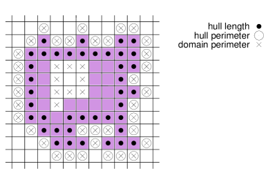
Figure 1: (Color online.) Illustration of various interfacial length definitions on the square lattice. The colored sites are all occupied by the same spin species while spins on white squares are in a different state. The hull length (solid circles) is the external border of the domain. The hull perimeter (open circles) contains only the external nearest neighbors of the domain (not the internal ones). The domain perimeter (crosses) is the ensemble of nearest neighbors of the domain and includes the internal ones as well. The measurements presented here are for the hull perimeter only.

For $q=2$, i.e. the bi-dimensional Ising model, the time-dependence of a given hull-enclosed area can be easily determined from the integration of Eq. (1) since $n(t)=1$ for all areas and these evolve independently. The number of hulls with enclosed area $A$ per unit system area ($A\gg A_{0}$, where $A_{0}$ is a small area cut-off) in the interval $(A,A+dA)$ at time $t$ is related to the distribution at the initial time $t_{0}$ through, $n_{h}(A,t)=n_{h}\left[A+\lambda_{h}(t-t_{0}),t_{0}\right]$. The two natural choices for the initial states are equilibrium at $T_{0}=T_{c}$ or $T_{0}\to\infty$ (all high temperature initial conditions become equivalent to the latter). In the former case the distribution $n_{h}$ is known analytically and in the latter it is very close to the one of critical percolation that is also known exactly Cardy and Ziff (2003). Therefore the dynamic distributions are known as well Arenzon et al. (2007); Sicilia et al. (2007). More precisely, the equilibrium critical Ising hull-enclosed area distribution is $n_{h}(A,0)=c_{h}/A^{2}$ with $c_{h}=1/(8\pi\sqrt{3})$ and one finds

$$n_{h}(A,t)=\frac{c_{h}}{[A+R^{2}(t)]^{2}}\;,$$ (2)

for $t\gg t_{0}$. Note that this expression exhibits the scaling form, $n_{h}(A,t)=t^{-2}f(A/t)$ since the characteristic length scales as $t^{1/2}$. For a quench from infinite temperature one observes that the distribution takes the critical form of random percolation in a few time steps Arenzon et al. (2007); Sicilia et al. (2007), even though the initial fraction of $+1$ (or, equivalently, $-1$) spins, 50%, is smaller than the critical density of random percolation on a square lattice, $\rho_{c}\sim 0.59$. This feature was also exploited in Barros et al. (2009) to explain the existence of percolating blocked asymptotic states in the zero-temperature dynamics of this model.

Unlike in the $q=2$ case, $n_{h}(A,t)$ is not analytically known for $q>2$. To start with, there is no simple relation between the area distribution at time $t$ and the one at the initial time $t_{0}$ and, moreover, we expect the distribution to get scrambled in a non-trivial way during the coarsening process. Thus, in a previous work Loureiro et al. (2010) we studied this problem with Monte Carlo simulations. First, we confirmed that the coarsening process is characterized by a growing length that depends on time as Vinals and Grant (1987); Grest et al. (1988)

$$R^{2}(t)\simeq\lambda_{q}\ t$$ (3)

by studying different correlation functions and their scaling properties. Second, we investigated the hull-enclosed area distribution. We found that in the cases in which the transition is second order ($2\leq q\leq 4$) and the initial configuration is critical, $T_{0}=T_{c}$, the dynamic distribution has a power law tail for sufficiently large areas. Quantitatively, we found that the exponent is $2$ independently of $q$ (within our numerical accuracy) while the prefactor depends on $q$. Interestingly enough, even though the individual area rate of change depends on the number of sides, the long-range correlations present in the initial state are preserved and the system keeps the distribution shape during evolution. Assuming that the number of sides in the von Neumann-Mullins equation (1) can be replaced by a constant mean, $n(t)\rightarrow\langle n\rangle$, and using Eq. (2) at $t=t_{0}$ we proposed

$$n_{h}(A,t)\simeq\frac{(q-1)c^{(q)}_{h}}{[A+R^{2}(t)]^{2}}\;,$$ (4)

with $c^{(q)}_{h}$ $q$-dependent constants. Within our numerical accuracy, this form describes well the hull-enclosed area distribution. The results are very different in the case of infinite temperature initial conditions. An uncorrelated spin configuration representative of equilibrium at $T_{0}\to\infty$ can be mapped onto one of the random percolation model. On the square lattice the species density, $\rho=1/q$, is much smaller than the critical random percolation limit and the distribution does not become critical nor acquire a power-law decay at any time. Instead, it has an exponential tail. A similar behavior is observed for $q>4$ even when the initial state is taken from equilibrium at $T_{c}$. The short-range correlations initially present become irrelevant after a finite time and the system loses memory of the initial state. See also the results in Lukierska-Walasek and Topolski (2010).

In the nearest-neighbour Potts model considered here, diversely from the so called cellular Potts model in which several layers of interacting neighbours are considered, the lattice anisotropy is an important ingredient. This fact, together with the small number of colors (thus coalescence may be important) deviate the model considered here from the ideal grain growth situation. Under these conditions, it is interesting to see whether the areas and perimeter distributions have any resemblance with those obtained with different methods or experimentally. Moreover, the von Neumann-Mullins law, when applied to individual grains, also depends on the ideal grain growth hypothesis. Thus, in this paper we investigate additional geometric properties of the non-conserved order parameter dynamics of the ferromagnetic Potts model through Monte Carlo simulations on a square lattice with linear size $L=1000$. The statistical analysis was performed using over 1000 samples, enough to reduce the errorbars to values that are smaller than the data points. Each case was studied by considering an initial equilibrium state at $T_{0}=T_{c}$ or an uncorrelated one ($T_{0}\rightarrow\infty$). The critical state ($T_{0}=T_{c}$ and $2\leq q<4$) was obtained by running 500 to 4000 Swendsen-Wang algorithm steps, while the uncorrelated one was created by randomly choosing the state of each of the $N=L^{2}$ spins on the lattice. After reaching equilibrium, the system was suddenly quenched to $T_{f}=T_{c}/2$ where we expect pinning and nucleation effects not to be present Ferrero and Cannas (2007); Loscar et al. (2009) and the subsequent evolution to be a curvature-driven process. Time is measured in Monte Carlo units (MCs), that is $L^{2}$ single spin flips such that, statistically, each spin is updated once in every step.

The paper is structured as follows. In Sec. II we present a qualitative discussion of the problem with emphasis upon the role played by the initial conditions. In Sec. III we discuss the relation between hull-enclosed areas and perimeters and their rates of changes. We underline the relation between the domain morphology and the characteristic length $R(t)$ according to the temperature of the initial state. In Sect. IV we put the von Neumann-Mullins equation to the test. In Sec. V we show our numerical results for the time evolution of the hull perimeter distributions. Finally in Sec. VI we summarize the results and we conclude.

II Initial conditions

$T_{0}\to\infty$                            $T_{0}=T_{c}$

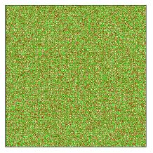
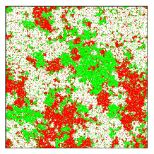
(a)                                   (b)

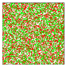
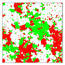
(c)                                   (d)

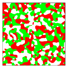
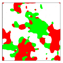
(e)                                   (f)

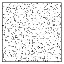
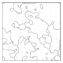
(g)                                   (h)

Figure 2: (Color online.) Snapshots of the $q=3$ ferromagnetic Potts model on a square lattice with linear size $L=1000$ after a quench, from initial states prepared at $T_{0}\rightarrow\infty$ (left column) and $T_{0}=T_{c}$ (right column), to the final temperature $T_{f}=T_{c}/2$. Times shown are, from top to bottom, $t=0,\ 2^{5}$ and $2^{10}$ MCs, respectively. In panels (g) and (h) the interfaces in the configurations at the latest time $t=2^{10}$ MCs [(e) and (f)] are shown, along with some small thermal fluctuations.

The initial conditions, either at critical ($2\leq q\leq 4$) or infinite temperature ($\forall\ q$), have very different characteristics and thus play an important role in the system’s evolution after the temperature quench, leading to very different dynamic structures. When a $2\leq q\leq 4$ model is in equilibrium at $T_{c}$ its configuration has long-range correlations. In $d=2$ the thermodynamic transition also corresponds to a percolation transition and one spanning cluster is already present in such initial conditions Vanderzande and Stella (1989); Saleur and Duplantier (1987); Janke and Schakel (2004); Picco et al. (2009). Naturally, such spanning clusters are not counted in our analysis since their perimeters would be severely under-estimated due to the finite system size. On the other hand, when the system presents a first order phase transition ($q>4$), the correlations are short-ranged at $T_{0}=T_{c}$ and the spanning cluster is not present initially nor at any time within the timespan (and system size) considered in our study. When the initial state is one of equilibrium at infinite temperature, $T_{0}\rightarrow\infty$, the correlations are absent and the model can be mapped onto random percolation. No spanning cluster is present initially for $q>2$ and none is generated during evolution (the case $q=2$ is subtly different, see Arenzon et al. (2007); Sicilia et al. (2007); Barros et al. (2009)). These distinctive features are made evident in the snapshots shown in Figs. 2 ($q=3$) and 3 ($q=8$), for the two initial conditions, infinite (left column) and critical temperature (right column).

For $q=3$, Fig. 2, the absence of correlations at $T_{0}\to\infty$ is clear from panel (a) while the long-range correlations and a spanning cluster present at $T_{c}$ can be easily visualized in panel (b). In panels (c) and (e) the snapshots show the thermal evolution after a quench from $T_{0}\to\infty$ to $T_{f}=T_{c}/2$ at times $t=2^{5}$ and $2^{10}$ MCs. In (d) and (f) the snapshots show the configurations at the same times after a quench from $T_{0}=T_{c}$. The perimeters of the domains at $t=2^{10}$ MCs are shown in (g) and (h). The right column panels demonstrate that the seeds for the large dynamic domains were already present in the initial condition and, although these objects do not translate during the evolution, they get rid of small, internal domains. Indeed, in the explored timespan, basically the modifications are that small domains are erased and the walls get smoother. A similar conclusion cannot be drawn from the left column snapshots as it is difficult to identify a seed for the structures seen at the latest time from the very disordered initial condition. A common feature of both $T_{0}=T_{c}$ and $T_{0}\to\infty$ evolved configurations is that domains with small areas have an approximately round shape. Instead, for large areas the pattern is rougher and one finds that these are sometimes stretched. A crossover in the morphology of the domains is determined by the characteristic length $R(t)$ and it will be discussed in Sec. III.

$T_{0}\to\infty$                            $T_{0}=T_{c}$

(a)                                   (b)

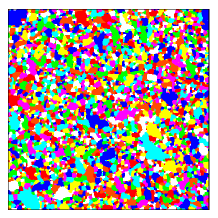
(c)                                   (d)

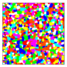
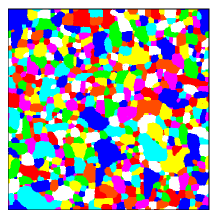
(e)                                   (f)

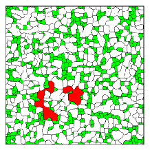
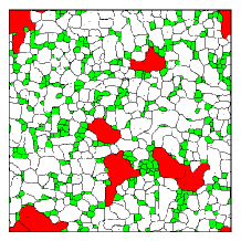
(g)                                   (h)

Figure 3: (Color online.) Sequence of snapshots for the $q=8$ Potts model. The left column displays results obtained by using an equilibrium initial configuration at $T_{0}\to\infty$ (a) and its time evolved after the quench [(c) and (e)]. The right column shows configurations found by using an equilibrium initial state at $T_{0}=T_{c}$ (b) and after the quench [(d) and (f)]. From top to bottom the measuring times are $t=0,\ 2^{7}$ and $2^{10}$ MCs, respectively, and $T_{f}=T_{c}/2$. In panels (g) and (h) we show the domains with areas $A<R^{2}$ (green, or light grey), $R^{2}(t)<A<10R^{2}(t)$ (white) and $A>10\ R^{2}(t)$ (red, or dark grey) for the configurations at $t=1024$ MCs.

Figure 3 shows a sequence of snapshots of the $q=8$ Potts model with both $T_{0}\to\infty$ (left column) and $T_{0}=T_{c}$ (right column) initial conditions. The quench is done to $T_{f}=T_{c}/2$, and the configurations at different times, $t=128$ MCs (second row) and $t=1024$ MCs (third row) are shown. Since none of the initial configurations is critical, thus having either a vanishing ($T_{0}\to\infty$) or a finite ($T_{0}=T_{c}$) correlation length, one might expect them to be statistically equivalent. However, the dynamically evolved configurations are different in at least two senses. First, the domains evolved from $T_{c}$ are larger, as can be clearly seen at naked eye. More importantly, the shape of the large domains are very different. Panels (g) and (h) take the configurations in panels (e) and (f) and color in the same way domains with areas $A<cR^{2}$ (green), $cR^{2}<A<10R^{2}$ (white) and $A>10R^{2}$ (red). In this way we highlight the density of domains with small, intermediate and large size as compared to the typical one, $R^{2}$, at the measuring time. On the one hand, when the initial state is uncorrelated (left column panels) few domains with area $A>10R^{2}$ survive at the latest time (two) and those have a stretched form. On the other hand, when the initial state is critical (panels in the right column) more domains remain at the chosen time (five), they have larger area and are usually less stretched. The difference will be made quantitative in Sec. III.1. It is clear from these figures that it is very hard to collect good statistics for large areas.

III Areas and Perimeters

In this section we analyze the relation between hull-enclosed areas and hull perimeters. For any sensible definition of volume and interface, the volume $V$ of a compact domain with a compact interface $S$ should satisfy

$$V\sim p^{d}\;,\qquad\qquad S\sim p^{d-1}\;,$$ (5)

with $p$ a linear dimension and $d$ the dimension of space, leading to

$$S\sim V^{1-1/d}\;.$$ (6)

However, if a domain has a fractal surface or holes (other domains) in its interior, Eqs. (5) are not necessarily valid Stauffer and Aharony (1994). In practice, the presence of holes inside domains depends on the dimension of space and the number of ground states of the system. While for $d=2$ and $q=2$ many domains have other internal domains Sicilia et al. (2007), for $d=2$ and $q\geq 3$ internal domains are much rarer (this can be checked from the snapshots in Fig. 3 for $q=8$). Therefore, domain areas and hull-enclosed areas differ by very little for $q\geq 3$ Loureiro et al. (2010). In the rest of this paper we focus on hull-enclosed areas and in this Section on their relation to the hull perimeters themselves.

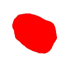
(a)                 (b)                 (c)

Figure 4: (Color online.) Examples of typical domain structures obtained in the simulations. In (a) a regular domain with area $A\sim p^{\alpha_{h}}$ and $\alpha_{h}=2$. The domain in (b) has a rougher morphology and a smaller exponent ${\alpha_{h}}$ certifies this feature, $1<{\alpha_{h}}<2$. In (c) a domain with very rough and stretched morphology, $A\sim p$; the exponent ${\alpha_{h}}$ reaches it minimum value, ${\alpha_{h}}=1$, in this case.

There are many possible definitions of a hull for a system defined on a lattice. We choose to use the one in which the hull perimeter is the number of sites that are on the external perimeter of a domain, see Fig. 1, matching the nomenclature in Stauffer and Aharony (1994).

III.1 Scaled scatter plots

We analyze scatter plots of areas vs. perimeters and their scaling properties. The results found in Sicilia et al. (2007) for the Ising case are extended in a natural way to the $q=3,\ 4$ cases as discussed below. Further subtleties are found in models with $q>4$ for which none of the initial states ($T_{0}=T_{c}$ and $T_{0}\to\infty$) are critical.

As in the Ising case, and independently of the initial condition having long or short range correlations, we can distinguish two types of domains depending on their relation to the characteristic length $R(t)$. Hull-enclosed structures with area $A<R^{2}(t)$ have a regular form and the area-perimeter relation is $A\sim p^{2}$ as in Eq. (5). Instead, domains with area $A>R^{2}(t)$ exhibit a rough surface and the area-perimeter relation keeps the power law form, $A\sim p^{{\alpha_{h}}}$, although with an exponent ${\alpha_{h}}<2$ that depends on the initial condition and $q$. Figure 4 shows examples of domains – taken from our simulations – with different exponents, ${\alpha_{h}}=2$ (a), $1<\alpha_{h}<2$ (b) and $\alpha_{h}\simeq 1$ (c). Once hull-enclosed areas and perimeters are measured with respect to the crossover value, itself written in terms of the characteristic length $R(t)$, we can write the scaling relation

$$\frac{A}{R^{2}}\sim\left(\frac{p}{R}\right)^{{\alpha_{h}}}\;,$$ (7)

where

$${\alpha_{h}}\left\{\begin{array}[]{lll}=2&\;\;\;\;\mbox{for}&A<R^{2}(t)\;,\\ <2&\;\;\;\;\mbox{for}&A>R^{2}(t)\;.\end{array}\right.$$ (8)

Figure 5 shows the rescaled relation (7) for $q=3$ after a quench from $T_{0}\rightarrow\infty$ to $T_{f}=T_{c}/2$ and several measuring times ($t=0,2,\ldots,2^{14}$ MCs). We used the characteristic length $R(t)\simeq(\lambda_{q}\ t)^{1/2}$ obtained from the analysis of the equal time correlation $C(r,t)$, as in Loureiro et al. (2010). The data collapse confirms that $A$ scales as $R^{2}$ and $p$ as $R$. We shall see below that this applies to all $q$ and to quenches from different initial conditions. While for small areas, $A<R^{2}(t)$, the exponent can be obtained from a fit performed on a conveniently long interval, for $A>R^{2}(t)$ the fitting interval is rather short. Nevertheless, the exponent obtained, ${\alpha_{h}}\simeq 1.06$, is so far from the regular value $2$, that we can definitely conclude that a change in morphology operates upon the domains at the crossover determined by $R(t)$. The domains with small areas are regular and $A\simeq p^{2}$. The ones with large areas are rough and stretched, the hull perimeters being very close to the hull-enclosed area itself, $A\simeq p$. The inset shows the raw data for the area $A$ versus the hull perimeter $p$ for $t=0$ to $t=2^{14}$ MCs (bottom to top). This figure confirms that during evolution the domains grow and become more regular. The red solid line is a guide-to-the-eye and represents $A\sim p^{2}$.

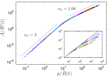
Figure 5: (Color online.) Scaling relation between hull-enclosed areas and hull perimeters at several measuring times for $q=3$ after a quench from $T_{0}\rightarrow\infty$ to $T_{f}=T_{c}/2$. The inset shows the raw data at several times from $t=0$ to $2^{14}$ MCs (bottom to top). The extent up to which the law $A\sim p^{2}$ (red solid line) applies increases with time, demonstrating that the domains become more regular in the course of evolution.

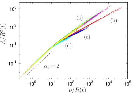
Figure 6: (Color online.) Scaling relation between hull-enclosed areas and hull perimeters at $t=2,\ldots,2^{10}$ MCs for different models (various $q$ values) and initial conditions. The curves labeled (a) correspond to $q=2,3,8$ and $T_{0}=T_{c}$, those labeled (b) are for $q=2$ and $T_{0}\rightarrow\infty$, the ones labeled (c) have been obtained using $q=3$ and $T_{0}\rightarrow\infty$ and, finally, the ones carrying the label (d) are for $q=8$ and $T_{0}\rightarrow\infty$. All quenches are to $T_{f}=T_{c}/2$. When the initial state is at the critical point, case (a), the relation $A\simeq p^{{\alpha_{h}}}$ presents a similar exponent for all $q$, ${\alpha_{h}}\simeq 1.44$. Instead, after a quench from the $T_{0}\rightarrow\infty$ uncorrelated state the exponent ${\alpha_{h}}$ decreases from its $q=2$ value ${\alpha_{h}}\simeq 1.15$ to ${\alpha_{h}}\simeq 1.06$. Notice that for the case $q=8$ and $T_{0}=T_{c}$, case (a), the observed exponent is 1.44 because the measure was taken at a relatively small time, in which the finite correlations present at the initial state are still large compared with the characteristic lenght. At later times, this exponent will decrease, eventually approaching 1.06, as the characteristic lenght grows beyond those initial correlations.

Next, in Fig. 6 we compare the relation between hull-enclosed areas and hull perimeters for systems with different values of $q$ quenched from different initial conditions. In all cases we find a power law relation, $A\simeq p^{\alpha_{h}}$, with varying values of ${\alpha_{h}}$. The group of curves labeled (a) corresponds to $q=2,\ 3$ and 8 quenched from $T_{0}=T_{c}$ to $T_{f}=T_{c}/2$ and the fit yields ${\alpha_{h}}\sim 1.44$. Interestingly, even the case $q=8$ with short-range correlation presents an exponent $\alpha_{h}>1$. On the other hand, when the initial state is one of infinite temperature, the exponent ${\alpha_{h}}$ is smaller and decreases with increasing number of states. In the first case (b) for $q=2$ we find ${\alpha_{h}}\sim 1.12$. For larger values of $q$ it is harder to be conclusive about the actual value of the exponent since the number of domains with area larger than $R^{2}$ decreases with increasing $q$ and the fitting interval gets smaller. Within our numerical accuracy, for $q=3$ (c) ${\alpha_{h}}\sim 1.06$ and for $q=8$ (d) ${\alpha_{h}}\lesssim 1.06$ but this value is not precise enough to be conclusive.

Summarizing, in all cases the characteristic length $R$ grows as $t^{1/2}$, the structures become more regular, and the power law $A\sim p^{2}$ for $A<R^{2}$ is more evident. Concomitantly, less domains have an area larger than $R^{2}$. For $T_{0}\to\infty$ the value of the exponent $\alpha_{h}$ characterizing the shape of the large hull-enclosed areas decreases with increasing $q$, consistent with $\alpha_{h}\to 1$ for $q\to\infty$. For $T_{0}=T_{c}$ the exponent $\alpha_{h}$ takes a higher value though still smaller than $2$ for large areas and, within our numerical precision, no dependence on $q$ for $q=2,\ 3$ and 8 was observed.

IV The von Neumann-Mullins law

The von Neumann-Mullins law, Eq. (1), predicts that each hull-enclosed area has a different rate of change depending only on its number of sides (and not on its area). This equation is not fully general; it has been derived under certain assumptions that include, as in the Allen-Cahn case Allen and Cahn (1979), the fact that the domain wall should be close to flat away from the triple points for $q>2$, a feature that can be achieved at long times and for long interfaces only. The law ruling the dynamics of small areas with highly curved interfaces or large areas with very rough walls is not known in general (in the Ising case, however, some exact results for small areas are known Kandel and Domany (1990); Chayes et al. (1995)). In this Section we numerically analyze the validity of the von Neumann-Mullins law by putting Eq. (1) and its average over small ($A_{0}<A<cR^{2}$) or large ($A>cR^{2}$) areas to the test ($A_{0}$ is a small area cut-off and $c$ a tunable parameter). We estimate the individual area time-derivate as $A_{i}(t+1)-A_{i}(t)$.

In Fig. 7 we examine Eq. (1) by plotting $dA/dt$ vs $A$ for $n=4$ and $n=8$ both at $t=1024$ MCs in a $q=8$ Potts model quenched from $T_{0}\to\infty$ to $T_{c}/2$ (similar ellipsoidal clouds are obtained for $T_{0}=T_{c}$ and for $q=3$). The vertical dashed line shows $R^{2}(t)\propto t$. The large vertical spreading of the data points let us conclude that the von Neumann-Mullins law does not hold strictly in our case, contrary to what was found in a phase field simulation of ideal grain growth Kim et al. (2006) and in a Potts models with very large $q$ and microscopic updates modified to ensure a local $q=6$ constraint and thus accelerate the evolution Kim (2010).

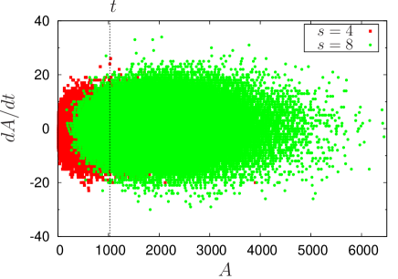
Figure 7: (Color online.) Rate of change of the individual hull-enclosed area at time $t=1024$ MCs after a quench from $T_{0}\to\infty$ to $T_{c}/2$ ($q=8$). The data are grouped by the number of sides $n=4$ (red, or dark grey) and $n=8$ (green, or light grey). The vertical dashed line indicates $R^{2}(t)\propto t$.

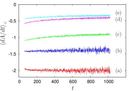
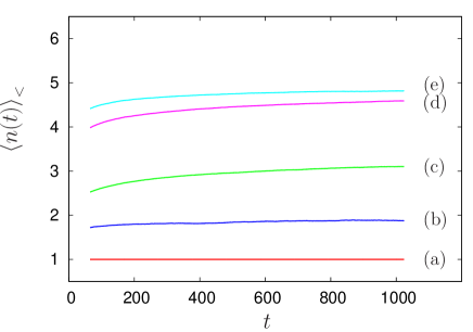
Figure 8: (Color online.) Top panel: The area rate of change averaged over small areas, $A_{0}=8<A<cR^{2}$, for (a) $q=2$ and $T_{0}\to\infty$ (red), (b) $q=3$ and $T_{0}=T_{c}$ (blue), (c) $q=3$ and $T_{0}\to\infty$ (green), (d) $q=8$ and $T_{0}=T_{c}$ (pink), and (e) $q=8$ and $T_{0}\to\infty$ (cyan). In all cases the averaged rate of change seems to asymptotically reach a negative constant. Bottom panel: The time-dependent average number of sides, $\langle n(t)\rangle_{<}$ for the same parameters is shown with the same color and label code. See the text for the discussion.

Figure 8 (top panel) shows the area rate of change averaged over small areas:

$$\left\langle\frac{dA}{dt}\right\rangle_{<}=\frac{1}{N_{<}(t)}\sum_{A_{0}<A_{i}<cR^{2}}\frac{dA_{i}}{dt}$$ (9)

where $N_{<}(t)$ is the number of areas obeying $A_{0}<A_{i}<cR^{2}$. When one area leaves the defining interval $[A_{0},cR^{2}]$, it is no longer taken into account in the sums; on the other hand, new areas can enter this interval. These are the reasons for the time-dependence in $N_{<}$. Each curve in the figure corresponds to different values of $q$ and temperature of the initial conditions: (a) $q=2$ at $T_{0}\to\infty$, (b) $q=3$ at $T_{0}=T_{c}$, (c) $q=3$ at $T_{0}\to\infty$, (d) $q=8$ at $T_{0}=T_{c}$ and (e) $q=8$ at $T_{0}\to\infty$. In cases (a) and (b) the averaged area rate of change has reached a constant (within the fluctuations). In the other cases, although the average continues to evolve within the explored time window, the variation is much smaller than the total mean area. In all cases $\langle dA/dt\rangle_{<}$ is negative and, according to the von Neumann-Mullins’s law, this implies an average number of sides smaller than 6. The fluctuations observed mainly in the case $q=3$ are the result of coalescence and dissociation processes that become increasingly rare as the number of ground states of the system increases.

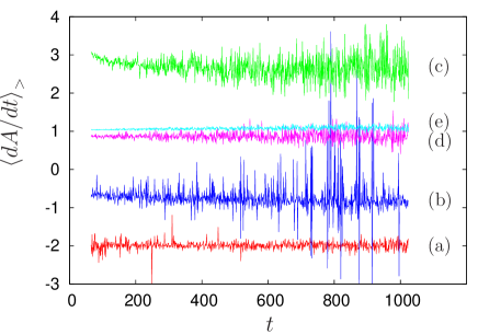
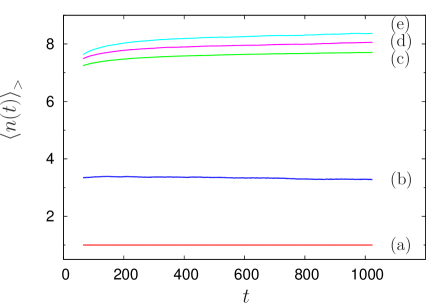
Figure 9: (Color online.) The same as in Fig. 8 but averaging over large areas, $A>cR^{2}$, for the same choice of parameters and color code used in that figure. Notice the order of the labels in the top panel.

The results in the top panel of Fig. 8 are to be compared to those in the bottom panel, where the small-area average of the time-dependent number of sides, $\langle n(t)\rangle_{<}$, is displayed. The results are qualitatively and quantitatively consistent with the averaged von Neumann-Mullins law

$$\left\langle\frac{dA}{dt}\right\rangle_{<}=\frac{\lambda_{q}}{5}\left(\langle n(t)\rangle_{<}-6\right)\;.$$ (10)

The values for $\lambda_{q}$ found by comparing the two sets of curves are consistent with $\lambda_{q}$ decreasing for increasing $q$ and independent of the initial temperature $T_{0}$, as is also found from the analysis of the space-time correlation function Loureiro et al. (2010).

The same analysis performed on the large areas is much more delicate. To start with, it is difficult to collect good statistics since only a few sufficiently large areas remain in the samples at long times, especially for large values of $q$. Figure 9 present data for the same set of parameters as in Fig. 8. Clearly, the fluctuations in the averaged area rate of change are much larger than when the average was performed over small areas. Still, one can argue that the rate of change asymptotically approaches a constant in all cases. However, and contrary to the small area case, the constant is negative only in the cases in which the initial state is critical ($q=3$ and 4, not shown, at $T_{0}=T_{c}$) and for the special case $q=2$ with $T_{0}\to\infty$. In all other cases [$q=3$, $T_{0}\to\infty$ (c), $q=8$, $T_{0}=T_{c}$ (d) and $q=8$, $T_{0}\to\infty$ (e)] the constant is positive. In cases (a) and (b) one finds agreement between the negative averaged area rate of change and the fact that the averaged number of sides of these areas is smaller than 6. Moreover, the $\lambda_{q}$ values found, within our numerical accuracy, are consistent with the ones stemming from the analysis of the data averaged over small areas.

The remaining three cases have to be discussed separately. While the signs are consistent, i.e. positive averaged area rate of change and average number of sides larger than 6, the trend of these curves is not systematic and shows that such large structures do not follow the linear behavior predicted by the von Neumann-Mullins law. This might be due to different reasons. For instance, in the case $q=3$ with $T_{0}\to\infty$ (c) we ascribe this feature to the fact that the long-time domain structure is special in this case, with many large domains with a rather rough surface, as shown in panel (e) of Fig. 2 and confirmed by the fact that $\alpha_{h}$ is very close to one, see Fig. 5, in this regime.

Figure 10 display the total number of hulls with $n$ sides, $N_{h}(n,t)$, in a log-log scale, showing the behavior at four different times, for $q=3$ after a quench from $T_{0}\rightarrow\infty$ (solid symbols) and $T_{0}=T_{c}$ (empty symbols) to $T_{f}=T_{c}/2$. The dotted horizontal and vertical lines indicate $N_{h}=1$ and $n=6$, respectively. For initial conditions with finite correlation length (upper group of curves) many interfaces have more than 6 sides and the average value $\langle n\rangle$ is less representative of the fluctuating behavior. The distribution tail seems exponential. Instead, for critical initial conditions (lower group of curves), the number of hulls with 6 or more sides becomes negligible during evolution and the distribution decays as a power law. Interestingly, for $T_{0}\to\infty$ the curves are monotonically decreasing for $n\geq 4$ while for $T_{0}=T_{c}$ they are monotonically decreasing for $n\geq 2$ (note that for the case $q=3$ shown here, $n$ only takes even values). The former feature is experimentally established although it is not captured by simplified random neighbor models Flyvbjerg (1993); Durand (2010).

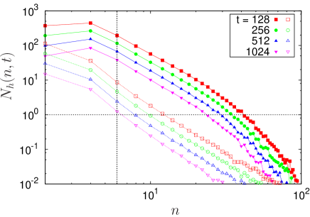
Figure 10: (Color online.) Total number of hulls with $n$ sides for $q=3$, $T_{0}\to\infty$ (solid symbols, upper group of curves) and $T_{0}=T_{c}$ (empty symbols, lower group of curves). The dotted lines indicate $N_{h}=1$ (horizontal) and $n=6$ (vertical). The different symbols correspond to different measuring times as given in the key. The distribution has weight well above $N_{h}=1$ for $n>6$ when the initial conditions have finite correlation length.

The summary of our analysis of the von Neumann-Mullins law is given in Fig. 11 where we averaged the area rate of change over all areas with given value of $n$ and displayed the results as a function of $n$ for the $q=3$ and $q=8$ models quenched from $T_{0}=T_{c}$ and $T_{0}\to\infty$. The data are measured at $t=64$ MCs. Although the $n-6$ dependence is observed for both values of $q$ and the different initial conditions, the behavior is linear in the averaged data only up to $n\simeq 10$ (lower solid straight line). Deviations appear for larger values of $n$ in all cases.

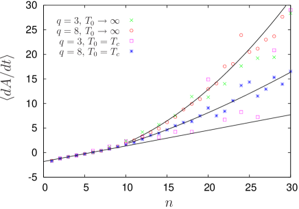
Figure 11: (Color online.) The full averaged area rate of change as a function of the number of sides at $t=64$ MCs for the parameters given in the key. The solid lines correspond to the function $f(x)\simeq x^{\gamma}$ with $\gamma=1,\ 1.5,\ 2$, from bottom to top, and serve as guides to the eyes.

V Hull perimeter distributions

In a previous work, Ref. Loureiro et al. (2010), the hull-enclosed area distribution, $n_{h}(A,t)$, was studied for the $q$-state Potts model after temperature quenching the system from above the critical temperature into the ordered phase. We now describe the time evolution of the hull perimeter distribution, $n_{h}(p,t)$, following this quench and relate it to $n_{h}(A,t)$. The form of the distribution depends on the initial condition and on the value of $q$. In particular, there is a dependence on the morphological characteristics of each domain, that are different for structures with large or small sizes, when compared to the characteristic lenght $R(t)$.

V.1 Critical initial condition

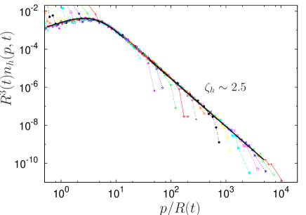
Figure 12: (Color online.) Rescaled hull perimeter distribution for $q=3$ at several times ($t=2,2^{2},\ldots,2^{14}$ MCs), after a quench from $T_{0}=T_{c}$ to $T_{f}=T_{c}/2$. The solid black line represents the theoretical prediction, Eq. (12), valid for small areas, $A/R^{2}<10$ with $\alpha_{h}=2$ and for large areas, $A/R^{2}>10$, with $\alpha_{h}\simeq 1.44$.

For $2\leq q\leq 4$ the transition is continuous and the initial state at $T_{0}=T_{c}$ is critical; hence all initial distributions, i.e. of areas and perimeters, should have a power law tail. The functional form of the equilibrium number density of hull-enclosed areas at $t=0$ is $n_{h}(A,0)=(q-1)c^{(q)}_{h}/A^{2}$ Loureiro et al. (2010). Since one and only one hull is associated to each hull-enclosed area, the number density of hull perimeters should be linked to the one of hull-enclosed areas according to $n_{h}(p,0)dp=n_{h}(A,0)dA$. Using $A\simeq p^{\alpha_{h}}$, a relation that is valid one-to-one, one finds

$$n_{h}(p,0)\sim\frac{\gamma_{q}}{p^{\zeta_{h}}}\;.$$ (11)

where $\gamma_{q}=\alpha_{h}(q-1)c^{(q)}_{h}$ and $\zeta_{h}=\alpha_{h}+1$. The exponent $\zeta_{h}$ is the equivalent to the Fisher exponent $\tau$ for the area distribution now describing the perimeter distribution. In two dimensions $\zeta_{h}$ is linked to the fractal dimension of the perimeter $D_{h}$ as Stauffer and Aharony (1994) $\zeta_{h}=1+2/D_{h}$. In the special case $q=2$ at $T_{c}$ one has $D_{h}=11/8$ Vanderzande and Stella (1989).

Using the fact that areas and perimeters are related one to one also dynamically, $n_{h}(p,t)dp=n_{h}(A,t)dA$, and the power-law relation between areas and perimeters, Eq. (7), the time-dependent number density of hull perimeters can be easily written as

$$n_{h}(p,t)\sim\dfrac{\gamma_{q}}{R^{3}}\;\dfrac{\left(\dfrac{p}{R}\right)^{\alpha_{h}-1}}{\left[1+\left(\dfrac{p}{R}\right)^{\alpha_{h}}\right]^{2}}\;.$$ (12)

The value of $\alpha_{h}$ depends on which of the two regimes, $p<R$ and $p>R$, one focuses on, with $\alpha_{h}=2$ in the former and $\alpha_{h}<2$ in the latter. A similar argument was used in Sicilia et al. (2007) and Sicilia et al. (2009) to obtain the perimeter number density in the $2d$ Ising model with non-conserved and conserved order parameter dynamics, respectively.

Figure 12 shows the hull perimeter number density, scaled by the characteristic length $R(t)$, for the critical model with $q=3$ after a quench to $T_{f}=T_{c}/2$. The long-range correlations present in the critical initial state are preserved during evolution and lead to the power law tail in the distribution. The exponent of this tail is $\zeta_{h}\sim 2.5$ in agreement with the theoretical estimate $\zeta_{h}=\alpha_{h}+1\simeq 1.44+1$, see Fig. 6. For small areas, $p\ll R$, one finds $R^{3}n_{h}(p,t)\simeq\gamma_{q}p/R$ also in good agreement with the analytic prediction. Thus, equation (12) describes well these two limits.

V.2 Non-critical initial condition

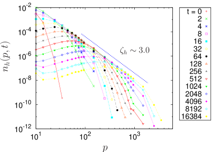
Figure 13: (Color online.) Hull perimeter distribution for $q=8$ at several times given in the key after a quench from equilibrium at $T_{0}\rightarrow\infty$ to $T_{f}=T_{c}/2$. The declivity of the envelope, $\zeta_{h}\sim 3.0$, is a direct consequence of dynamical scaling.

Being far from critical percolation, the initial state at $T_{0}\to\infty$ for a system with $q>2$ does not become critical during its evolution and the area (and consequently the perimeter) distribution does not develop a power law tail. In Fig. 13 we use log-log scale to show the $q=8$ hull perimeter distribution after a quench from $T_{0}\rightarrow\infty$ to $T_{f}=T_{c}/2$ at several times. Similarly to what happens with the hull enclosed area distribution for $q>2$ Loureiro et al. (2010), there is a $p^{-3}$ envelope that is a consequence of dynamical scaling.

For very large $q$, after the quench, domains start to increase from localized density fluctuations that are randomly scattered throughout the system, in a similar way to the Avrami-Johnson-Mehl method Ferenc and Néda (2007) used to produce Voronoi diagrams. Thus, neglecting coalescence effects that are only important for small $q$, it can be conjectured that the set of domain centers (defined, for example, as the center of mass of a domain) may be approximately described as a set of random points from which Voronoi domains are drawed. Indeed, as we show in Fig. 14 for $q=8$ (see also Ref. Loureiro et al. (2010)), the distribution of areas after a temperature quench from $T_{0}\to\infty$ to $T_{c}/2$, is well described by the generalized Gamma (or Voronoi) distribution Ferenc and Néda (2007), widely used in grain growth literature Norbakke et al. (2002); Wang and Liu (2003); Xiaoyan et al. (2000); Kim (2010):

$$n_{h}(A,t)\sim\left(\frac{A}{R^{2}}\right)^{a-1}\exp\left[-b\left(\frac{A}{R^{2}}\right)^{c}\right],$$ (13)

with $a\simeq 1.21$, $b\simeq 1.22$, $c\simeq 0.6$. Simpler versions of the above function have also been proposed, with two ($c=1$) or a single ($c=1$ and $a=b$) parameter. Indeed, the values that we get for $a$ and $b$ are almost the same, but $c\neq 1$.

Once the distribution of areas is known, in principle one could relate it, as in the preceeding section, to the perimeter distribution using Eq. (7), obtaining, once again, a Gamma distribution:

$$n_{h}(p,t)\sim R\left(\frac{p}{R}\right)^{\alpha_{h}a-1}\exp\left[-b\left(\frac{p}{R}\right)^{\alpha_{h}c}\right].$$ (14)

Differently from the area distribution, the dependence on $\alpha_{h}$ characterizes two distinct regimes, $\alpha_{h}=2$ for $p<R$ and $\alpha_{h}<2$ for $p>R$. As one can see from Fig. 13, the data are well described by the above distribution. However, the fit parameters are not only different from those obtained from the area distribution but differ as well between the regions with small and large $p$. One possible reason is that although Eq. (13) is a good approximation, the dynamics of a growing domain is not equivalent to the Avrami-Johnson-Mehl method. If the Voronoi cells of the domain centers are drawn, there will be a large superposition with the actual domains, but those regions close to the interfaces could be wrongly assigned because, differently from Voronoi diagrams in which the borders are as straight as they can be on a lattice, a coarsened domain has rougher interfaces. Thus, the deviations are on the scale of the perimeter lenght and, although they may not be noticeable for area distributions, they become visible in the perimeter distributions.

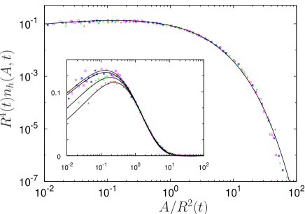
Figure 14: (Color online.) Hull-enclosed area distribution for $q=8$ at several times after a quench from equilibrium at $T_{0}\rightarrow\infty$ to $T_{f}=T_{c}/2$, rescaled by $R^{2}(t)$. The solid line is a fit with Eq. (13) and $a\simeq 1.21$, $b\simeq 1.22$, $c\simeq 0.6$. Inset: the same data in a linear scale, showing that for small areas, the collapse improves at large times.

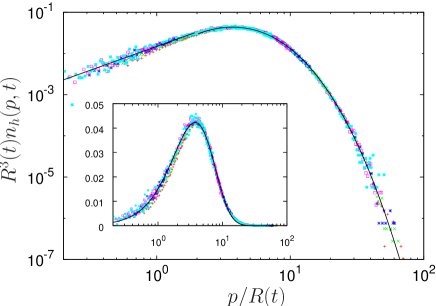
Figure 15: (Color online.) Hull perimeter distribution for $q=8$ at several times after a quench from equilibrium at $T_{0}\rightarrow\infty$ to $T_{f}=T_{c}/2$, rescaled by $R(t)$. The solid line is Eq. (14) with $\alpha_{h}=2$ for $p<R$ and $\alpha_{h}\simeq 1.06$ for $p>R$. The fit parameters, however, besides being different from those of Fig. 14, differ also for $p<R$ and $p>R$. Inset: the same data in a linear scale.

VI Conclusions

We studied several geometric properties of the nearest-neighbour $q$-state Potts model quenched below its phase transition. In particular we analyzed the von Neumann-Mullins law, the hull perimeter length distribution and the relation between hull perimeters and their enclosed areas. Diversely from the so called cellular Potts model, in which several layers of interacting neighbours are considered in order to decrease the lattice anisotropy, here it is an important ingredient. Moreover, coalescence is also relevant when $q$ is not too large, as the values considered here. These two factors, necessary for the single domain von Neumann-Mullins law, are here violated and deviate the model from the ideal grain growth conditions.

After having confirmed that all dynamic observables satisfy dynamic scaling with respect to the growing length $R(t)\simeq(\lambda_{q}t)^{1/2}$, we studied the fractal properties of the hulls by plotting $A/R^{2}(t)$ against $(p/R(t))^{\alpha_{h}}$, Eq. 7. We found that for $p/R(t)\ll 1$ interfaces are smooth with $\alpha_{h}=2$ while for $p/R(t)\gg 1$ they are fractal with $\alpha_{h}$ being smaller for $T_{0}\to\infty$ than for $T_{0}=T_{c}$ and decreasing with $q$. Thus, the behavior of objects with linear sizes that are smaller that the typical growing length have a rather different dynamics, morphology and statistical properties than those whose linear sizes are larger than the dynamical length.

The linear proportionality between $dA/dt$ and $n$ (independently of $A$), the von Neumann-Mullins law, does not hold for each individual area for the nearest neighbour Potts model in the temperature interval considered here after the quench. This may be due to thermal fluctuations occuring along the perimeter that may mask the curvature driven contribution. We then examined the law on the mean, by averaging over areas that are smaller or larger than the typical one, $R^{2}(t)$. In the small area regime the linear von Neumann-Mullins law is verified on the mean while for larger areas it is not, with deviations from linearity depending on the value of $q$ and initial conditions. The same separation of regimes is found when averaging over all areas that have the same number of sides. The behavior at large values of $n$ seems to be captured by a modified power law involving $\alpha_{h}$ but our data are not extensive enough to test this conjecture.

Finally, we studied the hull perimeter distribution distinguishing critical ($T_{0}=T_{c}$ for $q\geq 4$) from non-critical (all other cases, especially large $q$ for $T_{0}\to\infty$). In the former case we found that the scaling function can be derived with an argument that combines the use of Eq. (7) with the form of the distribution of hull-enclosed areas found in Ref. Loureiro et al. (2010). For non-critical initial conditions we found, instead, that the Gamma function commonly used in studies of ideal grain growth describes well both the hull-enclosed area and perimeter distributions, although the expected relation between the exponents of both distributions is not obeyed. The reason is due to the fact that the perimeter distribution is much more sensitive to the differences between the actual domains and their Voronoi approximations, as discussed in section V.2.

There are, however, several statistical properties of interface sides and topological properties for cellular systems that were not yet fully studied for the nearest-neighbour Potts model, and will be the subject of a future publication.