Baryon Content of Massive Galaxy Clusters at $z=0-0.6$

Abstract

We study the relationship between two major baryonic components in galaxy clusters, namely the stars in galaxies, and the ionized gas in the intracluster medium (ICM), using 94 clusters that span the redshift range $0-0.6$. Accurately measured total and ICM masses from Chandra observations, and stellar masses derived from the Wide-field Infrared Survey Explorer and the Two-Micron All-Sky Survey allow us to trace the evolution of cluster baryon content in a self-consistent fashion. We find that, within $r_{500}$, the evolution of the ICM mass–total mass relation is consistent with the expectation of self-similar model, while there is no evidence for redshift evolution in the stellar mass–total mass relation. This suggests that the stellar mass and ICM mass in the inner parts of clusters evolve differently.

1. Introduction

The baryon content in groups and clusters of galaxies is one of the basic quantities that could be used to test models of structure formation. The total baryon mass fraction in massive clusters has been used to estimate cosmological parameters (e.g., White et al., 1993; Allen et al., 2004). The mass of stars in galaxies is a fossil record of the star formation and galaxy merger history (Conroy et al., 2007). The relative proportion in mass of hot (diffuse intracluster medium, ICM) and cold baryons (e.g., stars in galaxies) could be used to gauge the strengths of various feedback mechanisms and star formation efficiency (e.g., Bode et al., 2009).

Although many measurements of the baryon fraction in local clusters exist (e.g., Lin et al., 2003; Gonzalez et al., 2007; Andreon, 2010; Balogh et al., 2011), such studies using large cluster samples at higher redshifts are in short supply. The first attempt has been made with the X-ray selected groups at $z=0.1-1$ detected in the COSMOS field (Giodini et al., 2009, hereafter G09). However, the total and ICM masses are not well-measured for individual systems, so G09 could not constrain $M_{\rm ICM}/M_{\rm star}$ well, especially at the massive end (see also Leauthaud et al. 2011).

Here we present a measurement of the baryon mass fraction contained in galactic stars and ICM, as well as the relationship between $M_{\rm ICM}$ and $M_{\rm star}$, using 94 clusters at $z\leq 0.6$ – the largest sample with accurate total and ICM mass measurements to date for this purpose. For the $z>0.1$ systems, we use data from the Wide-field Infrared Survey Explorer (WISE; Wright et al. 2010) survey to determine $M_{\rm star}$, while for the local clusters, we rely on data from the Two-Micron All-Sky Survey (2MASS, Skrutskie et al. 2006). To ensure uniformity of our measurements and to facilitate comparison across the cosmic epochs, all quantities are measured within $r_{500}$, the radius within which the mean overdensity is 500 times the critical density of the Universe $\rho_{c}$ at the cluster redshift.

In this paper we have neglected neutral and molecular gas in the baryon budget, as their amount is believed to be small (e.g., Chung et al., 2009). Our analysis does not include the intracluster stars either (as they are well below the surface brightness limit of WISE), although they may contribute a non-negligible fraction to the total cluster stellar mass (e.g., Gonzalez et al., 2007). Throughout this paper we adopt a WMAP-5 (Komatsu et al., 2009) $\Lambda$CDM cosmological model where $\Omega_{M}=1-\Omega_{\Lambda}=0.26$, $H_{0}=71h_{71}\,{\rm km\,s}^{-1}{\rm Mpc}^{-1}$.

2. Analysis Overview

Our analysis relies on the X-ray measurements to provide the cluster center, size, and the mass of the ICM. The cluster samples used are described in §2.1. We discuss the way artifacts and stars are rejected from the WISE catalogs in §2.2. Throughout this study we only make use of WISE 3.4 $\mu$m data. For each cluster, we use the background-subtracted total flux to estimate the total cluster luminosity and stellar mass. The method is described fully in Lin et al. (2003, 2004). In §2.3 we outline our modified procedures for analyzing the WISE data.

2.1. Cluster Samples

We assemble our intermediate redshift ($z=0.1-0.6$) cluster sample from Maughan et al. (2008, hereafter M08) and Vikhlinin et al. (2009, hereafter V09), both of which are based on Chandra observations. Although the 115 clusters from M08 are a heterogeneous sample (selected to be targeted ACIS-I observations, at $z>0.1$, publicly available in Chandra archive as of 2006), the large sample, analyzed in a uniform fashion, is advantageous, and allows us to probe the baryon content in clusters of various dynamical states. The Chandra subsample of the ROSAT PSPC 400 deg² survey presented in V09, on the other hand, has a well-defined selection function, but is smaller in size (41 objects). We have taken from these studies the X-ray center, ICM and total mass. The total mass $M_{500}$ is derived from the $Y_{X}$–$M_{500}$ relation (Kravtsov et al., 2006), where $Y_{X}$ is the product of core-excised X-ray temperature $T_{X}$ and $M_{\rm ICM}$. Using clusters common in the two samples we have verified that the two analyses yield measurements consistent to $\lesssim 5\%$. Requiring that the clusters are fully covered in the WISE Preliminary Data Release (PDR) footprint (see below), and are not affected by nearby bright stars, our final sample consists of 45 clusters, with 29 and 16 clusters from M08 and V09, respectively.

As our local ($z<0.1$) benchmark, we combine the cluster sample presented in Lin et al. (2004, hereafter L04) with the low-$z$ systems from V09. The resulting 49 clusters have accurate total and ICM mass measurements from Chandra or ROSAT, as well as total stellar mass estimates based on the near-IR $K_{s}$-band luminosity from 2MASS.

2.2. WISE Data

WISE is a satellite mission to survey the whole sky in four infrared bands (3.4, 4.6, 12, and 22 $\mu m$; hereafter W$1-4$), with a limiting magnitude of 17 (Vega) in W1. The recent PDR has made public reduced images and source catalogs for 57% of the sky. For each cluster we query the NASA/IPAC Infrared Science Archive (IRSA) to download WISE PDR source catalog out to $5-10r_{200}$, where $r_{200}$ is a proxy of the cluster virial radius, within which the mean overdensity is $200\rho_{c}$, and is extrapolated from $r_{500}$ by assuming an Navarro et al. (1997, hereafter NFW) density profile with concentration $c=5$. The large area surrounding the clusters is used for estimating the local background galaxy count and flux. In practice the background is estimated with an annulus with the inner and outer radii set to be four and five times $r_{200}$, respectively, although the exact choices vary from cluster to cluster, primarily depending on the distribution of bright star masks. Our results are not sensitive to the exact choice of the annulus radii. We only use objects without any known artifacts in W1 and W2.

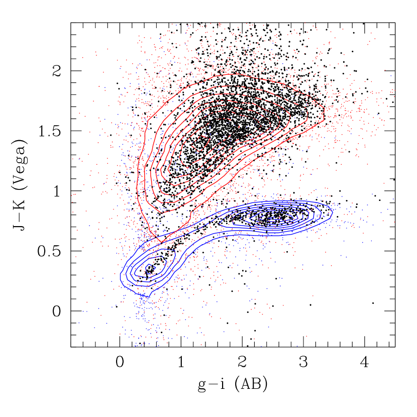
Figure 1.— The blue and red contours and points show the stellar and galaxy loci, combining data from SDSS and UKIDSS DXS. The black points are the WISE objects without a match in the 2MASS point source catalog. Only 7% of such WISE sources lie along the stellar locus, which suggests that stellar contamination in our WISE galaxy catalogs is $\leq 7\%$.

Because of its $6\arcsec$ FWHM point spread function (PSF), WISE does not provide useful morphological information to allow distinction between point and extended sources. Instead, we use 2MASS data to help select galaxies. Specifically, for each cluster we download the 2MASS point source catalog from IRSA, covering the same area as the WISE data. We then regard every WISE object with a 2MASS match within $2\arcsec$ as point-like and remove them from our catalog.

To evaluate the efficiency of this approach in star-galaxy separation, we use a 1.5 deg² region located in the XMM-LSS field that has deep optical and near-IR data from CFHTLS Wide (Gwyn, 2011) and UKIDSS DXS (Lawrence et al., 2007) surveys. In Fig. 1 we show the distribution of the stellar and galaxy loci on the $g-i$ vs $J-K$ diagram, obtained by cross matching the SDSS star and galaxy catalogs (Aihara et al., 2011) with DXS data. We overlay the 7163 WISE sources without a match in the 2MASS point source catalog, and find that only 7% of them lie on the stellar locus. This shows that using 2MASS we can remove the great majority of the stars. For the remaining stars in our catalogs, we remove their contribution via statistical background subtraction.

2.3. Estimating Total Luminosity and Stellar Mass

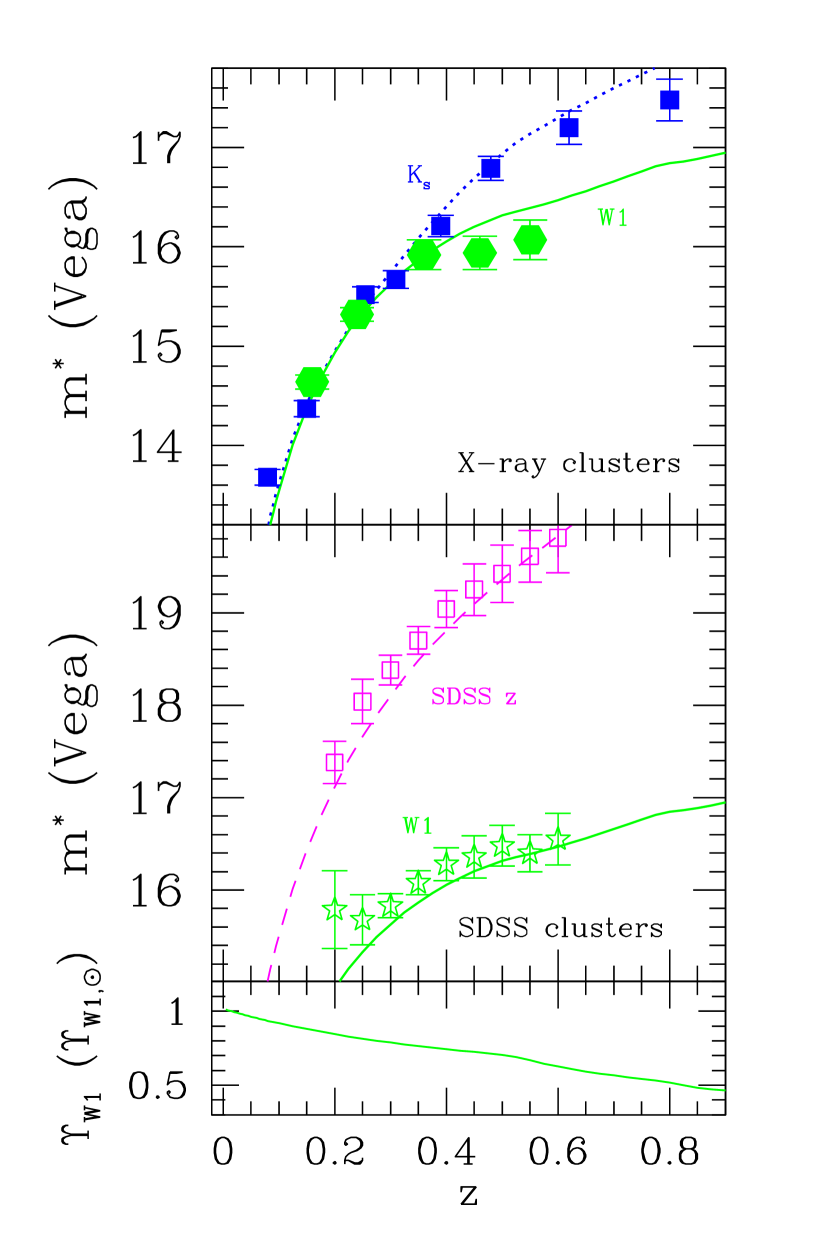
Figure 2.— Upper panel: Evolution of the apparent characteristic magnitude $m^{*}$ of the cluster galaxy LF in $K_{s}$-band (blue/solid squares; from Lin et al. 2006) and W1 (green/solid circles; our X-ray cluster sample). The dotted and solid curves show the predictions in $K_{s}$ and W1 of a single stellar population formed at $z=3$ with the Kroupa initial mass function and an exponentially decaying star formation history, normalized to fit the $K_{s}$-band data. Middle panel: $m^{*}$ of the cluster galaxy LF in $z$-band (magenta squares) and W1 (green stars) for the optical clusters from Geach et al. (2011). The two curves are the predictions of the same population synthesis model in $z$-band and W1. Lower panel: evolution of stellar mass-to-light ratio in W1.

To describe the evolution of the cluster galaxy populations, as well as for the $k$-correction, we use a simple stellar population evolution model based on an updated version of the Bruzual & Charlot (2003) population synthesis software package (hereafter the BC model). The model is a single stellar population of solar metallicity formed at $z=3$ with an exponentially decaying star formation history (with an $e$-folding timescale $\tau=0.1$ Gyr), with the Kroupa initial mass function (IMF), normalized to fit the apparent characteristic magnitude $m^{*}$ in the $K_{s}$-band for massive X-ray clusters at $z=0.1-0.8$, which are taken from Lin et al. (2006, hereafter L06). Using the BC model, we follow L06 to construct the composite W1 luminosity functions (LFs) in observer’s frame in five redshift bins. For each bin, we calculate the mean redshift of the clusters $z_{m}$, and adjust the $k$-correction and distance modulus of individual clusters to best represent how the clusters would appear if they were all at $z_{m}$. We then fit the composite LFs with the Schechter (1976) function, and show the best-fit $m^{*}$ in Fig. 2 (top panel).

For the lower three redshift bins, the W1 $m^{*}$ evolution agrees well with the BC model. For the two higher redshift bins, the observed $m^{*}$ is about 0.3 mag brighter than the model. To check if this is resulted from the blending of galaxies due to the large PSF of WISE, we also construct composite LFs in the SDSS $z$-band and W1 for a sample of $\sim 900$ optically-selected clusters and groups located in SDSS stripe 82, using the catalog of Geach et al. (2011, hereafter G11). The $m^{*}$ measured for these clusters is shown in the middle panel of Fig. 2, along with the BC model predictions. Although the measured $m^{*}$ of the SDSS clusters are slightly fainter than the predictions, the general agreement of $m^{*}$ in both W1 and $z$-band with the models indicates that blending is not the cause of the $m^{*}$ being brighter than the models for our X-ray cluster sample at $z>0.4$. The galaxies in our X-ray clusters are indeed more luminous on average than those in the SDSS optical clusters; for example, the mean difference of the magnitudes of the brightest cluster galaxies between the two samples is about 1 mag. This is not surprising given that our clusters are more massive than the G11 sample on average (see e.g., L04, Hansen et al. 2009). With the chosen BC model, our evolving $m^{*}(z)+2$ flux threshold (see below) corresponds to a constant galaxy stellar mass limit of $2\times 10^{10}M_{\odot}$. For this reason, and for sake of consistency, we will use the BC model for the $k$-correction and $m^{*}$ evolution, but will comment below on the impact of the “brightening” of galaxies in $z>0.4$ clusters on our results.

For each cluster, we sum the fluxes from objects brighter than the smaller of $m^{*}(z)+1.5$ and W1$=17.0$, and subtract fluxes from similar objects located within the background annulus (scaled by the relative area of the annulus and cluster region). Assuming all clusters have the same shape of LF (with a faint-end power-law slope $\alpha=-0.9$), which is consistent with our data (see also L06), we convert the background subtracted flux to $L_{{\rm tot}}$ using an NFW profile with $c=5$, defined as the total luminosity from all galaxies located within $r_{500}$ that are more luminous than $M^{*}(z)+2$. On average the conversion from observed to total luminosity requires only 15% of extrapolation. For reference, at $z=0$ we have $\Upsilon_{\rm 0,W1}=1.01M_{\odot}/L_{\odot,{\rm W1}}$.

For our $z<0.1$ clusters, we measure the total luminosity in the $K_{s}$-band using 2MASS data (following L04); Again $M_{{\rm star}}=L_{{\rm tot}}\Upsilon_{K_{s}}(z)$, using the $K_{s}$-band $\Upsilon_{K_{s}}(z)$ from the same BC model. Our stellar mass estimates are consistent with that listed in Lin et al. (2003), and are similar to that of Andreon (2010) and Gonzalez et al. (2007), when the intracluster light (ICL) contribution is excluded from the latter study. For a few clusters at $z<0.1$ we have also used WISE data to estimate $M_{\rm star}$, and found agreement with 2MASS-based values to within 10%.

3. Correlations between Stellar Mass, ICM Mass, and Total Mass

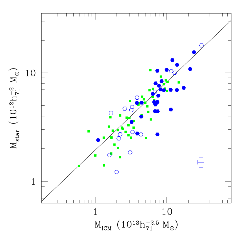
Figure 3.— Correlation between the total stellar mass and ICM mass, both measured within $r_{500}$, for the M08 clusters (filled circles), V09 clusters (open points), and $z<0.1$ clusters (green/squares). To avoid overcrowding the plot, errorbars for a typical cluster are shown in the lower right corner. We include a 10% uncertainty in stellar mass for the assumption that a single value of mass-to-light ratio can describe the bulk of galaxies in a cluster. The choice of the IMF is the largest systematic uncertainty, at the 30% level. The line is the best-fit to clusters at $z\sim 0$ (Eqn. 3).

In Fig. 3 we show the $M_{\rm star}$–$M_{\rm ICM}$ correlation, measured within $r_{500}$, for the M08 clusters (filled circles), V09 clusters (open points), and $z<0.1$ clusters (green squares). The M08 and V09 samples, although constructed using different selection criteria, appear to follow the same trend. Together the sample spans a factor of 30 in $M_{{\rm ICM}}$, allowing us to determine the slope of scaling relations well.

The correlations between the baryon components and the cluster mass are shown in Fig. 4. The lower sets of points are the stellar mass fraction ($f_{\rm star}=M_{\rm star}/M_{500}$), and the upper sets are the baryon fraction, $f_{\rm b}=(M_{\rm ICM}+M_{\rm star})/M_{500}$, which is dominated by the ICM.

To investigate any redshift evolution among these correlations, we fit the data with the following form by $\chi^{2}$ minimization, taking into account the uncertainties in both mass measurements:

$$M_{\rm star} \propto M_{\rm ICM}^{s_{1}}(1+z)^{\gamma_{1}}$$

$$M_{\rm star} \propto M_{500}^{s_{2}}(1+z)^{\gamma_{2}}$$

$$M_{\rm ICM} \propto M_{500}^{s_{3}}(1+z)^{\gamma_{3}}.$$ (1)

We find that $\gamma_{1}=-0.31\pm 0.22$, $\gamma_{2}=-0.06\pm 0.22$, and $\gamma_{3}=0.41\pm 0.14$; $s_{1}=0.62\pm 0.04$, $s_{2}=0.71\pm 0.04$, and $s_{3}=1.13\pm 0.03$. That is, there is no evolution for the $M_{\rm star}$–$M_{500}$ relation, weak suggestion of evolution in $M_{{\rm star}}$–$M_{{\rm ICM}}$, and strong evidence of evolution in $M_{\rm ICM}$–$M_{500}$, which is manifested as an offset between the loci of $f_{\rm b}$ for $z<0.1$ (solid squares) and $z>0.1$ (circles) clusters in Fig. 4. This is mainly due to the self-similar evolution (SSE) of the ICM, as noted first by V09 (see the discussion associated with Fig. 10 therein). Let us denote $M_{\rm ICM}\propto M_{500}^{1+\kappa}$, where $\kappa\equiv s_{3}-1=0.13$ based on our data. Introducing the nonlinear mass scale, $M_{\rm NL}$, satisfying $\sigma(M_{\rm NL})D(z)=\delta_{c}\approx 1.69$, where $\sigma(M)$ is the rms fluctuation of linear power spectrum and $D$ is the growth factor (Peebles, 1980), we can expect the ICM mass fraction to be the same for systems of the same $M_{500}/M_{\rm NL}$ at different redshifts under the SSE. It then follows that $M_{\rm ICM}\propto M_{500}^{s_{3}}/M_{\rm NL}^{\kappa}$. We note that $M_{\rm NL}(z)^{-\kappa}$ is consistent with $(1+z)^{\gamma_{3}}$ up to $z\sim 0.4$ or so. Indeed, with total mass scaled by $M_{\rm NL}$, the scatter reduces from 12% to 8%. We have confirmed the consistency between the observed $M_{\rm ICM}$–$M_{500}$ evolution and the SSE expectation by repeating the above analysis using $M_{500}$ based on the $T_{X}$–$M_{500}$ relation of V09.

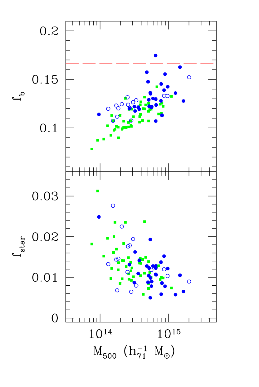
Figure 4.— The upper panel shows the baryon mass fraction, while the lower panel shows the stellar mass fraction. The solid (open) circles are M08 (V09) clusters, and the solid squares are $z<0.1$ clusters. The horizontal dashed line is the cosmic baryon fraction from WMAP (Komatsu et al., 2009). No attempt has been made to include the contribution from the ICL.

Using all of the clusters we find that

$$\frac{M_{{\rm star}}}{10^{12}h_{71}^{-2}M_{\odot}} = \left(1.9\pm 0.1\right)\left(\frac{\Upsilon_{\rm 0,W1}}{1.0\Upsilon_{\odot,{\rm W1}}}\right)$$

$$\mbox{}\times\left(\frac{M_{{\rm ICM}}}{10^{13}h_{71}^{-2.5}M_{\odot}}\right)^{0.62\pm 0.04}\left(1+z\right)^{-0.31\pm 0.22}$$

with a scatter of 31%; Without strong evidence of evolution, for simplicity we take $\gamma_{2}=0$ in Eqn. 3 and find that

$$\frac{M_{{\rm star}}}{10^{12}h_{71}^{-2}M_{\odot}}=\left(1.8\pm 0.1\right)\frac{\Upsilon_{\rm 0,W1}}{1.0\Upsilon_{\odot,{\rm W1}}}\left(\frac{M_{{\rm 500}}}{10^{14}h_{71}^{-1}M_{\odot}}\right)^{0.71\pm 0.04}$$ (3)

with a scatter of 31%.

The stellar mass-to-light ratio $\Upsilon$ is the most important systematic uncertainty in our results. We adopt the Kroupa IMF, as it gives $\Upsilon$ at $z\sim 0$ that is consistent with the SAURON measurements of nearby elliptical galaxies (Cappellari et al., 2006). Using the Salpeter (Chabrier) IMF, our $M_{\rm star}$ would be 34% higher (24% lower). Using a single value of $\Upsilon$ for all galaxies in a cluster is admittedly too simplistic (Leauthaud et al., 2011), although we note the spread of $\Upsilon$ in W1 for galaxies of all types is 20% smaller than in optical bands. Furthermore, as galaxies in the $M^{*}\pm 1$ magnitude range contribute 65% of the total light, our approach is reasonable, as long as $\Upsilon$ is only a weak function of galaxy mass (and/or morphology).

Another systematic uncertainty stems from the relative mass calibration of the $Y_{X}$–$M_{500}$ relation at different redshifts, which is about 5% between $z=0$ and $z=0.5$ (V09). By boosting the total and ICM mass by 5% for all clusters at $z>0.45$, we find that the exponents $\gamma_{1}$ and $\gamma_{2}$ become more negative (both change by $\sim 0.08$), giving a weak hint of changing in the stellar mass content.

If only using clusters at $z<0.4$, we would have found that $\gamma_{2}=-0.81\pm 0.47$ (c.f. $-0.06\pm 0.22$ when using the whole sample). That is, the 17 highest-$z$ clusters have a substantial leverage on the determination of $\gamma_{2}$. It is also these clusters that exhibit “brightening” of galaxies with respect to the BC model. Should we have adopted the measured $m^{*}$ based on these clusters (instead of using the BC model), which is equivalent to reducing $L_{\rm tot}$ and adopting a higher galactic stellar mass limit, we would have obtained $\gamma_{2}=-0.36\pm 0.24$. We therefore acknowledge the possibility that our results may be driven by the behavior of these most massive clusters at $z\sim 0.5$. Ideally we would use a large, volume-limited sample that may represent the average cluster properties better, which will be carried out in a future publication with the all-sky WISE data.

Possible systematic effects aside, the apparent lack of redshift evolution in $M_{\rm star}$–$M_{500}$ relation is consistent with the findings of G09 and L06. In analyses that utilize $f_{\rm b}$ to infer cosmological parameters (e.g., Allen et al., 2004), the locally derived $M_{\rm star}$–$M_{500}$ relation is usually assumed to hold at higher redshifts. Our result directly validates such an assmption.

Our results suggest that, within $r_{500}$, the gas and galaxy contents evolve in different ways; while gas mass grows according to the SSE fashion, the much larger scatter in $M_{\rm star}$–$M_{500}$ and $M_{\rm star}$–$M_{\rm ICM}$, as well as the much-less-than-unity slopes in these scaling relations, suggest a more stochastic growth history, which likely involves tidal interactions to strip off material from galaxies (e.g., L04, Conroy et al. 2007). In light of this, it would be critical to constrain the evolution of the stellar mass contained in the ICL. The upcoming Subaru HyperSuprime Cam survey (Takada, 2010) will likely provide necessary data in this regard. It is equally important to examine the baryon content evolution beyond $r_{500}$, both observationally and theoretically.

References

- Aihara et al. (2011) Aihara, H., et al. 2011, ApJS, 193, 29
- Allen et al. (2004) Allen, S. W., Schmidt, R. W., Ebeling, H., Fabian, A. C., & van Speybroeck, L. 2004, MNRAS, 353, 457
- Andreon (2010) Andreon, S. 2010, MNRAS, 407, 263
- Balogh et al. (2011) Balogh, M. L., Mazzotta, P., Bower, R. G., Eke, V., Bourdin, H., Lu, T., & Theuns, T. 2011, MNRAS, 412, 947
- Bode et al. (2009) Bode, P., Ostriker, J. P., & Vikhlinin, A. 2009, ApJ, 700, 989
- Bruzual & Charlot (2003) Bruzual, G., & Charlot, S. 2003, MNRAS, 344, 1000
- Cappellari et al. (2006) Cappellari, M., et al. 2006, MNRAS, 366, 1126
- Chung et al. (2009) Chung, A., van Gorkom, J. H., Kenney, J. D. P., Crowl, H., & Vollmer, B. 2009, AJ, 138, 1741
- Conroy et al. (2007) Conroy, C., Wechsler, R. H., & Kravtsov, A. V. 2007, ApJ, 668, 826
- Geach et al. (2011) Geach, J. E., Murphy, D. N. A., & Bower, R. G. 2011, MNRAS, 413, 3059
- Giodini et al. (2009) Giodini, S., et al. 2009, ApJ, 703, 982
- Gonzalez et al. (2007) Gonzalez, A. H., Zaritsky, D., & Zabludoff, A. I. 2007, ApJ, 666, 147
- Gwyn (2011) Gwyn, S. D. J. 2011, AJ, submitted (arXiv:1101.1084)
- Hansen et al. (2009) Hansen, S. M., Sheldon, E. S., Wechsler, R. H., & Koester, B. P. 2009, ApJ, 699, 1333
- Komatsu et al. (2009) Komatsu, E., et al. 2009, ApJS, 180, 330
- Kravtsov et al. (2006) Kravtsov, A. V., Vikhlinin, A., & Nagai, D. 2006, ApJ, 650, 128
- Lawrence et al. (2007) Lawrence, A., et al. 2007, MNRAS, 379, 1599
- Leauthaud et al. (2011) Leauthaud, A., George, M. R., Behroozi, P. S., et al. 2011, ApJ, submitted (arXiv:1109.0010)
- Lin et al. (2006) Lin, Y.-T., Mohr, J. J., Gonzalez, A. H., & Stanford, S. A. 2006, ApJ, 650, L99
- Lin et al. (2003) Lin, Y.-T., Mohr, J. J., & Stanford, S. A. 2003, ApJ, 591, 749
- Lin et al. (2004) —. 2004, ApJ, 610, 745
- Maughan et al. (2008) Maughan, B. J., Jones, C., Forman, W., & Van Speybroeck, L. 2008, ApJS, 174, 117
- Navarro et al. (1997) Navarro, J. F., Frenk, C. S., & White, S. D. M. 1997, ApJ, 490, 493
- Peebles (1980) Peebles, P. J. E. 1980, The Large Scale Structure of the Universe (Princeton, NJ: Princeton Univ. Press)
- Schechter (1976) Schechter, P. 1976, ApJ, 203, 297
- Skrutskie et al. (2006) Skrutskie, M. F., et al. 2006, AJ, 131, 1163
- Takada (2010) Takada, M. 2010, American Institute of Physics Conference Series, 1279, 120
- Vikhlinin et al. (2009) Vikhlinin, A., et al. 2009, ApJ, 692, 1033
- White et al. (1993) White, S. D. M., Navarro, J. F., Evrard, A. E., & Frenk, C. S. 1993, Nature, 366, 429
- Wright et al. (2010) Wright, E. L., et al. 2010, AJ, 140, 1868