Magnetization and spin gap in two-dimensional organic ferrimagnet BIPNNBNO

Abstract

A magnetization process in two-dimensional ferrimagnet BIPNNBNO is analyzed. The compound consists of ferrimagnetic (1,1/2) chains coupled by two sorts of antiferromagnetic interactions. Whereas a behavior of the magnetization curve in higher magnetic fields can be understood within a process for the separate ferrimagnetic chain, an appearance of the singlet plateau at lower fields is an example of non-Lieb-Mattis type ferrimagnetism. By using the exact diagonalization technique for a finite clusters of sizes $4\times 8$ and $4\times 10$ we show that the interchain frustration coupling plays an essential role in stabilization of the singlet phase. These results are complemented by an analysis of four cylindrically coupled ferrimagnetic (1,1/2) chains via an abelian bosonization technique and an effective theory based on the XXZ spin-1/2 Heisenberg model when the interchain interactions are sufficiently weak/strong, respectively.

I Introduction

During the last fifteen years, two-dimensional (2D) quantum spin systems have attracted a lot of attention both from theoretical and experimental physicists. A competition between conventional classically ordered phases and more exotic quantum ordered phases lies in the focus of the investigations. Magnetic systems with a finite correlation length at zero temperature and a finite spin gap above the singlet ground state, spin liquids, realize Haldane prediction at the level of two space dimensions Mila2000 .

To date, one can distinguish two main routes in studies of 2D spin gap compounds. A formation of spin gap in spin dimer systems, for example SrCu₂(BO₃)₂ Kageyama1999 and CaV₄O₉ Taniguchi1995 , is explained by a modified exchange topology similar to Shastry-Sutherland lattice Shastry1981 . Another way to increase quantum fluctuations and stabilize a spin liquid ground state is realized in kagome antiferromagnet Lacroix . Experimental candidates for 2D kagome antiferromagnets are currently available: herbertsmithiteHelton2007 ; Mendels2007 ; Lee2007 and volborthite Bert2005 ; Yoshida2009 . Both these strategies deal with antiferromagnetic compounds. In view of this, an observation of a singlet ground state with a pronounced spin gap in 2D ferrimagnetic material BIPNNBNO seems exotic Goto2003 .

The crystal structure of BIPNNBNO is shown in Fig. 1. A magnetic unit of the spin system presents organic triradical BIPNNBNO.

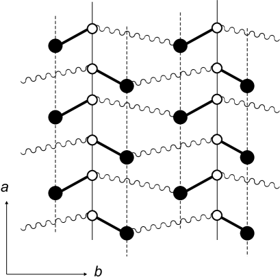
Figure 1: Magnetic model of BIPNNBNO crystal. The black (white) circles denote spins S=1 (s=1/2).

Each of the molecules includes three s=1/2 spins (see Fig. 2) with intramolecular ferromagnetic $J_{F}$ and antiferromagnetic $J_{AF}$ interactions. The magnitude of $|J_{F}|\sim 300$ K is very large, and two spins coupled ferromagnetically behave as a S - 1 moiety. Ferrimagnetic chains are stretched along the b-axis. There are two kinds of antiferromagnetic interchain interactions along the a-axis. One is between the s-1/2 spins, which connects the nearest neighboring chains. The other is between S-1 species, which connects the next nearest neighboring chains and introduces spin frustration.

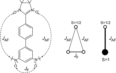
Figure 2: Molecular structure of BIPNNBNO and the elementary magnetic cell at $J_{\textrm{F}}\gg|J_{\textrm{AF}}|$.

The puzzle is following. It is well known that a low-energy physics of an isolated ferrimagnetic (S,s) chain corresponds to a gapless (S-s) ferromagnet Brehmer1997 . Quite predictably one might expect an appearance of an ordered state with fluctuations in the form of spin waves near the classical state. However, measurements of magnetization shows that an opening of a gap by analogy with the Haldane chain is likely scenario. Such a behavior is a manifestation of non-Lieb-Mattis type ferrimagnetism Sakai2011 . Namely, the magnetization measured at 400 mK is nearly zero below 4.5 T, increases rapidly above 4.5 T and exhibits a broad 1/3 plateau and a narrow 2/3 one at 7-23 T and around 26 T, respectively. Above 29 T, the magnetization is completely saturated Goto2003 .

The purpose of the paper is to investigate the magnetization process. The problem is complicated by a lack of reliable information about intra- and interchain exchange interactions. So, before studying of the 2D ferrimagnetic system BIPNNBNO we develop a simple quantum mechanical approach that models a magnetization process of the ferrimagnetic chain (1,1/2). The treatment agrees qualitatively with a predictions of the theory for quantum spin chains Oshikawa1997 and provides reasonable estimations of the exchange intrachain couplings. In addition, it captures a peculiarity of a magnetization process in the prototype 2D material, i.e. an appearance of the intermediate 2/3 plateau. Given these estimations we examine the magnetization process in BIPNNBNO by analyzing exact diagonalization (ED) calculations for a finite clusters of size $N=32$ and $N=40$. A main conclusion to be drawn from these calculations that an emergence of the anomalous singlet plateau is a consequence of the frustrating interchain interaction.

Two different mechanisms of formation of the plateau may be likely candidates: a generalization of Haldane s conjecture to the weakly coupled ferrimagnetic chains, and a valence-bond (dimerized) type ground state in the strong-coupling limit. To determine what of these scenarios is relevant we develop low-energy effective theories for the 4-legs spin tube, which forms a minimal setup including the interchain couplings. In the regime of weakly coupled spin tube legs we apply abelian bosonization technique. The opposite limit of a strong-ring interaction is analyzed in terms of an effective Heisenberg XXZ model where the intrachain coupling is perturbatively taken into account. Our analytical treatment shows that only the first approach confirms an important role of frustration in stabilization of the singlet phase.

Note that a study of spin tubes is of interest by itself because both of frustration and quantum fluctuation are strong Sakai2010 . Our model is directly related with the compound BIPNNBNO, but the main results are expected to apply to other frustrated spin tubes as well. Recently, it has been reported that the experimental candidate for the four-leg spin tube, Cu₂Cl₄$\cdot$D₈C₄SO₂, is available Zheludev2008 .

The paper is organized as follows: In Sec. II we consider a magnetization process in the ferrimagnetic chain ($1,1/2$). In Sec. III we discuss results of magnetization process in two-dimensional ferrimagnetic system obtained via the exact diagonalization method on a finite cluster. In Sec. IV we derive effective low-energy spin-1/2 Hamiltonian. A bosonisation study of the spin tube is carried out in Sec. V. A discussion of these results is relegated to the Conclusion part.

II Magnetization of an isolated ferrimagnetic chain

The issue that we address below is whether a calculation for an isolated ferrimagnetic chain partially reproduces features of the magnetization curve observed in the BIPNNBNO crystal. We demonstrate that both the 1/3 plateau and the 2/3 plateau can be recovered within a simple quantum mechanical analysis of a magnetization process of an isolated quantum $(1,1/2)$ ferrimagnetic chain under an applied magnetic field. This enables to estimate the intrachain exchange parameters $J_{AF}$ and $J_{1}$.

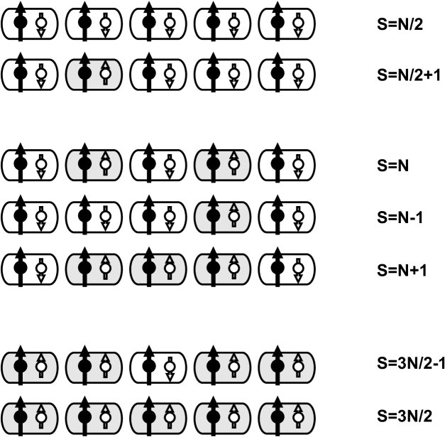
Figure 3: Schematic picture of states of the ferrimagnetic chain used in construction of a magnetization curve. Excited blocks are marked by the gray shadow.

We start from the values of the critical fields derived from the ED data Sakai1991

$$\left\{\begin{array}[]{ccc}B_{1}&=&\left.\frac{\partial\varepsilon}{\partial m}\right|_{m\to 1/3+0}\approx E(N/2+1)-E(N/2),\\ B_{2}&=&\left.\frac{\partial\varepsilon}{\partial m}\right|_{m\to 2/3-0}\approx E(N)-E(N-1),\\ B_{3}&=&\left.\frac{\partial\varepsilon}{\partial m}\right|_{m\to 2/3+0}\approx E(N+1)-E(N),\\ B_{\textrm{sat}}&=&\left.\frac{\partial\varepsilon}{\partial m}\right|_{m\to 1-0}\approx E(3N/2)-E(3N/2-1),\end{array}\right.$$ (1)

where $\varepsilon$, $m$ are the energy and the magnetization per an elementary cell of the $(1,1/2)$ ferrimagnetic chain, $N$ is a number of the elementary cells.

To estimate the energies $E(S)$ in the right-hand side of Eqs.(1), where $S$ is a total spin of the chain, we use the Hamiltonian of the one-dimensional quantum ($1$,$1/2$) ferrimagnet

$$\mathcal{\hat{H}}_{\textrm{c}}=J_{AF}\sum\limits_{i=1}^{N}\vec{S}_{1i}\vec{s}_{2i}+J_{1}\sum\limits_{i=1}^{N}\vec{s}_{2i}\vec{S}_{1i+1}\;(S_{1}=1,\;s_{2}=1/2),$$ (2)

and construct the required quantum states $|SM\rangle$ with the given quantum numbers of the total spin $S$ and its $z$-projection $M$.

We suppose that the $1/3$ magnetization plateau corresponds to the ground state of the ($1$,$1/2$) ferrimagnetic chain with $S=N/2$. The wave function of the polarized state is given by

$$|N/2,N/2\rangle=\prod_{i=1}^{N}\left|\left(1\frac{1}{2}\right)\frac{1}{2}\frac{1}{2}\right\rangle_{i},$$ (3)

and presents a direct product of the spin states of the magnetic elementary cells (1,1/2) [see Fig. 3]. The corresponding energy eigenvalue equals to

$$E(N/2)=-J_{AF}N-\frac{1}{9}J_{1}N.$$ (4)

With an increasing of a magnetic field the ground state (3) is destroying and the state with $S=N/2+1$ stabilizes. A low-lying excitation may be qualitatively considered as a forming of one triplet bond. The trial new wave function is

$$|N/2+1,N/2+1\rangle=\frac{1}{\sqrt{N}}\sum_{k=1}^{N}\left[\prod_{i(\not=k)=1}^{N}\left|\left(1\frac{1}{2}\right)\frac{1}{2}\frac{1}{2}\right\rangle_{i}\right]\left|\left(1\frac{1}{2}\right)\frac{3}{2}\frac{3}{2}\right\rangle_{k}=\sum_{k=1}^{N}\alpha_{k}\Psi_{k}.$$ (5)

It is composed from all arrangements of the excited block within the chain taken with equal weights $\alpha_{k}$.

By introducing the state and calculating the matrix element

$$\langle\Psi_{k}|\mathcal{\hat{H}}_{\textrm{c}}|\Psi_{k^{\prime}}\rangle=\left[E(N/2)+\frac{3}{2}J_{AF}+\frac{7}{18}J_{1}\right]\delta_{kk^{{}^{\prime}}}-\frac{1}{3}J_{1}\delta_{k,k^{\prime}\pm 1}$$ (6)

one obtains the relationship for the coefficients $\alpha_{k}$

$$-\frac{1}{3}J_{1}\alpha_{k-1}+\left[E(N/2)+\frac{3}{2}J_{AF}+\frac{7}{18}J_{1}-E(N/2+1)\right]\alpha_{k}-\frac{1}{3}J_{1}\alpha_{k+1}=0,$$ (7)

which is tantamount to

$$E(N/2+1)=E(N/2)+\frac{3}{2}J_{AF}+\frac{7}{18}J_{1}-\frac{1}{3}J_{1}\left(\frac{\alpha_{k-1}}{\alpha_{k}}+\frac{\alpha_{k+1}}{\alpha_{k}}\right).$$ (8)

This expression includes two independent variational parameters $\alpha_{k-1}/{\alpha_{k}}$ and $\alpha_{k+1}/{\alpha_{k}}$. The minimal value

$$E_{\textrm{min}}(N/2+1)=E(N/2)+\frac{3}{2}J_{AF}-\frac{5}{18}J_{1}$$ (9)

is reached provided $\alpha_{k-1}/{\alpha_{k}}=\alpha_{k+1}/{\alpha_{k}}=1$. This yields the critical magnetic field $B_{1}$ destroying the $1/3$ plateau

$$B_{1}=\frac{3}{2}J_{AF}-\frac{5}{18}J_{1}.$$ (10)

To find the critical fields $B_{2}$ and $B_{3}$ of the beginning and the end of the 2/3 plateau, respectively, we construct the trial states

$$|N,N\rangle=\prod_{i=1}^{N/2}\left|\left(1\frac{1}{2}\right)\frac{1}{2}\frac{1}{2}\right\rangle_{2i-1}\left|\left(1\frac{1}{2}\right)\frac{3}{2}\frac{3}{2}\right\rangle_{2i},$$ (11)

$$|N-1,N-1\rangle=\frac{1}{\sqrt{N}}\sum_{k=1}^{N/2}\left[\prod_{i=1}^{k-1}\left|\left(1\frac{1}{2}\right)\frac{1}{2}\frac{1}{2}\right\rangle_{2i-1}\left|\left(1\frac{1}{2}\right)\frac{3}{2}\frac{3}{2}\right\rangle_{2i}\right]$$

$$\times\left|\left(1\frac{1}{2}\right)\frac{1}{2}\frac{1}{2}\right\rangle_{2k-1}\left|\left(1\frac{1}{2}\right)\frac{1}{2}\frac{1}{2}\right\rangle_{2k}\left[\prod_{i=k+1}^{N/2}\left|\left(1\frac{1}{2}\right)\frac{1}{2}\frac{1}{2}\right\rangle_{2i-1}\left|\left(1\frac{1}{2}\right)\frac{3}{2}\frac{3}{2}\right\rangle_{2i}\right],$$ (12)

$$|N+1,N+1\rangle=\frac{1}{\sqrt{N}}\sum_{k=1}^{N/2}\left[\prod_{i=1}^{k-1}\left|\left(1\frac{1}{2}\right)\frac{1}{2}\frac{1}{2}\right\rangle_{2i-1}\left|\left(1\frac{1}{2}\right)\frac{3}{2}\frac{3}{2}\right\rangle_{2i}\right]$$

$$\times\left|\left(1\frac{1}{2}\right)\frac{3}{2}\frac{3}{2}\right\rangle_{2k-1}\left|\left(1\frac{1}{2}\right)\frac{3}{2}\frac{3}{2}\right\rangle_{2k}\left[\prod_{i=k+1}^{N/2}\left|\left(1\frac{1}{2}\right)\frac{1}{2}\frac{1}{2}\right\rangle_{2i-1}\left|\left(1\frac{1}{2}\right)\frac{3}{2}\frac{3}{2}\right\rangle_{2i}\right],$$ (13)

which are schematically shown in Fig. 3.

By the same manner we obtain

$$B_{2}=\frac{3}{2}J_{AF}+\frac{7}{18}J_{1},\quad B_{3}=\frac{3}{2}J_{AF}+\frac{5}{6}J_{1}.$$ (14)

The saturation field $B_{\textrm{sat}}$ is determined with an aid of the trial wave functions

$$|3N/2,3N/2\rangle=\prod_{i=1}^{N}\left|\left(1\frac{1}{2}\right)\frac{3}{2}\frac{3}{2}\right\rangle_{i},$$ (15)

$$|3N/2-1,3N/2-1\rangle=\frac{1}{\sqrt{N}}\sum_{k=1}^{N}\left[\prod_{i(\not=k)=1}^{N}\left|\left(1\frac{1}{2}\right)\frac{3}{2}\frac{3}{2}\right\rangle_{i}\right]\left|\left(1\frac{1}{2}\right)\frac{1}{2}\frac{1}{2}\right\rangle_{k}$$ (16)

that results in

$$B_{\textrm{sat}}=\frac{3}{2}J_{AF}+\frac{3}{2}J_{1}.$$ (17)

Given the experimental estimations for the 2D BIPNNBNO system, $B_{1}\sim 31\,K$, $B_{2}\approx B_{3}\sim 35\,K$, and $B_{\textrm{sat}}=39\,K$, we obtain from Eqs.(10,17) the values of the intrachain exchange couplings, $J_{AF}\approx 21\,K$ and $J_{1}\approx 3.5\,K$. By substituting them into Eq.(14) we get the critical fields of the 2/3 plateau, $B_{2}\approx 32.8\,K$ ($24.4\,T$) and $B_{3}\approx 34.4\,K$ ($25.6\,T$). A qualitative behavior of the ferrimagnetic chain magnetization curve built from these reference points is depicted in Fig. 4. We emphasize especially that an emergence of the intermediate 2/3 plateau is not related with interchain frustration effects.

Figure 4: Qualitative magnetization curve of the ferrimagnetic $(1,1/2)$ chain.

III Magnetization: Exact Diagonalization

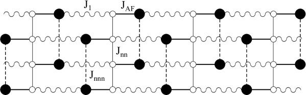
Figure 5: Cluster of $N=32$ sites used in the exact diagonalization. The fixed exchange couplings are $J_{AF}=21K$, $J_{1}=3.5K$, $J_{\textrm{nn}}=0.5J_{1}=1.75K$.

In order to understand a role of the interchain couplings the magnetization process of the BIPNNBNO ferrimagnet was examined by the variant of a numerical diagonalization method with conservation of a total cluster spin Sinitsyn2007 ; Bostrem2010 .

The model Hamiltonian is given by

$$\mathcal{\hat{H}}_{\textrm{clust}}=J_{AF}\sum_{ij}{\vec{S}}_{i}{\vec{s}}_{j}+J_{1}\sum_{ij}{\vec{S}}_{i}{\vec{s}}_{j}+J_{\textrm{nn}}\sum_{ij}{\vec{s}}_{i}{\vec{s}}_{j}+J_{\textrm{nnn}}\sum_{ij}{\vec{S}}_{i}{\vec{S}}_{j},$$ (18)

where $\vec{S}_{i}$ ($\vec{s}_{i}$) denotes spin-1 (spin-1/2) operator at site $i$. The sublattices and the network of the antiferromagnetic interactions, $J_{AF}$, $J_{1}$, $J_{\textrm{nn}}$ and $J_{\textrm{nnn}}$, are shown in Fig. 5. We perform calculation of the N-step magnetization curve for the N=32 cluster depicted in the same Figure. The intrachain parameters, $J_{AF}$ and $J_{1}$, have been estimated in the previous Section whereas the interchain ones, $J_{\textrm{nn}}$ and $J_{\textrm{nnn}}$, are assumed to be less than $J_{1}$. The open boundary conditions are used for the numerical calculations.

The magnetization process is compared with the results of the model of non-interacting (1,1/2) ferrimagnetic chains. A standard way to build magnetization curve at $T=0$ is to define the lowest energy $E(N,M)$ of the Hamiltonian (2) in the subspace where $\sum_{j=1}^{N}\left(S^{z}_{j}+s^{z}_{j}\right)=M$ for a finite system of $N$ elementary $(S,s)$ blocks. Applying a magnetic field $B$ leads to a Zeeman splitting of the energy levels, and therefore level crossing occurs on increasing the field. These level crossing correspond to jumps in the magnetization until the fully polarized state is reached at a certain value of the magnetic field. The magnetization of four independent chains is then derived from

$$m=4M/N,\quad M=\textrm{max}\left[M|E(N,M+1)-E(N,M)>B\right],$$ (19)

which gives a step curve.

Figure 6: Magnetization curve for the 32-site cluster. The exchange couplings are taken as $J_{AF}=21K$, $J_{1}=3.5K$, $J_{\textrm{nn}}=0.5J_{1}$, and $J_{\textrm{nnn}}=0$ (no frustration). The dotted line marks a calculation via the model of non-interacting $(1,1/2)$ chains.

Figure 7: Magnetization curve for the 32-site cluster. The exchange couplings are taken as $J_{AF}=21K$, $J_{1}=3.5K$, $J_{\textrm{nn}}=0.5J_{1}$, $J_{\textrm{nnn}}=0.075J_{1}$. The dotted line marks a calculation via the model of non-interacting $(1,1/2)$ chains.

An importance of the frustrating coupling is seen from comparison of two magnetization curves displayed in Figs. 6, 7. They correspond to no frustration case and a pronounced frustrating coupling, respectively. The magnetization curves exhibit several interesting features. For instance, the magnetization behavior in higher magnetic fields ($B>B_{1}$) is well reproduced within the model of non-interacting ferrimagnetic chains. Another remarkable feature revealed by Figs. 6, 7 that the singlet ground state plateau emerges at non-zero frustration interaction whereas the narrow $2/3$ plateau appears regardless of the frustration. We numerically found that the width $\Delta_{S}$ of the singlet plateau scales almost linearly with a $J_{\textrm{nnn}}$ value (Fig. 8). To check into the case of the dependence we repeat cacluations on a cluster of larger size, $N=40$, with the same set of parameters that support the finding. The observation points out that the zero magnetization plateau has a quantum origin with a crucial role of frustration which destroys a long-range order and drives the system into the singlet phase. Below, we address analytically the issue in the regimes of strong and weak interchain couplings.

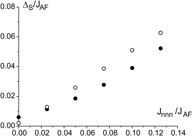
Figure 8: Value of the singlet plateau $\Delta_{S}$ as a function of the frustrating coupling $J_{\textrm{nnn}}$ obtained on a cluster of size $N=32$ (black circles) and $N=40$ (white circles).

IV A formation of the singlet plateau

In low-dimensional Heisenberg systems frustrating couplings can drive transitions to gapfull quantum states, where local singlets form a ground state. These quantum gapped phases may have long-ranged singlet order (valence bond state), or realize a resonating valence band spin liquid. In last case, a ground state is a coherent superposition of all lattice-coverings by local singlets Misguich2005 .

To recognize features of these phases in the ED results we undertake analytical treatments of the four-legs spin tube shown in Fig. 9. The new system is infinite along the $b$-axis, and periodic with the 4-site period along the $a$-axis. The tube forms a minimal setup including the interchain nearest- and next-to-nearest neighbor couplings and contains the same number of ferrimagnetic chains parallel to the b-axis as the clusters in the ED study. As we demonstrate below, the simplified model elucidates an important role of frustration in stabilization of the singlet phase.

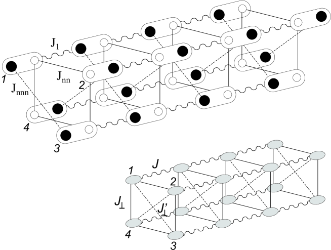
Figure 9: 4-leg spin tube structure used in the limit of strong ring coupling (up) and in the case of weakly interacting chains (below). The black (white) circles mean spin-1 (spin-1/2) sites. The gray circles denote renormalized spin-1/2 blocks.

The singlet phase may arise in the limit of strong ring coupling $J_{\textrm{nn}}$, $J_{\textrm{nnn}}\gg J_{1}$. In this case, the problem can be analyzed in terms of Heisenberg XXZ model similar to ladders in a magnetic field Mila1998 . The opposite limit ($J_{1}\gg J_{\textrm{nn}}$, $J_{\textrm{nnn}}$) results in a scenario of weakly interacting chains. Based on a block renormalization procedure the original system is then mapped onto the model of a spin tube with four ferromagnetic spin-1/2 legs. We mention that the ground state properties of two-leg spin ladders with ferromagnetic intrachain coupling and antiferromagnetic interchain couplings have been discussed in Refs. Kolezhuk1996 ; Roji1996 in an absence of an external field. A magnetization process of those spin ladders with an even number of legs (2 and 4) has been studied in Ref. Wiessner1999 in the regime of weak ferromagnetic coupling along the legs and strong antiferromagnetic coupling along the rungs.

An appearance of the singlet phase in the frustrated spin tube with four weakly coupled ferromagnetic spin-1/2 legs can be studied through the bosonization technique which proves effectiveness for quasi-one-dimensional spin-one-half systems. To the best of our knowledge, the system has never been previously reported, however our further analysis follows closely to that of given in Ref. Kim1999 , where 4-legs spin tube with antiferromagnetic chains and a specific form of diagonal rung interactions (but with no frustration) has been treated. Note as well that spin ladders with ferromagnetic and ferrimagnetic legs are much less studied Japaridze2007 ; Aristov2004 by the bosonization approach in comparison with ladder systems with antiferromagnetic legs. The main problem arising here is that the formalism is well defined only if there is an easy-plane exchange anisotropy. In this regard, we note that measurements of the angular dependence of the ESR linewidth for the BIPNNBNO system showed that the largest linewidth was observed for the field direction perpendicular to the ab plane Kanzawa2006 . Due to the theoretical consideration by Oshikawa and AffleckOshikawa2002 a critical regime of XY-anisotropy is expected in the compound. In addition we point out that the ED algorithm invoked in the previous Section enables to treat clusters of sufficiently large sizes due to use of the rotational $SU(2)$ symmetry. The latter is broken by the anisotropy whose role in a singlet gap formation is a subject of future ED studies.

IV.1 Spin tube: weakly interacting rings and a model of a single XXZ chain

We study the Hamiltonian of the spin tube (see Fig. 9)

$$\mathcal{H}=\sum_{n=1}^{N}H^{\textrm{ring}}_{n}+J_{1}\sum_{n=1}^{N}\left(\textbf{S}_{n,1}\textbf{s}_{n+1,1}+\textbf{s}_{n,2}\textbf{S}_{n+1,2}+\textbf{S}_{n,3}\textbf{s}_{n+1,3}+\textbf{s}_{n,4}\textbf{S}_{n+1,4}\right)-B\sum_{n=1}^{N}\sum_{i=1}^{4}\left(S^{z}_{n,i}+s^{z}_{n,i}\right),$$ (20)

where the Hamiltonian of the separate ring is

$$H^{\textrm{ring}}_{n}=J_{\textrm{nn}}\left(\textbf{s}_{n,1}\textbf{s}_{n,2}+\textbf{s}_{n,2}\textbf{s}_{n,3}+\textbf{s}_{n,3}\textbf{s}_{n,4}+\textbf{s}_{n,4}\textbf{s}_{n,1}\right)+J_{\textrm{nnn}}\sum_{n=1}^{N}\left(\textbf{S}_{n,1}\textbf{S}_{n,3}+\textbf{S}_{n,2}\textbf{S}_{n,4}\right).$$

Here, $S=1$ and $s=1/2$, $n$ is the index of the ring, $N$ is the total number of rings, and the index $i$ marks the (1,1/2) blocks inside the rings. Periodic boundary conditions along the tube direction are imposed. In our model it is suggested that $J_{\textrm{nn}}$, $J_{\textrm{nnn}}\gg J_{1}$.

In the limit $J_{1}=0$ the system decouples into a collection of nonineracting rings. At zero magnetic field the singlet and triplet states

$$|\psi_{0}\rangle=-\frac{\sqrt{3}}{2}|00;00\rangle+\frac{1}{2}|11;00\rangle,$$

$$|\psi_{1}\rangle=\frac{1}{\sqrt{2}}|01;11\rangle+\frac{1}{\sqrt{2}}|10;11\rangle$$ (21)

have the lowest energies $E_{0}=-2J_{\textrm{nn}}/9+8J_{\textrm{nnn}}/9$ and $E_{1}=-J_{\textrm{nn}}/9+8J_{\textrm{nnn}}/9$, respectively. The states of the ring $|S_{12}S_{34};SM\rangle$ are obtained via the common rule of addition of moments, where $S_{12}$ ($S_{34}$) is spin of dimer composed of the spins of the 1 and 2 (3 and 4) blocks. The singlet and triplet states of the ring that enter into (21) are given in Appendix A.

Upon increasing the magnetic field a transition between the singlet and triplet states occurs at $B=J_{\textrm{nn}}/9$ and the the total magnetization jumps abruptly from zero to $M=N$.

At non-zero ring coupling the sharp transition is broadened and starts from a critical value $B_{0}$. To find the field we derive the XXZ spin chain Hamiltonian by we using the standard approach that is analogous to study of spin-1/2 ladder with strong rung exchange Mila1998 .

The Hamiltonian (20) is splitted into two parts

$$\mathcal{H}=\mathcal{H}_{0}+\mathcal{H}_{1}.$$

$$\mathcal{H}_{0}=\sum_{n=1}^{N}H^{\textrm{ring}}_{n}-B_{c}\sum_{i=1}^{4}\sum_{n=1}^{N}\left(S^{z}_{in}+s^{z}_{in}\right),$$

$$\mathcal{H}_{1}=J_{1}\sum_{n=1}^{N}\left[\textbf{S}_{n,1}\textbf{s}_{n+1,1}+\textbf{s}_{n,2}\textbf{S}_{n+1,2}+\textbf{S}_{n,3}\textbf{s}_{n+1,3}+\textbf{s}_{n,4}\textbf{S}_{n+1,4}\right]-\left(B-B_{c}\right)\sum_{i=1}^{4}\sum_{n=1}^{N}(S^{z}_{in}+s^{z}_{in}),$$

where $B_{c}=E_{1}-E_{0}$. The $\mathcal{H}_{1}$ lifts the $2^{N}$-fold degeneracy of the ground state of the Hamiltonian $\mathcal{H}_{0}$ . The later can be either in the state $|\psi_{0}\rangle$ or $|\psi_{1}\rangle$. By using the standard many body perturbation theory Fulde the effective Hamiltonian can be derived

$$\mathcal{H}_{\textrm{eff}}=J^{\textrm{eff}}_{xy}\sum_{n=1}^{N}\left(\tilde{S}^{x}_{n}\tilde{S}^{x}_{n+1}+\tilde{S}^{y}_{n}\tilde{S}^{y}_{n+1}\right)+J^{\textrm{eff}}_{z}\sum_{n=1}^{N}\tilde{S}^{z}_{n}\tilde{S}^{z}_{n+1}-H^{\textrm{eff}}_{z}\sum_{n=1}^{N}\tilde{S}^{z}_{n},$$ (22)

where $J^{\textrm{eff}}_{xy}=-16J_{1}/27$, $J^{\textrm{eff}}_{z}=-J_{1}/9$ and $B^{\textrm{eff}}_{z}=J_{1}/9+B-B_{c}$.

To get the expression the pseudo-spin $\tilde{S}_{i}=1/2$ operators that act on the states $|\psi_{0}\rangle$ and $|\psi_{1}\rangle$ are introduced

$$\tilde{S}^{z}_{n}|\psi_{0}\rangle_{n}=-\frac{1}{2}|\psi_{0}\rangle_{n},\qquad\tilde{S}^{z}_{n}|\psi_{1}\rangle_{n}=\frac{1}{2}|\psi_{1}\rangle_{n},$$

$$\tilde{S}^{+}_{n}|\psi_{0}\rangle_{n}=|\psi_{1}\rangle_{n},\qquad\tilde{S}^{+}_{n}|\psi_{1}\rangle_{n}=0,$$

$$\tilde{S}^{-}_{n}|\psi_{0}\rangle_{n}=0,\qquad\tilde{S}^{-}_{n}|\psi_{1}\rangle_{n}=|\psi_{0}\rangle_{n}.$$ (23)

The starting spin-1 operators and the pseudo-spin operators in the restricted space are related by

$$S^{z}_{in}=\frac{1}{6}+\frac{1}{3}{\tilde{S}}^{z}_{n},$$

$$S^{+}_{in}=(-1)^{i-1}\frac{4}{3\sqrt{3}}{\tilde{S}}^{+}_{n},\qquad S^{-}_{in}=(-1)^{i-1}\frac{4}{3\sqrt{3}}{\tilde{S}}^{-}_{n}.$$ (24)

The corresponding map for the spin-1/2 operators is

$$s^{z}_{in}=-\frac{1}{24}-\frac{1}{12}{\tilde{S}}^{z}_{n},$$

$$s^{+}_{in}=\frac{(-1)^{i}}{3\sqrt{3}}{\tilde{S}}^{+}_{n},\qquad s^{-}_{in}=\frac{(-1)^{i}}{3\sqrt{3}}{\tilde{S}}^{-}_{n}.$$ (25)

The Jordan-Wigner transformation maps the Hamiltonian (22) onto a system of interacting spinless fermions

$$\mathcal{H}_{sf}=t\sum_{n=1}^{N}\left(c^{+}_{i}c_{i+1}+c^{+}_{i+1}c_{i}\right)+V\sum_{n=1}^{N}n_{i}n_{i+1}-\mu\sum_{n=1}^{N}n_{i},$$ (26)

where $t=J^{\textrm{eff}}_{xy}/2$, $V=J^{\textrm{eff}}_{z}$ and $\mu=J^{\textrm{eff}}_{z}+B^{\textrm{eff}}_{z}$.

The lowest critical field $B_{0}$ corresponds to that value of the chemical potential $\mu$ for which the band of spinless fermions starts to fill up. This yields the condition $\mu=-2t$ and leads to the result

$$B_{0}=\frac{1}{9}J_{\textrm{nn}}+\frac{16}{27}J_{1}.$$ (27)

The critical value involves no frustration parameter $J_{\textrm{nnn}}$ that is clearly contrary to the ED results.

A similar analysis can be carried out for the saturation field. The details of the calculations are relegated to Appendix B.

IV.2 Spin tube: a model of weakly interacting ferromagnetic legs and abelian bosonization

To apply the bosonization we should map the initial system, consisting of two sorts of spins, spin-1/2 and spin-1, to the spin-1/2 system by using the quantum renormalization group (QRG) in real space based on the block renormalization procedure pfeuty . To exploit the real-space QRG technique one divide the spin lattice into small blocks, namely, the intrachain dimers (1,1/2), and obtains the lowest energy states $\left\{\left|\alpha\right\rangle\right\}$ of each isolated block. The effect of inter-block interactions is then taken into account by constructing an effective Hamiltonian $H_{\textrm{eff}}$ which now acts on a smaller Hilbert space embedded in the original one. In this new Hilbert space each of the former blocks is treated as a single site. The effective Hamiltonians $H_{\textrm{eff}}=Q^{\dagger}HQ$ is constructed via the projection operator $Q=\prod\limits_{i=1}^{N}Q_{i}$ with $Q_{i}=\sum\limits_{\alpha=1}^{m}\left|\alpha\right\rangle\left\langle\alpha\right|$ of each $i$-th block where $m$ is the number of low energy states that are kept and $N$ is a number of lattice cells.

We hold the lowest doublet $S-1/2$ to find an effective low-energy Hamiltonian. The higher energy $S-3/2$ states are neglected. One can check that the reduced matrix elements are ($S_{1}=1$, $s_{2}=1/2$)

$$\langle 1\,1/2;1/2||S_{1}||1\,1/2;1/2\rangle=2\sqrt{\frac{2}{3}},$$

$$\langle 1\,1/2;1/2||s_{2}||1\,1/2;1/2>=-\frac{1}{\sqrt{6}}.$$

Therefore the effective spin-1/2 operators of the renormalized chain are

$$Q_{i}^{\dagger}\vec{S}_{1i}Q_{i}=\frac{4}{3}\vec{S}_{i},\;Q_{i}^{\dagger}\vec{s}_{2i}Q_{i}=-\frac{1}{3}\vec{S}_{i}\qquad(S=1/2).$$ (28)

The renormalized Hamiltonian of the intrachain interactions corresponds to the ferromagnetic Heisenberg spin-1/2 model with the exchange coupling $J=-4J_{1}/9$ (Fig. 9). The interchain interactions between the nearest neighbors, spins -1/2, and next to the nearest neighbors, spins -1, are renormalized as $J_{\perp}=J_{\textrm{nn}}/9$ and $J^{{}^{\prime}}_{\perp}=16J_{\textrm{nnn}}/9$, respectively.

Consider a four-legs spin tube consisting of spin-$1/2$ chains. The Hamiltonian of the system is

$$\mathcal{{\hat{H}}}_{\textrm{tube}}=\sum_{\lambda=1}^{4}\mathcal{{\hat{H}}}_{\lambda}+\mathcal{{\hat{H}}}^{\perp}_{12}+\mathcal{{\hat{H}}}^{\perp}_{23}+\mathcal{{\hat{H}}}^{\perp}_{34}+\mathcal{{\hat{H}}}^{\perp}_{14}+\mathcal{{\hat{H}}}^{{}^{\prime}\,\perp}_{13}+\mathcal{{\hat{H}}}^{{}^{\prime}\,\perp}_{24}.$$ (29)

The spins along the chains are coupled ferromagnetically, the Hamiltonian for the separate $\lambda$-th chain is

$$\mathcal{{\hat{H}}}_{\lambda}=-J^{xy}\sum_{i=1}^{N}\left(S^{x}_{\lambda,j}S^{x}_{\lambda,j+1}+S^{y}_{\lambda,j}S^{y}_{\lambda,j+1}\right)-J^{z}\sum_{i=1}^{N}S^{z}_{\lambda,j}S^{z}_{\lambda,j+1},$$

where $S^{x,y,z}_{\lambda,j}$ are the spin S=1/2 operators at the $j$th site, the intraleg coupling is ferromagnetic, $J>0$.

The interaction parts are given by

$$\mathcal{{\hat{H}}}^{\perp}_{\lambda\lambda^{\prime}}=J^{xy}_{\perp,\lambda\lambda^{\prime}}\sum_{j=1}^{N}\left(S^{x}_{\lambda,j}S^{x}_{\lambda^{\prime},j}+S^{y}_{\lambda,j}S^{y}_{\lambda^{\prime},j}\right)+J^{z}_{\perp,\lambda\lambda^{\prime}}\sum_{i=1}^{N}S^{z}_{\lambda,j}S^{z}_{\lambda,j},$$ (30)

$$\mathcal{{\hat{H}}}^{{}^{\prime}\,\perp}_{\lambda\lambda^{\prime}}=J^{{}^{\prime}\,xy}_{\perp,\lambda\lambda^{\prime}}\sum_{j=1}^{N}\left(S^{x}_{\lambda,j}S^{x}_{\lambda^{\prime},j}+S^{y}_{\lambda,j}S^{y}_{\lambda^{\prime},j}\right)+J^{{}^{\prime}\,z}_{\perp,\lambda\lambda^{\prime}}\sum_{i=1}^{N}S^{z}_{\lambda,j}S^{z}_{\lambda,j}$$ (31)

and includes the nearest, $J_{\perp}>0$, and the next-to-nearest, $J^{{}^{\prime}}_{\perp}>0$, antiferromagnetic interleg couplings.

The unitary transformation keeping spin commutation relations

$$S^{x,y}_{\lambda,j}\to(-1)^{j}S^{x,y}_{\lambda,j},\quad S^{z}_{\lambda,j}\to S^{z}_{\lambda,j}$$

maps the Hamiltonian (29) to the Hamiltonian with antiferromagnetic legs. It changes $J^{xy}\to-J^{xy}$ and $J^{z}\to J^{z}$, and the ferromagnetic isotropic point is $\Delta=J^{z}/J^{xy}=-1$ in the Hamiltonian with the antiferromagnetic legs.

Following the general procedure of transforming a spin model to an effective model of continuum field, we convert the spin Hamiltonian of the spin tube with antiferromagnetic legs to a Hamiltonian of spinless fermions using Jordan-Wigner transformation, then map it to a modified Luttinger model. The bosonic expressions for spin operators are

$$S^{+}_{\lambda}(x)=\frac{S^{+}_{j\lambda}}{a}=\frac{e^{-i\sqrt{\pi}\Theta_{\lambda}}}{\sqrt{2\pi a}}\left[e^{-i(\pi x/a)}+\cos\left(\sqrt{4\pi}\Phi_{\lambda}\right)\right],$$

$$S^{z}_{\lambda}(x)=\frac{S^{z}_{j\lambda}}{a}=\frac{1}{\sqrt{\pi}}\partial_{x}\Phi_{\lambda}+\frac{1}{\pi a}e^{i(\pi x/a)}\sin\left(\sqrt{4\pi}\Phi_{\lambda}\right),$$ (32)

where $\Phi$ and $\Theta$ are the bosonic dual fields, and $x$ is defined on the lattice, $x_{j}=ja$, $a$ is a short-distance cutoff.

The bosonized form of the Hamiltonian of the non-interacting chains is

$$\mathcal{H}_{\lambda}=\frac{u}{2}\int dx\,\left[K\Pi^{2}_{\lambda}+\frac{1}{K}\left(\partial_{x}\Phi_{\lambda}\right)^{2}\right],$$ (33)

where $\Pi_{\lambda}(x)=\partial_{x}\Theta_{\lambda}$ is canonically conjugate momentum to $\Phi_{\lambda}$. The Luttinger liquid parameters are fixed from the Bethe ansatz solution Luther1975

$$K=\frac{\pi}{2(\pi-\arccos\Delta)},\qquad u=J^{xy}\,\frac{\pi\sqrt{1-\Delta^{2}}}{2\arccos\Delta}.$$ (34)

The velocity $u$ vanishes and $K$ diverges for $\Delta=-1$. This corresponds to the ferromagnetic instability point of a single chain.

The interchain interactions (30) between the nearest neighbor chains reads as

$$\mathcal{H}^{\perp}_{\lambda\lambda^{\prime}}=J^{z}_{\perp,\lambda\lambda^{{}^{\prime}}}\int\frac{dx}{\pi}\left(\partial_{x}\Phi_{\lambda}\right)\left(\partial_{x}\Phi_{\lambda^{{}^{\prime}}}\right)+g_{1}\int\frac{dx}{(2\pi a)^{2}}\cos\left(\sqrt{4\pi}(\Phi_{\lambda}+\Phi_{\lambda^{{}^{\prime}}})\right)$$

$$+g_{2}\int\frac{dx}{(2\pi a)^{2}}\cos\left(\sqrt{4\pi}(\Phi_{\lambda}-\Phi_{\lambda^{{}^{\prime}}})\right)+g_{3}\int\frac{dx}{(2\pi a)^{2}}\cos\left(\sqrt{\pi}(\Theta_{\lambda}-\Theta_{\lambda^{{}^{\prime}}})\right)$$

$$+g_{4}\int\frac{dx}{(2\pi a)^{2}}\cos\left(\sqrt{\pi}(\Theta_{\lambda}-\Theta_{\lambda^{{}^{\prime}}})\right)\cos\left(\sqrt{4\pi}(\Phi_{\lambda}+\Phi_{\lambda^{{}^{\prime}}})\right)$$

$$+g_{5}\int\frac{dx}{(2\pi a)^{2}}\cos\left(\sqrt{\pi}(\Theta_{\lambda}-\Theta_{\lambda^{{}^{\prime}}})\right)\cos\left(\sqrt{4\pi}(\Phi_{\lambda}-\Phi_{\lambda^{{}^{\prime}}})\right),$$ (35)

where $g_{1}=-2J^{z}_{\perp,\lambda\lambda^{{}^{\prime}}}$, $g_{2}=2J^{z}_{\perp,\lambda\lambda^{{}^{\prime}}}$, $g_{3}=2\pi J^{xy}_{\perp,\lambda\lambda^{{}^{\prime}}}$, $g_{4}=g_{5}=\pi J^{xy}_{\perp,\lambda\lambda^{{}^{\prime}}}$. The Hamiltonian (31) of the next-to-nearest couplings has a similar form with a formal change $J^{z}_{\perp,\lambda\lambda^{{}^{\prime}}}\to J^{{}^{\prime}\,z}_{\perp,\lambda\lambda^{{}^{\prime}}}$, $g_{1}\to g^{{}^{\prime}}_{1}=-2J^{{}^{\prime}\,z}_{\perp,\lambda\lambda^{{}^{\prime}}}$, $g_{2}\to g^{{}^{\prime}}_{2}=2J^{{}^{\prime}\,z}_{\perp,\lambda\lambda^{{}^{\prime}}}$ etc.

Following the route of Refs.Kim1999 ; Cabra1998 it is convenient to introduce a symmetric mode $\Phi_{s}$ and three antisymmetric ones $\Phi_{a_{1}}$, $\Phi_{a_{2}}$, $\Phi_{a_{3}}$

$$\begin{array}[]{c}\Phi_{s}=\frac{1}{2}\left(\Phi_{1}+\Phi_{2}+\Phi_{3}+\Phi_{4}\right),\\ \Phi_{a_{1}}=\frac{1}{2}\left(\Phi_{1}+\Phi_{2}-\Phi_{3}-\Phi_{4}\right),\\ \Phi_{a_{2}}=\frac{1}{2}\left(\Phi_{1}-\Phi_{2}-\Phi_{3}+\Phi_{4}\right),\\ \Phi_{a_{3}}=\frac{1}{2}\left(\Phi_{1}-\Phi_{2}+\Phi_{3}-\Phi_{4}\right).\end{array}$$ (36)

In terms of the new fields the quadratic part of the Hamiltonian (29) is diagonalized to

$$\mathcal{H}_{0}=\frac{u_{s}}{2}\int dx\,\left[K_{s}\Pi^{2}_{s}+\frac{1}{K_{s}}\left(\partial_{x}\Phi_{s}\right)^{2}\right]+\sum_{i=1}^{3}\frac{u_{a_{i}}}{2}\int dx\,\left[K_{a_{i}}\Pi^{2}_{a_{i}}+\frac{1}{K_{a_{i}}}\left(\partial_{x}\Phi_{a_{i}}\right)^{2}\right]$$ (37)

with

$$u_{s}=u\left(1+\frac{2KJ^{z}_{\perp}}{u\pi}+\frac{KJ^{{}^{\prime}\,z}_{\perp}}{u\pi}\right)^{\frac{1}{2}},\qquad K_{s}=K\left(1+\frac{2KJ^{z}_{\perp}}{u\pi}+\frac{KJ^{{}^{\prime}\,z}_{\perp}}{u\pi}\right)^{-\frac{1}{2}},$$

$$u_{a_{1}}=u_{a_{2}}=u\left(1-\frac{KJ^{{}^{\prime}\,z}_{\perp}}{u\pi}\right)^{\frac{1}{2}},\qquad K_{a_{1}}=K_{a_{2}}=K\left(1-\frac{KJ^{{}^{\prime}\,z}_{\perp}}{u\pi}\right)^{-\frac{1}{2}},$$

$$u_{a_{3}}=u\left(1-\frac{2KJ^{z}_{\perp}}{u\pi}+\frac{KJ^{{}^{\prime}\,z}_{\perp}}{u\pi}\right)^{\frac{1}{2}},\qquad K_{a_{3}}=K\left(1-\frac{2KJ^{z}_{\perp}}{u\pi}+\frac{KJ^{{}^{\prime}\,z}_{\perp}}{u\pi}\right)^{-\frac{1}{2}}.$$ (38)

The relevant and marginally relevant terms of the interchain couplings are given by

$$\mathcal{H}_{\textrm{int}}=2g_{1}\sum_{i=1}^{2}\int\frac{dx}{(2\pi a)^{2}}\cos\left(\sqrt{4\pi}\Phi_{s}\right)\cos\left(\sqrt{4\pi}\Phi_{a_{i}}\right)+2g^{{}^{\prime}}_{1}\int\frac{dx}{(2\pi a)^{2}}\cos\left(\sqrt{4\pi}\Phi_{s}\right)\cos\left(\sqrt{4\pi}\Phi_{a_{3}}\right)$$

$$+2g_{2}\sum_{i=1}^{2}\int\frac{dx}{(2\pi a)^{2}}\cos\left(\sqrt{4\pi}\Phi_{a_{i}}\right)\cos\left(\sqrt{4\pi}\Phi_{a_{3}}\right)+2g^{{}^{\prime}}_{2}\int\frac{dx}{(2\pi a)^{2}}\cos\left(\sqrt{4\pi}\Phi_{a_{1}}\right)\cos\left(\sqrt{4\pi}\Phi_{a_{2}}\right)$$

$$+2g_{3}\sum_{i=1}^{2}\int\frac{dx}{(2\pi a)^{2}}\cos\left(\sqrt{\pi}\Theta_{a_{i}}\right)\cos\left(\sqrt{\pi}\Theta_{a_{3}}\right)+2g^{{}^{\prime}}_{3}\int\frac{dx}{(2\pi a)^{2}}\cos\left(\sqrt{\pi}\Theta_{a_{1}}\right)\cos\left(\sqrt{\pi}\Theta_{a_{2}}\right)$$

$$+g_{4}\int\frac{dx}{(2\pi a)^{2}}\left[\cos\left(\sqrt{\pi}(\Theta_{a_{2}}+\Theta_{a_{3}})\right)\cos\left(\sqrt{4\pi}(\Phi_{s}+\Phi_{a_{1}})\right)\right.$$

$$+\cos\left(\sqrt{\pi}(\Theta_{a_{1}}-\Theta_{a_{3}})\right)\cos\left(\sqrt{4\pi}(\Phi_{s}-\Phi_{a_{2}})\right)+\cos\left(\sqrt{\pi}(\Theta_{a_{2}}-\Theta_{a_{3}})\right)\cos\left(\sqrt{4\pi}(\Phi_{s}-\Phi_{a_{1}})\right)$$

$$\left.+\cos\left(\sqrt{\pi}(\Theta_{a_{1}}+\Theta_{a_{3}})\right)\cos\left(\sqrt{4\pi}(\Phi_{s}+\Phi_{a_{2}})\right)\right]$$

$$+g^{{}^{\prime}}_{4}\int\frac{dx}{(2\pi a)^{2}}\left[\cos\left(\sqrt{\pi}(\Theta_{a_{1}}+\Theta_{a_{2}})\right)\cos\left(\sqrt{4\pi}(\Phi_{s}+\Phi_{a_{3}})\right)\right.$$

$$\left.+\cos\left(\sqrt{\pi}(\Theta_{a_{1}}-\Theta_{a_{2}})\right)\cos\left(\sqrt{4\pi}(\Phi_{s}-\Phi_{a_{3}})\right)\right].$$ (39)

The $g_{5}$ terms are irrelevant and are omitted.

The Hamiltonian (37) describes four independent gapless spin-$1/2$ chains coupled by the interchain interaction in the form of Eq.(39). It is expected that the interleg coupling results in the Haldane gap in the excitation spectrum. Note that in the vicinity of the single chain ferromagnetic instability, $\Delta=-1$, the effective bandwidth collapses, $u\to 0$, and the effect of the interleg couplings becomes crucial. To find a detail behavior of the gap in the phase diagram with antiferromagnetic ($J_{\perp}$, $J^{{}^{\prime}}_{\perp}>0$) interleg coupling and ferromagnetic leg regime ($\Delta<0$) we use the renormalization group analysis.

The RG equations are derived through the standard technique (see Ref.Giamarchi , for example). The result is

$$\frac{dg_{1}}{dl}=\left[2-\left(K_{s}+K_{a_{1}}\right)\right]g_{1},$$

$$\frac{dg^{{}^{\prime}}_{1}}{dl}=\left[2-\left(K_{s}+K_{a_{3}}\right)\right]g^{{}^{\prime}}_{1},$$

$$\frac{dg_{2}}{dl}=\left[2-\left(K_{a_{3}}+K_{a_{1}}\right)\right]g_{2},$$

$$\frac{dg^{{}^{\prime}}_{2}}{dl}=\left[2-2K_{a_{1}}\right]g^{{}^{\prime}}_{2},$$

$$\frac{dg_{3}}{dl}=\left[2-\frac{1}{4}\left(\frac{1}{K_{a_{1}}}+\frac{1}{K_{a_{3}}}\right)\right]g_{3},$$

$$\frac{dg^{{}^{\prime}}_{3}}{dl}=\left[2-\frac{1}{2K_{a_{1}}}\right]g^{{}^{\prime}}_{3},$$

$$\frac{dg_{4}}{dl}=\left[2-\left(K_{s}+K_{a_{1}}+\frac{1}{4K_{a_{1}}}+\frac{1}{4K_{a_{3}}}\right)\right]g_{4},$$

$$\frac{dg^{{}^{\prime}}_{4}}{dl}=\left[2-\left(K_{s}+K_{a_{3}}+\frac{1}{2K_{a_{1}}}\right)\right]g^{{}^{\prime}}_{4},$$

$$\frac{dK_{s}}{dl}=-4g^{2}_{1}\left(\frac{K_{s}}{4\pi u_{s}}\right)^{2}-2{g^{{}^{\prime}}_{1}}^{2}\left(\frac{K_{s}}{4\pi u_{s}}\right)^{2}-2g^{2}_{4}\left(\frac{K_{s}}{4\pi u_{s}}\right)^{2}-{g^{{}^{\prime}}_{4}}^{2}\left(\frac{K_{s}}{4\pi u_{s}}\right)^{2},$$

$$\frac{dK_{a_{1}}}{dl}=-\frac{1}{2}g^{2}_{1}\left(\frac{K_{a_{1}}}{2\pi u_{a_{1}}}\right)^{2}-\frac{1}{2}g^{2}_{2}\left(\frac{K_{a_{1}}}{2\pi u_{a_{1}}}\right)^{2}-\frac{1}{2}{g^{{}^{\prime}}_{2}}^{2}\left(\frac{K_{a_{1}}}{2\pi u_{a_{1}}}\right)^{2}-\frac{1}{4}g^{2}_{4}\left(\frac{K_{a_{1}}}{2\pi u_{a_{1}}}\right)^{2}$$

$$+\frac{1}{2}\left(\frac{g_{3}}{4\pi u_{a_{1}}}\right)^{2}+\frac{1}{2}\left(\frac{g^{{}^{\prime}}_{3}}{4\pi u_{a_{1}}}\right)^{2}+\frac{1}{4}\left(\frac{g_{4}}{4\pi u_{a_{1}}}\right)^{2}+\frac{1}{4}\left(\frac{g^{{}^{\prime}}_{4}}{4\pi u_{a_{1}}}\right)^{2},$$

$$\frac{dK_{a_{3}}}{dl}=-\frac{1}{2}{g^{{}^{\prime}}_{1}}^{2}\left(\frac{K_{a_{3}}}{2\pi u_{a_{3}}}\right)^{2}-g^{2}_{2}\left(\frac{K_{a_{3}}}{2\pi u_{a_{3}}}\right)^{2}-\frac{1}{4}{g^{{}^{\prime}}_{4}}^{2}\left(\frac{K_{a_{3}}}{2\pi u_{a_{3}}}\right)^{2}$$

$$+\left(\frac{g_{3}}{4\pi u_{a_{3}}}\right)^{2}+\frac{1}{2}\left(\frac{g_{4}}{4\pi u_{a_{3}}}\right)^{2}.$$ (40)

One sees that the $g_{1}$ terms are relevant for $K_{s}+K_{a_{1}}<2$; the $g^{{}^{\prime}}_{1}$ term is relevant for $K_{s}+K_{a_{3}}<2$; the $g_{2}$ terms are relevant for $K_{a_{3}}+K_{a_{1}}<2$; the $g^{{}^{\prime}}_{2}$ term is relevant for $K_{a_{1}}<1$; the $g_{3}$ term is relevant for $K^{-1}_{a_{1}}+K^{-1}_{a_{3}}<8$; the $g^{{}^{\prime}}_{3}$ term is relevant for $K_{a_{1}}>1/4$. Despite the $g_{4}$ and $g^{{}^{\prime}}_{4}$ terms are irrelevant they are the most relevant terms which couple the symmetric and antisymmetric modes Kim1999 .

Using the RG equations the behavior of the gap in the whole phase diagram can be established. Following to standard routine, we analyze the effect of the transversal ($J^{xy}_{\perp}$) and the longitudinal ($J^{z}_{\perp}$) parts of the interleg coupling separately.

IV.2.1 Transversal part of the interleg interactions

In this case $J^{xy}_{\perp},J^{{}^{\prime}\,xy}_{\perp}\neq 0$ and $J^{z}_{\perp},J^{{}^{\prime}\,z}_{\perp}=0$, the initial values of the coupling constants are given by $g_{1}(l=0)=g^{{}^{\prime}}_{1}(l=0)=0$, $g_{2}(l=0)=g^{{}^{\prime}}_{2}(l=0)=0$, $g_{3}(l=0)=2\pi J^{xy}_{\perp}$, $g^{{}^{\prime}}_{3}(l=0)=2\pi J^{{}^{\prime}\,xy}_{\perp}$, $g_{4}(l=0)=\pi J^{xy}_{\perp}$ and $g^{{}^{\prime}}_{4}(l=0)=\pi J^{{}^{\prime}\,xy}_{\perp}$. The bare Luttinger parameters are $u_{s}=u$, $u_{a_{1}}=u_{a_{2}}=u_{a_{3}}=u$, and $K_{s}(l=0)=K$, $K_{a_{1}}(l=0)=K_{a_{2}}(l=0)=K_{a_{3}}(l=0)=K$. The term $g_{3}$ is relevant for $-1\leq\Delta\leq 0$ while the $g_{4}$ term is irrelevant. It is easily checked numerically that $g_{3}$, $g^{{}^{\prime}}_{3}$ grow whereas $g_{4}$, $g^{{}^{\prime}}_{4}$ decrease under the RG. It means that $\Theta_{1}$, $\Theta_{2}$, $\Theta_{3}$ are locked in one of the vacuum states ($\Theta_{1}=\Theta_{2}=0$, $\Theta_{3}=\sqrt{\pi}$ or $\Theta_{1}=\Theta_{2}=\sqrt{\pi}$, $\Theta_{3}=0$ provided $J^{xy}_{\perp}>$$J^{{}^{\prime}\,xy}_{\perp}$), fluctuations of the fields $\Theta_{a_{i}}$ ($i=1,2,3$) are completely suppressed. Therefore arbitrary $J^{xy}_{\perp}>J^{{}^{\prime}\,xy}_{\perp}\neq 0$ generate a gap in the antisymmetric modes ($\Theta_{i}$ are pinned, disordered).

After the fluctuations of the fields $\Theta_{i}$ are stopped, the infrared behavior of the symmetric mode is governed by the term of the coupling with the antisymmetric modes

$$\mathcal{\tilde{H}}_{\textrm{int}}=2\tilde{g}_{4}\sum_{i=1}^{2}\int\frac{dx}{(2\pi a)^{2}}\cos(\sqrt{4\pi}\Phi_{s})\cos(\sqrt{4\pi}\Phi_{a_{i}})$$

$$+2\tilde{g}^{{}^{\prime}}_{4}\int\frac{dx}{(2\pi a)^{2}}\cos(\sqrt{4\pi}\Phi_{s})\cos(\sqrt{4\pi}\Phi_{a_{3}}).$$ (41)

where

$$\tilde{g}_{4}=\bar{g}_{4}\langle\cos\left(\sqrt{\pi}[\Theta_{a_{1}}+\Theta_{a_{3}}]\right)\rangle=\bar{g}_{4}\langle\cos\left(\sqrt{\pi}[\Theta_{a_{2}}+\Theta_{a_{3}}]\right)\rangle,$$

$$\tilde{g}^{{}^{\prime}}_{4}=\bar{g}^{{}^{\prime}}_{4}\langle\cos\left(\sqrt{\pi}(\Theta_{a_{1}}+\Theta_{a_{2}})\right)\rangle,$$

and $\bar{g}_{4}$, $\bar{g}^{{}^{\prime}}_{4}$ are renormalized couplings provided $g_{3},g^{{}^{\prime}}_{3}=\mathcal{O}(1)$. Here, the invariance of $\mathcal{\tilde{H}}_{\textrm{int}}$ given by Eq.(39) under $\Theta_{a_{i}}\to-\Theta_{a_{i}}$ yields $\langle\cos\left(\sqrt{\pi}(\Theta_{a_{i}}-\Theta_{a_{j}})\right)\rangle=\langle\cos\left(\sqrt{\pi}(\Theta_{a_{i}}+\Theta_{a_{j}})\right)\rangle$. Despite $e^{i\Phi_{a_{i}}}$ has exponentially decaying correlations due to the $\Theta_{a_{i}}$ are pinned, a scrupulous analysis Kim1999 shows that the effective Hamiltonian for $\Phi_{s}$ presents a standard sine-Gordon Hamiltonian

$$\mathcal{\tilde{H}}_{\textrm{eff}}=\frac{u_{s}}{2}\int dx\,\left[\bar{K}_{s}\Pi^{2}_{s}+\frac{1}{\bar{K}_{s}}\left(\partial_{x}\Phi_{s}\right)^{2}\right]+g\int\frac{dx}{(2\pi a)^{2}}\cos\left(\sqrt{16\pi}\Phi_{s}\right),$$ (42)

where $\bar{K}_{s}$ is a renormalized value of $K$, and $g$ is a new effective coupling constant. From the correlation function $\langle\exp\left[i\sqrt{16\pi}\Phi_{s}(x)\right]\exp\left[i\sqrt{16\pi}\Phi_{s}(y)\right]\rangle=\left(a^{2}/|x-y|^{2}\right)^{4\bar{K}_{s}}$ it follows that the $g$ term has a scale dimension $4\bar{K}_{s}$. Therefore, it is relevant for $\bar{K}_{s}<1/2$, when $\Phi_{s}$ is pinned, i.e. becomes massive Tsvelik .

To summarize, the transversal part of the interleg coupling supports gapped antisymmetric modes, the symmetric sector is gapped at $\bar{K}_{s}<1/2$, and remains gapless at $\bar{K}_{s}>1/2$. The condition $\bar{K}_{s}=1/2$ determines a boundary between the gapless Spin Liquid XY1 phase Shulz , and a generalization of the gapped Rung Singlets phase Vekua2003 for the for-leg spin tube (Fig.10). (Hereinafter, we retain names of phases used in the theory of spin ladders with ferromagnetic legs.) In the last case, spins on the same rungs, or along the shortest diagonals form singlet pairs by a dynamical way.

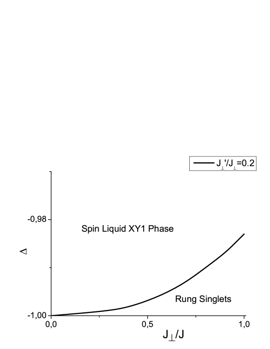
Figure 10: The ground-state phase diagram in the vicinity $\Delta=-1$ of the four-leg tube with transverse coupling between legs.

IV.2.2 Longitudinal part of the interleg interactions

For the case of the longitudinal part of the interleg exchange, $J^{xy}_{\perp},J^{{}^{\prime}\,xy}_{\perp}=0$ and $J^{z}_{\perp},J^{{}^{\prime}\,z}_{\perp}\neq 0$, the bare values of the coupling constants are given by $g_{1}(l=0)=-2J^{z}_{\perp}$, $g^{{}^{\prime}}_{1}(l=0)=-2J^{{}^{\prime}\,z}_{\perp}$, $g_{2}(l=0)=2J^{z}_{\perp}$, $g^{{}^{\prime}}_{2}(l=0)=2J^{{}^{\prime}\,z}_{\perp}$, $g_{3}(l=0)=g^{{}^{\prime}}_{3}(l=0)=0$, and $g_{4}(l=0)=g^{{}^{\prime}}_{4}(l=0)=0$.

Figure 11: The ground-state phase diagram in the vicinity $\Delta=-1$ of the four-leg tube with longitudinal coupling between legs.

The strong-coupling phase diagram in the vicinity of ferromagnetic instability point ($\Delta=-1$ and $J^{z}_{\perp},J^{{}^{\prime}\,z}_{\perp}=0$) obtained in the RG analysis is shown in Fig. 11. In the sector denoted as spin liquid II phaseVekua2003 the $g_{1,2}$, $g^{{}^{\prime}}_{1,2}$ terms are irrelevant. The symmetric and antisymmetric modes remain gapless. In the sector marked as a Haldane phase the terms $g_{1,2}$, $g^{{}^{\prime}}_{1,2}$ are relevant. Since all of the modes are coupled and locked together, both the symmetric and antisymmetric modes are gapped.

The phase of a ferromagnet with antiphase interchain order arises as a result of the ferromagnetic instability with increasing interleg antiferromagnetic coupling. The boundary of the transition into the phase is obtained by studying the velocity renormalization of the corresponding gapless excitations. We mark the transition at $u_{a_{i}}=0$ ($i=1,2,3$).

IV.2.3 Isotropic interleg exchange

The initial values of the coupling constants are $g_{1}(l=0)=-2J_{\perp}$, $g^{{}^{\prime}}_{1}(l=0)=-2J^{{}^{\prime}}_{\perp}$, $g_{2}(l=0)=2J_{\perp}$, $g^{{}^{\prime}}_{2}(l=0)=2J^{{}^{\prime}}_{\perp}$, $g_{3}(l=0)=2\pi J_{\perp}$, $g^{{}^{\prime}}_{3}(l=0)=2\pi J^{{}^{\prime}}_{\perp}$, $g_{4}(l=0)=\pi J_{\perp}$ and $g^{{}^{\prime}}_{4}(l=0)=\pi J^{{}^{\prime}}_{\perp}$.

From the RG equations (40) it is seen that the most relevant operators are the $g_{3}$, $g^{{}^{\prime}}_{3}$ terms. Therefore, the antisymmetric sector is gapped, and $\Theta_{a_{i}}$ are locked in the disordered phase. As in the case of the transversal interleg interactions an effective sine-Gordon Hamiltonian for the symmetric mode determines phase boundary $\bar{K}_{s}=1/2$ between gapped and gapless phases. Numerical analysis shows that the ground state phase diagram consists of the disordered Rung Singlet gapfull phase and the stripe ferromagnetic phase with dominating intraleg ferromagnetic ordering. The sector of the rung singlet phase increases at $J^{{}^{\prime}}_{\perp}\to J_{\perp}$ (see Fig. 12).

Figure 12: The ground-state phase diagram in the vicinity $\Delta=-1$ of the four-leg tube with isotropic coupling between legs. The phase boundary between the disordered rung singlet gapfull phase and the stripe ferromagnetic phase is shown by the dotted and solid lines for $J^{{}^{\prime}}_{\perp}/J_{\perp}=0.2$ and $J^{{}^{\prime}}_{\perp}/J_{\perp}=1.0$, respectively.

A possible physical picture that reconciles the phase diagram with the results of the previous sections might look as follows. The system BIPNNBNO is an array of loosely coupled ferrimagnetic chains in a presence of an extremely weak XY anisotropy and a strong frustration, $J^{{}^{\prime}}_{\perp}\sim J_{\perp}$, what corresponds to the region of the disordered Rung Singlet phase close the point of the ferromagnetic instability, $\Delta=-1$.

V Conclusion

We have studied magnetization process in two-dimensional compound BIPNNBNO which exhibits ferrimagnetism of non-Lieb-Mattis type. The investigation is complicated by a lack of reliable information about exchange interactions in the system. For a start, we proposed the naive model of non-interacting ferrimagnetic chains and showed that an appearance both 1/3 and 2/3 plateaus can be explained within the model. This provides us the intrachain exchange couplings $J_{AF}$ and $J_{1}$. By setting these parameters in the exact diagonalization routine the magnetization curve for the 32 and 40-sites clusters is numerically calculated. We demonstrate that the magnetization curve similar to that observed in the experiment is obtained in the regime of weak interchain coupling, $J_{1}\gg J_{\textrm{nn}}>J_{\textrm{nnn}}$. Another revealed phenomenon is that a width of the singlet plateau increases with a growth of the antiferromagnetic frustrating coupling between the next-to-nearest chains. Following these results, we apply on the tube lattice two low-energy theories which could explain an appearance of the singlet phase. The first one is based on the effective XXZ Heisenberg model in a longitudinal magnetic field in the limit where the interchain coupling dominates, $J_{\textrm{nn}}\geq J_{\textrm{nnn}}\gg J_{1}$. We derive the critical field destroying the singlet plateau, it turns out that it does not depend on the frustration parameter $J_{\textrm{nnn}}$. Another analytical strategy is realized via the abelian bosonization formalism which is relevant for the opposite limit $J_{1}\gg J_{\textrm{nn}}\geq J_{\textrm{nnn}}$. We demonstrate that the gapfull disordered Rung Singlets phase comes up when the XY exchange anisotropy may tilt the balance from the long-range order with an antiphase interchain arrangement of ferrimagnetic chains towards the spin liquid phase. A role of the anisotropy in a formation of the spin gap in the original two-dimensional system deserves a further study.

Appendix A Wave functions of the ring

The states of the ring $|S_{12}S_{34}SM\rangle$ are composed from the functions $|m_{1}m_{2}m_{3}m_{4}\rangle$, where $m_{i}=\pm 1/2$ marks the spin-1/2 state of the separate i-th (1,1/2) block in the ring

$$\left|1\frac{1}{2};\frac{1}{2}\pm\frac{1}{2}\right\rangle=\pm\sqrt{\frac{2}{3}}\left|1\pm 1\right\rangle\left|\frac{1}{2}\mp\frac{1}{2}\right\rangle\mp\frac{1}{\sqrt{3}}\left|10\right\rangle\left|\frac{1}{2}\pm\frac{1}{2}\right\rangle.$$

The basic functions of the singlet states are given by

$$|00;00\rangle=\frac{1}{2}\left|\frac{1}{2}-\frac{1}{2}\frac{1}{2}-\frac{1}{2}\right\rangle-\frac{1}{2}\left|\frac{1}{2}-\frac{1}{2}-\frac{1}{2}\frac{1}{2}\right\rangle-\frac{1}{2}\left|-\frac{1}{2}\frac{1}{2}\frac{1}{2}-\frac{1}{2}\right\rangle+\frac{1}{2}\left|-\frac{1}{2}\frac{1}{2}-\frac{1}{2}\frac{1}{2}\right\rangle,$$

$$|11;00\rangle=\frac{1}{\sqrt{3}}\left|\frac{1}{2}\frac{1}{2}-\frac{1}{2}-\frac{1}{2}\right\rangle+\frac{1}{\sqrt{3}}\left|-\frac{1}{2}-\frac{1}{2}\frac{1}{2}\frac{1}{2}\right\rangle-\frac{1}{2\sqrt{3}}\left|\frac{1}{2}-\frac{1}{2}\frac{1}{2}-\frac{1}{2}\right\rangle$$

$$-\frac{1}{2\sqrt{3}}\left|\frac{1}{2}-\frac{1}{2}-\frac{1}{2}\frac{1}{2}\right\rangle-\frac{1}{2\sqrt{3}}\left|-\frac{1}{2}\frac{1}{2}\frac{1}{2}-\frac{1}{2}\right\rangle-\frac{1}{2\sqrt{3}}\left|-\frac{1}{2}\frac{1}{2}-\frac{1}{2}\frac{1}{2}\right\rangle.$$

The triplet states read as

$$|01;11\rangle=\frac{1}{\sqrt{2}}\left|\frac{1}{2}-\frac{1}{2}\frac{1}{2}\frac{1}{2}\right\rangle-\frac{1}{\sqrt{2}}\left|-\frac{1}{2}\frac{1}{2}\frac{1}{2}\frac{1}{2}\right\rangle,$$

$$|10;11\rangle=\frac{1}{\sqrt{2}}\left|\frac{1}{2}\frac{1}{2}\frac{1}{2}-\frac{1}{2}\right\rangle-\frac{1}{\sqrt{2}}\left|\frac{1}{2}\frac{1}{2}-\frac{1}{2}\frac{1}{2}\right\rangle.$$

Appendix B Saturation field in the limit of the strong ring coupling

To get the saturation field the functions of the ring with the total spins $S=5$ and $S=6$

$$|\psi_{6}\rangle=\left|\frac{3}{2}\frac{3}{2}\right\rangle_{1}\left|\frac{3}{2}\frac{3}{2}\right\rangle_{2}\left|\frac{3}{2}\frac{3}{2}\right\rangle_{3}\left|\frac{3}{2}\frac{3}{2}\right\rangle_{4},$$

$$|\psi_{5}\rangle=-\frac{1}{2}\left|\frac{1}{2}\frac{1}{2}\right\rangle_{1}\left|\frac{3}{2}\frac{3}{2}\right\rangle_{2}\left|\frac{3}{2}\frac{3}{2}\right\rangle_{3}\left|\frac{3}{2}\frac{3}{2}\right\rangle_{4}+\frac{1}{2}\left|\frac{3}{2}\frac{3}{2}\right\rangle_{1}\left|\frac{1}{2}\frac{1}{2}\right\rangle_{2}\left|\frac{3}{2}\frac{3}{2}\right\rangle_{3}\left|\frac{3}{2}\frac{3}{2}\right\rangle_{4}$$

$$-\frac{1}{2}\left|\frac{3}{2}\frac{3}{2}\right\rangle_{1}\left|\frac{3}{2}\frac{3}{2}\right\rangle_{2}\left|\frac{1}{2}\frac{1}{2}\right\rangle_{3}\left|\frac{3}{2}\frac{3}{2}\right\rangle_{4}+\frac{1}{2}\left|\frac{3}{2}\frac{3}{2}\right\rangle_{1}\left|\frac{3}{2}\frac{3}{2}\right\rangle_{2}\left|\frac{3}{2}\frac{3}{2}\right\rangle_{3}\left|\frac{1}{2}\frac{1}{2}\right\rangle_{4}.$$

with the energies $E_{5}=J_{\textrm{AF}}/2-J_{\textrm{nn}}/3+J_{\textrm{nnn}}/2$, $E_{6}=2J_{\textrm{AF}}+J_{\textrm{nn}}+2J_{\textrm{nnn}}$ are needed.

By introducing the pseudo-spin operators in the restricted space similar to Eq.(23) the original spin operators are presented as follows ($S=1$, $s=1/2$)

$$S^{z}_{in}=\frac{23}{24}+\frac{1}{12}{\tilde{S}}^{z}_{n},\qquad s^{z}_{in}=\frac{5}{12}+\frac{1}{6}{\tilde{S}}^{z}_{n},$$

$$S^{+}_{in}=(-1)^{i+1}\frac{1}{2}\sqrt{\frac{2}{3}}{\tilde{S}}^{+}_{n},\qquad s^{+}_{in}=(-1)^{i}\frac{1}{2}\sqrt{\frac{2}{3}}{\tilde{S}}^{+}_{n},$$

$$S^{-}_{in}=(-1)^{i+1}\frac{1}{2}\sqrt{\frac{2}{3}}{\tilde{S}}^{-}_{n},\qquad s^{-}_{in}=(-1)^{i}\frac{1}{2}\sqrt{\frac{2}{3}}{\tilde{S}}^{-}_{n}.$$ (43)

The effective XXZ spin chain Hamiltonian has the form (22) with the parameters $J^{\textrm{eff}}_{xy}=-2J_{1}/3$, $J^{\textrm{eff}}_{z}=J_{1}/18$ and $B^{\textrm{eff}}_{z}=-7J_{1}/9+B-B_{c}$, where $B_{c}=E_{6}-E_{5}$.

By performing a Jordan-Wigner transformation followed by a particle-hole transformation Mila1998 the new Hamiltonian of spinless holes is

$$\mathcal{H}_{h}=-t\sum_{n=1}^{N}\left(d^{+}_{i}d_{i+1}+d^{+}_{i+1}d_{i}\right)+V\sum_{n=1}^{N}n^{d}_{i}n^{d}_{i+1}-\mu_{h}\sum_{n=1}^{N}n^{d}_{i},$$

where $t=J^{\textrm{eff}}_{xy}/2$, $V=J^{\textrm{eff}}_{z}$ and $\mu_{h}=J^{\textrm{eff}}_{z}-B^{\textrm{eff}}_{z}$.

The saturation field $B_{\textrm{sat}}$ corresponds to the chemical potential where the hole band starts to fill up, $\mu_{h}=-2t$. This yields $B_{\textrm{sat}}=B_{c}+J_{1}/6=3J_{\textrm{AF}}/2+4J_{\textrm{nn}}/3+3J_{\textrm{nnn}}/2+J_{1}/6$.

References

- (1) F. Mila, Eur. J. Phys. 21, 499 (2000).
- (2) H. Kageyama, K. Yoshimura, R. Stern, N.V. Mushnikov, K. Onizuka, M. Kato, K. Kosuge, C.P. Slichter, T. Goto, and Y. Ueda, Phys. Rev. Lett. 82, 3168 (1999).
- (3) S. Taniguchi, T. Nishikawa, Y. Yasui, Y. Kobayashi, M. Sato, T. Nishioka, M. Kotani, K. Sano, J. Phys. Soc. Jpn. 64, 2758 (1995).
- (4) B.S. Shastry and B. Sutherland, Physica B 108, 1069 (1981).
- (5) C. Lacroix, P. Mendels, F. Mila (Eds.), Introduction to Frustrated Magnetism, (Springer, Berlin, 2011).
- (6) J.S. Helton, K. Matan, M.P. Shores, E.A. Nytko, B.M. Bartlett, Y. Yoshida, Y. Takano, A. Suslov, Y. Qiu, J.-H. Chung, D.G. Nocera, and Y. S. Lee, Phys. Rev. Lett. 98, 107204 (2007).
- (7) P. Mendels, F. Bert, M.A. de Vries, A. Olariu, A. Harrison, F. Duc, J.C. Trombe, J.S. Lord, A. Amato, and C. Baines, Phys. Rev. Lett. 98, 077204 (2007).
- (8) S.-H. Lee, H. Kikuchi, Y. Qiu, B. Lake, Q. Huang, K. Habicht and K. Kiefer, Nature Mater. 6, 853 (2007).
- (9) F. Bert, D. Bono, P. Mendels, F. Ladieu, F. Duc, J.-C. Trombe, and P. Millet, Phys. Rev. Lett. 95, 087203 (2005).
- (10) M. Yoshida, M. Takigawa, H. Yoshida, Y. Okamoto, and Z. Hiroi, Phys. Rev. Lett. 103, 077207 (2009).
- (11) H. Nakano, T. Shimokawa, T. Sakai, will appear in J. Phys. Soc. Jpn (condmat/1110.3244v1).
- (12) T. Goto, N. V. Mushnikov, Y. Hosokoshi, K. Katoh, K. Inoue. Physica B 329-333, 1160-1161 (2003).
- (13) S. Brehmer, H.-J. Mikeska, and S. Yamamoto, J. Phys.: Condens. Matter 9, 3921 (1997).
- (14) M. Oshikawa, M. Yamanaka, I. Affleck, Phys. Rev. Lett. 78, 1984 (1997).
- (15) T. Sakai, M. Sato, K. Okamoto, K. Okunishi and C. Itoi, J. Phys.: Condens. Matter 22, 403201 (2010).
- (16) V.O. Garlea, A. Zheludev, L.-P. Regnault, J.-H. Chung, Y. Qiu, M. Boehm, K. Habicht, and M. Meissner, Phys. Rev. Lett. 100, 037206 (2008).
- (17) T. Sakai, and M. Takahashi, Phys. Rev. B 43, 13383 (1991); Phys. Rev. B 57, R3201 (1998).
- (18) V.E. Sinitsyn, I.G. Bostrem, A.S. Ovchinnikov. J. Phys. A: Math. Theor. 40, 645-668 (2007).
- (19) I.G. Bostrem, V.E. Sinitsyn, A.S. Ovchinnikov, Y. Hosokoshi and K. Inoue, J. Phys.: Condens. Matter 22, 036001 (2010).
- (20) F. Mila, Eur. Phys. J. B 6, 201 (1998).
- (21) G. Misguich and C. Lhuillier, in Frustrated spin systems, H.T. Diep, ed., World Scientific (2005).
- (22) P. Fulde, Electron Correlations in Molecules and Solids, (Springer-Verlag 1991), p.77.
- (23) P. Pfeuty, R. Jullien, and K.L. Penson in Real-Space Renormalization, T.W. Burkhardt and J.M.J. van Leeuwen eds., (Springer, Berlin, 1982) Ch. 5.
- (24) E.H. Kim, J. Slyom, Phys. Rev. B 60, 15230 (1999).
- (25) D.C. Cabra, A. Honecker, and P. Pujol, Phys. Rev. B 58, 6241 (1998).
- (26) G. I. Japaridze, A. Langari and S. Mahdavifar, J. Phys.: Condens. Matter 19, 076201 (2007).
- (27) D.N. Aristov, M.N. Kiselev, Phys. Rev. B 70, 224402 (2004).
- (28) T. Kanzawa, Y. Hosokoshi, K. Katoh, S. Nishihara, K. Inoue, and H. Nojiri, J. Phys.: Conf. Ser. 51, 91 (2006).
- (29) M. Oshikawa and I. Affleck, Phys. Rev. B 65, 134410 (2002).
- (30) A.K. Kolezhuk and H.-J. Mikeska, Phys. Rev. B 53, R8848 (1996).
- (31) M. Roji and S. Miyashita, J. Phys. Soc. Jpn. 65, 883 (1996).
- (32) R.M. Wießner, A. Fledderjohann, K.-H. Müller, and M. Karbach, Phys. Rev. B 60, 6545 (1999).
- (33) A. Luther and I. Peschel, Phys. Rev. B 12, 3908 (1975).
- (34) T. Giamarchi, Quantum Physics in One Dimension (Oxford University Press, Oxford, 2003).
- (35) A.M. Tsvelik, Quantum Field Theory in Condensed Matter Physics (Cambridge University Press, Cambridge, 1995).
- (36) H.J. Schulz, Phys. Rev. B 34, 6372 (1986).
- (37) T. Vekua, G.I. Japaridze, and H.-J. Mikeska, Phys. Rev. B 67, 064419 (2003).