Singlet-triplet splitting in double quantum dots due to spin orbit and hyperfine interactions

Abstract

We analyze the low-energy spectrum of a two-electron double quantum dot under a potential bias in the presence of an external magnetic field. We focus on the regime of spin blockade, taking into account the spin orbit interaction and hyperfine coupling of electron and nuclear spins. Starting from a model for two interacting electrons in a double dot, we derive a perturbative, effective two-level Hamiltonian in the vicinity of an avoided crossing between singlet and triplet levels, which are coupled by the spin-orbit and hyperfine interactions. We evaluate the level splitting at the anticrossing, and show that it depends on a variety of parameters including the spin orbit coupling strength, the orientation of the external magnetic field relative to an internal spin-orbit axis, the potential detuning of the dots, and the difference between hyperfine fields in the two dots. We provide a formula for the splitting in terms of the spin orbit length, the hyperfine fields in the two dots, and the double dot parameters such as tunnel coupling and Coulomb energy. This formula should prove useful for extracting spin orbit parameters from transport or charge sensing experiments in such systems. We identify a parameter regime where the spin orbit and hyperfine terms can become of comparable strength, and discuss how this regime might be reached.

I Introduction

Electron spins in gated quantum dots have been extensively studied for their possible use in quantum information processing Loss and DiVincenzo (1998); Hanson et al. (2007); Żak et al. (2010). In this context the main interest lies in the study of coherent quantum evolution of electron spins in a network of coupled quantum dots in the presence of external magnetic fields. A double quantum dot (DQD) populated by two electrons is the smallest such network in which all of the steps necessary for quantum computation can be demonstrated. In addition, a DQD can host encoded two-spin qubits which require less resources for control than the single-electron spins in quantum dots. In DQDs, the spins can be manipulated exclusively by electric fields in the presence of a constant magnetic field, taking advantage of the spin orbit and/or nuclear hyperfine interactions Hanson et al. (2007); Benjamin (2001); Levy (2002); Wu and Lidar (2002); Stepanenko and Bonesteel (2004); Golovach et al. (2006); Koppens et al. (2006); Nowack et al. (2007); Barthel et al. (2009); Foletti et al. (2009); Nadj-Perge et al. (2010a).

High precision requirements for the control of spin qubits have prompted the detailed study of the interactions of electron spins in quantum dots. The DQDs give experimental access to the coherent spin dynamics. Studies of transport through DQDs in the spin blockade regime Ono et al. (2002) have been particularly useful for probing the electron and nuclear spin dynamics. In this regime, charge transfer between the two dots of a DQD can take place only when the electrons form a singlet state with total spin zero. This allows weak spin non-conserving interactions to be studied via charge sensing Johnson et al. (2005) or by charge transport measurements Ono et al. (2002); Tarucha et al. (2006), even in the presence of much stronger spin-conserving interactions. The most important spin non-conserving interactions are the spin orbit interaction and the hyperfine interaction between the electron spins and a collection of nuclear spins inside the DQD Nadj-Perge et al. (2010b).

In this work, we investigate the hyperfine and spin-orbit mediated coupling between electronic singlet and triplet spin states of a DQD in the spin-blockade regime. We show that the spin-orbit and hyperfine contributions to this splitting can be tuned by a number of parameters. We derive an explicit formula that gives this splitting as a function of a homogeneous external magnetic field and the detuning between the ground-state energies of the dots in a DQD. These parameters can be varied in an experiment. In addition, the splitting depends on the spin-orbit coupling interaction and the inhomogeneous nuclear Overhauser field, as well as on the dot parameters such as the hopping amplitude between the dots in a DQD, Coulomb repulsion between the electrons, and the direct exchange interaction. Further, we describe how the dependence of the singlet-triplet splitting on these parameters might be used to extract the intrinsic strengths of the spin orbit and hyperfine couplings from charge sensing measurements in which the DQD is swept through a singlet-triplet level crossing in the presence of spin-orbit interaction and a fluctuating nuclear field.

Recently, it was predicted that the angular momentum transferred between electron and nuclear spins in both dc transport Rudner and Levitov (2010) and Landau-Zener-type gate sweep experiments Rudner et al. (2010); Brataas and Rashba (2011) can show extreme sensitivity to the ratio of spin-orbit and hyperfine couplings. Our result gives an explicit dependence of this ratio on the detuning and external magnetic field, thus showing how all regimes can potentially be reached.

The paper is organized as follows. In Sec. II we introduce a model of a DQD, and describe its energy levels as a function of detuning. In Sec. III we find the matrix elements of the spin orbit interaction in the space of relevant low-energy states. In Sec. IV we study the orbital and spin structure of the singlet and triplet states which nominally intersect for particular combinations of the DQD potential detuning and external magnetic field. In Sec. V, we define an effective Hamiltonian which describes the action of the spin-orbit and hyperfine couplings in the corresponding two-level subspace. Then, in Sec. VI we study the dependence of the resulting singlet-triplet splitting on external parameters and show how this dependence can be used to extract the spin orbit interaction strength and the size of Overhauser field fluctuations from charge sensing measurements. In Sec. VII we discuss how the DQD can be tuned between the regimes of spin-orbit-dominated splitting and the hyperfine-dominated splitting. Finally, we summarize our results in Sec. VIII.

II Model Hamiltonian for Double Quantum Dots

In a DQD, electrons are confined near the minima of a double-well potential $V_{\rm DQD}$, created by electrical gating of a two-dimensional electron gas (2DEG) in, e.g. GaAs, see Fig. 1. For the case of a deep potential, we treat the two local minima of the double-well as isolated harmonic wells with ground state wave functions $\varphi_{1,2}$. In order to define an orthonormal basis of single particle states for building-up the two-electron states of the DQD, we form the Wannier orbitals $\Phi_{L}$ and $\Phi_{R}$, centered in the left and right dots, respectively Burkard et al. (1999):

$$\Phi_{\rm L,R}=\frac{1}{\sqrt{1-2sg+g^{2}}}\left(\varphi_{\rm 1,2}-g\varphi_{\rm 2,1}\right),$$ (1)

where $s=\langle\varphi_{\rm 1}|\varphi_{\rm 2}\rangle=\exp[-\left(a/a_{\rm B}\right)^{2}]$ is the overlap of the harmonic oscillator ground state wave functions of the two wells, $a_{\rm B}=\sqrt{\hbar/m\omega_{0}}$ is the Bohr radius of a single quantum dot, $\hbar\omega_{0}$ is the single-particle level spacing, and $2a=l$ is the interdot distance. The mixing factor of the Wannier states is $g=({1-\sqrt{1-s^{2}}})/{s}$.

The two electrons in the DQD are coupled by the Coulomb interaction,

$$C=\frac{1}{4\pi\kappa}\frac{e^{2}}{|{\bf{r}}_{1}-{\bf{r}}_{2}|},$$ (2)

where ${\bf{r}}_{1}$ (${\bf{r}}_{2}$) is the position of electron 1 (2) and $\kappa$ is the dielectric constant of the host material. In this work we consider the regime where the single-particle level spacing is the largest energy scale, in particular $\hbar\omega_{0}\gg e^{2}/(4\pi\kappa a)$. In this case, and assuming that the hyperfine and spin-orbit interactions are also weak, single-particle orbital excitations can be neglected. Therefore, the relevant part of the two-electron Hilbert space is approximately spanned by Slater determinants involving the Wannier orbitals $\Phi_{\rm L,R}$. Including spin, and using second quantization notation where $c^{\dagger}_{L}$ ($c^{\dagger}_{R}$) creates an electron in the Wannier state $\Phi_{L}$ ($\Phi_{R}$), we define the two-electron basis states:

$$|(2,0)S\rangle =c^{\dagger}_{{\rm L}\uparrow}c^{\dagger}_{{\rm L}\downarrow}|0\rangle,$$ (3)

$$|(0,2)S\rangle =c^{\dagger}_{{\rm R}\uparrow}c^{\dagger}_{{\rm R}\downarrow}|0\rangle,$$ (4)

$$|(1,1)S\rangle =\frac{1}{\sqrt{2}}\left(c^{\dagger}_{{\rm L}\uparrow}c^{\dagger}_{{\rm R}\downarrow}-c^{\dagger}_{{\rm L}\downarrow}c^{\dagger}_{{\rm R}\uparrow}\right)|0\rangle,$$ (5)

$$|T_{+}\rangle =c^{\dagger}_{{\rm L}\uparrow}c^{\dagger}_{{\rm R}\uparrow}|0\rangle,$$ (6)

$$|T_{0}\rangle =\frac{1}{\sqrt{2}}\left(c^{\dagger}_{{\rm L}\uparrow}c^{\dagger}_{{\rm R}\downarrow}+c^{\dagger}_{{\rm L}\downarrow}c^{\dagger}_{{\rm R}\uparrow}\right)|0\rangle,$$ (7)

$$|T_{-}\rangle =c^{\dagger}_{{\rm L}\downarrow}c^{\dagger}_{{\rm R}\downarrow}|0\rangle.$$ (8)

The orbital parts of the basis states with single occupancy in each well, i.e. the spin-singlet $|(1,1)S\rangle$ and the spin-triplet $|T_{0,\pm}\rangle$, are given by

$$\Psi^{\rm s}_{\pm}({\bf{r}}_{1},{\bf{r}}_{2})=\frac{1}{\sqrt{2}}\left[\Phi_{\rm L}({\bf{r}}_{1})\Phi_{\rm R}({\bf{r}}_{2})\pm\Phi_{\rm R}({\bf{r}}_{1})\Phi_{\rm L}({\bf{r}}_{2})\right],$$ (9)

while the orbital parts of the two states $|(0,2)S\rangle$ and $|(2,0)S\rangle$ with double occupation of the right and left wells, respectively, are given by

$$\Psi^{\rm d}_{\rm L,R}({\bf{r}}_{1},{\bf{r}}_{2})=\Phi_{\rm L,R}({\bf{r}}_{1})\Phi_{\rm L,R}({\bf{r}}_{2}).$$ (10)

The orbital functions $\Psi^{\rm s}_{+}$ and $\Psi^{\rm d}_{\rm L,R}$ are symmetric under exchange of particles, and therefore must be associated with the antisymmetric singlet spin wave function (total spin $S=0$), while $\Psi^{\rm s}_{-}$ is antisymmetric under exchange, and is associated with the symmetric triplet spin wave function (total spin $S=1$).

The electrostatic gates that create the potential $V_{\rm DQD}$ can, in addition, tune the energies of the electrons in the potential minima by creating an additional bias potential $V_{\rm bias}$. We model this bias as a simple detuning $\varepsilon$, which gives an energy difference for an electron occupying the left or the right dot,

$$\varepsilon=\langle\Phi_{\rm L}|eV_{\rm bias}|\Phi_{\rm L}\rangle-\langle\Phi_{\rm R}|eV_{\rm bias}|\Phi_{\rm R}\rangle.$$ (11)

In the symmetric case, $\varepsilon=0$, the voltages on the electrostatic gates are set so that, in the absence of electron-electron interactions, an electron would have the same energy in either well. The Coulomb repulsion, Eq.(2), penalizes the states $|(0,2)S\rangle$ and $|(2,0)S\rangle$ with double occupation of either well by an amount $U$, given by

$$U=\langle\Psi^{\rm d}_{\rm L,R}|C|\Psi^{\rm d}_{\rm L,R}\rangle.$$ (12)

Therefore, for a symmetric potential, $\varepsilon\approx 0$, the lowest energy states of two electrons will be primarily comprised of singly occupied orbitals. When the detuning is large enough to overcome the on-site electron-electron repulsion in one well, $|\varepsilon|>U$, the doubly occupied state with both electrons on the dot with lower potential becomes the ground state. Varying the gate voltages to increase the detuning from large and negative to large and positive values then tunes the occupation numbers of the two dots in the ground state of the DQD through the sequence $(2,0)\rightarrow(1,1)\rightarrow(0,2)$. Since the states with the charge configurations $(2,0)$ and $(0,2)$ are singlets, while those with the $(1,1)$ charge configuration can be either singlet or triplet, the measurement of charge as a function of detuning can reveal the spin states.

The strong spin-independent interactions of the electrons with the confinement potential, $V_{\rm DQD}$, Coulomb repulsion $C$, as well as the kinetic energy are, at low energies and in the limit of tight confinement, described by the matrix elements between Slater-determinant-type states in which the two electrons are loaded into some combination of the the Wannier orbitals (see Eq.(12) and Ref. (Burkard et al. (1999))):

$$t =\langle\Phi_{\rm L,R}|h_{1,2}^{0}|\Phi_{\rm R,L}\rangle-\frac{1}{\sqrt{2}}\langle\Psi^{\rm s}_{+}|C|\Psi^{\rm d}_{\rm L,R}\rangle,$$ (13)

$$V_{\pm} =\langle\Psi^{\rm s}_{\pm}|C|\Psi^{\rm s}_{\pm}\rangle,$$ (14)

$$X =\langle\Psi^{\rm d}_{\rm L,R}|C|\Psi^{\rm d}_{\rm R,L}\rangle.$$ (15)

Here, we have used $h^{0}_{1,2}=H_{\rm osc}+V_{\rm DQD}({\bf{r}})-V_{\rm h}({\bf{r}}\mp a{\bf{e}}_{\xi})$ to label the part of Hamiltonian that includes the kinetic energy $T$ and the harmonic part of the potential $V_{\rm DQD}$ near the dot centers. The dots are displaced by $\pm a$ along the axis with the unit vector ${\bf{e}}_{\xi}$, see Fig. 1. Thus, $h^{0}_{1,2}-H_{\rm osc}$ describes the tunneling due to the mismatch between the true double-dot potential $V_{\rm DQD}$ and the potential of the harmonic wells Burkard et al. (1999). The matrix element $X$ describes coordinated hopping of two electrons from one quantum dot to the other, $t$ is the renormalized single electron hopping amplitude between the two dots, which includes contributions of both the single-particle tunneling amplitude and the Coulomb interaction, and $V_{+}$ ($V_{-}$) is the Coulomb energy in the singlet (triplet) state with one electron in each well.

The confinement potential $V_{\rm DQD}$, the Coulomb interaction $C$, and the detuning $\varepsilon$ provide the largest energy scales in a DQD. These terms add up to the spin-independent Hamiltonian $H_{0}=T+V_{\rm DQD}+C+V_{\rm bias}$, which within the space of the six lowest energy dot orbitals, using the basis defined in Eq. (3) - Eq. (8), is represented by

$$H_{0}=\left(\begin{array}[]{cc}H_{\rm SS}&0\\ 0&H_{\rm TT,0}\end{array}\right),$$ (16)

where the singlet Hamiltonian in the basis $|(0,2)S\rangle$, $|(2,0)S\rangle$, $|(1,1)S\rangle$ is

$$H_{\rm SS}=\left(\begin{array}[]{ccc}U-\varepsilon&X&-\sqrt{2}t\\ X&U+\varepsilon&-\sqrt{2}t\\ -\sqrt{2}t&-\sqrt{2}t&V_{+}\end{array}\right),$$ (17)

and the triplet Hamiltonian is diagonal, $H_{\rm TT,0}=V_{-}$.

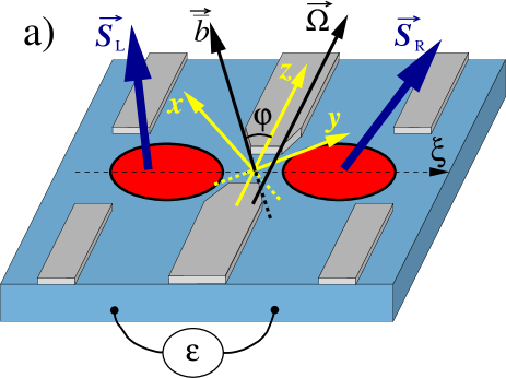
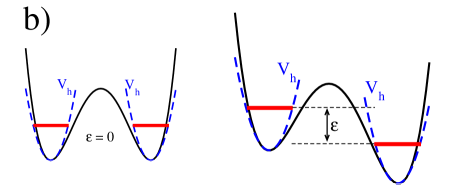
Figure 1: a) double quantum dot model and the coordinate system. ${\bf S}_{L}$ and ${\bf S}_{R}$ denote the spin-$1/2$ of the electron in the right and in the left quantum dot, respectively. The dots lie in the $\xi z$-plane and are tunnel-coupled along the $\xi$-direction (perpendicular to the $z$-axis). They can be detuned by the externally applied voltage $\varepsilon/e$. The spin orbit field $\boldsymbol{\Omega}$ points along the $z$-axis, defining the first quantization axis for the triplet states $|T_{z,\pm}\rangle$ and $|T_{z0}\rangle$ (see main text). The effective magnetic sum-field $\bar{{\bf{b}}}$ defines the second quantization axis for the triplet states $|T_{\pm}\rangle$ and $|T_{0}\rangle$. We choose the mutually orthogonal axes $x,y,z$ so that $\bar{{\bf{b}}}$ lies in the $xz$-plane. b) effect of detuning on the quantum dot levels. At zero detuning $\varepsilon=0$, an electron has the same energy on the left and right quantum dot. For nonzero detuning, the energy of an electron on the left dot is $\varepsilon$ higher than the energy of an electron on the right dot.

In addition to the terms described above, there are three sources of spin-dependent interactions: Zeeman coupling to an external magnetic field, hyperfine coupling between electron spins and nuclear spins in a quantum dot, and the spin orbit interaction. For now we neglect the spin orbit interaction, and analyze it in detail in the next section.

The direct coupling of the electron spins to a uniform external magnetic field ${\bf{B}}$ is described by the Zeeman term

$$H_{\rm Z}=-g\mu_{e}{\bf{B}}\cdot\left({\bf{S}}_{\rm L}+{\bf{S}}_{\rm R}\right),$$ (18)

where $g$ is the electron $g-$factor and $\mu_{e}$ is the electron magnetic moment. In addition, the Fermi contact hyperfine interaction between electron and nuclear spins reads

$$H_{\rm nuc}=\sum_{i}{\bf{h}}_{i}\cdot{\bf{S}}_{i},$$ (19)

where ${\bf{h}}_{i}$, $i=L,R$, is the Overhauser field of the quantum dot $i$, given by Overhauser (1953)

$${\bf{h}}_{i}=\sum_{j}A_{j}|\Psi_{i}({\bf{R}}_{j})|^{2}{\bf{I}}_{j}.$$ (20)

Here $A_{j}$ is the hyperfine coupling constant for the nuclear species at site $j$, with typical size of the order of $90\mu\rm{eV}$ for GaAs Schliemann et al. (2003), $\Psi_{i}$ is the electron orbital envelope wave function in the right ($i=R$) and left ($i=L$) dot, ${\bf{R}}_{j}$ is the position of the $j$th nucleus in the quantum dot, and ${\bf{I}}_{j}$ is the corresponding nuclear spin.

Because the Zeeman and hyperfine interactions, Eqs. (18) and (19), have similar forms, we combine them into a single effective field that acts on the electron spin in each dot:

$$H_{\rm nuc}+H_{\rm Z}=-{\bf{b}}_{\rm L}\cdot{\bf{S}}_{\rm L}-{\bf{b}}_{\rm R}\cdot{\bf{S}}_{\rm R}.$$ (21)

The effective fields ${\bf{b}}_{\rm L,R}=g\mu_{\rm B}{\bf{B}}_{\rm L,R}-{\bf{h}}_{\rm L,R}$ include the contributions of the external and Overhauser fields, with all coupling constants absorbed in the field definitions. The energy levels arising from the spin-conserving Hamiltonian, Eq. (16), along with coupling to a uniform effective field, Eq. (21) with ${\bf{b}}_{\rm L}={\bf{b}}_{R}$, are shown in the left panel of Fig. 2.

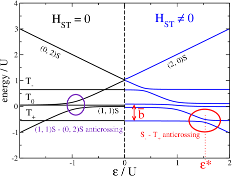
Figure 2: Energy levels of the double quantum dot system obtained from exact numerical diagonalization of $H$ given in Eq. (30) and plotted as a function of the detuning $\varepsilon$ measured in units of the Coulomb on-site repulsion energy $U$. Of particular interest here are the crossings and anti-crossings of singlet and triplet states due to spin orbit and hyperfine interactions. For $H_{\rm ST}=0$ (see Eq. (42)), i.e. vanishing singlet-triplet mixing (left-hand side of plot), the parameter values chosen are $(U,t,p,X,V_{-},V_{+},\bar{b},\delta b_{y},\delta{\bf{b}}\cdot{\bf{e}},\delta{\bf{b}}\cdot{\bf{e^{\prime}}},\varphi)=(1,0.1,0,0,0.05,0.04,0.3,0,0,0,0)$. In this case, the singlets $|(1,1)S\rangle$ and $|(0,2)S\rangle$ anti-cross (left oval) and a finite gap opens, whereas the singlets and triplets only cross (no gap). For $H_{\rm ST}\neq 0$ additional gaps open (right-hand side of plot), in particular at the lower singlet-triplet anti-crossing around $\varepsilon=\varepsilon^{*}$ (right oval) with an energy splitting $\Delta_{ST}$ that depends on magnetic field, detuning, spin orbit and hyperfine interactions (see main text and figures below). The singlet $S_{-}$ is a superposition of $|(1,1)S\rangle$ and $|(0,2)S\rangle$ (see Eq. (37)). The parameter values chosen for the right plot are $(U,t,p,X,V_{-},V_{+},\bar{b},\delta b_{y},{\delta{{\bf{b}}}\cdot{\bf{e}}},\delta{\bf{b}}\cdot{{\bf{e^{\prime}}}},\varphi)=(1,0.1,0.01,0,0.05,0.04,0.3,0.02,0.02,0.01,\pi/2)$.

Below we will be interested in transitions that change the total spin of the pair of electrons in the DQD. To facilitate the discussion, we separate the total field into a sum-field $\bar{{\bf{b}}}=({\bf{b}}_{\rm L}+{\bf{b}}_{\rm R})/2$ and a difference field $\delta{\bf{b}}=({\bf{b}}_{\rm L}-{\bf{b}}_{\rm R})/2$:

$$H_{\rm nuc}+H_{\rm Z}=-{\bf{\bar{b}}}\cdot\left({\bf{S}}_{\rm L}+{\bf{S}}_{\rm R}\right)-\delta{\bf{b}}\cdot\left({\bf{S}}_{\rm L}-{\bf{S}}_{\rm R}\right).$$ (22)

The symmetric component $\bar{{\bf{b}}}$ conserves the magnitude of the total spin, $\left[\bar{{\bf{b}}},\left({\bf{S}}_{\rm L}+{\bf{S}}_{\rm R}\right)^{2}\right]=0$, while the antisymmetric component $\delta{\bf{b}}$ does not. We include the spin-conserving field $\bar{{\bf{b}}}$ into the unperturbed Hamiltonian, and define

$$H_{\rm TT}=H_{TT,0}-\bar{{\bf{b}}}\cdot\left({\bf{S}}_{\rm L}+{\bf{S}}_{\rm R}\right).$$ (23)

Below we will investigate the role of the Overhauser fields in causing spin transitions near a singlet-triplet level crossing in a two-electron DQD. While the external magnetic field ${\bf{B}}$ is a classical variable, the Overhauser fields ${\bf{h}}_{\rm L,R}$ are, in principle, quantum operators that involve a large number of nuclear spins, see Eq. (20). Hyperfine-induced electron spin transitions may be accompanied by nuclear spin flips, and the dynamical, quantum nature of the Overhauser field may be important. However, due to the large number of nuclear spins, the time scale for the Overhauser fields ${\bf{h}}_{\rm L,R}$ to change appreciably can be much longer than the time spent near the avoided crossing, where spin transitions are possible. Thus we will treat the fields $\bar{{\bf{b}}}$ and $\delta{\bf{b}}$ as quasi-static classical variables, including a discussion of the averaging which occurs due to nuclear Larmor precession and statistical (thermal) fluctuations.

III Spin orbit interaction

In addition to the external and hyperfine fields, electron spins in a DQD are also influenced by orbital motion due to the spin-orbit interaction. Here we describe how the bulk spin-orbit coupling of the 2DEG is manifested in the confined DQD system. In GaAs quantum wells, the spin-orbit interaction is caused by the inversion asymmetry of the interface that forms the quantum well Rashba (1960); Bychkov and Rashba (1984); Dyakonov and Kachorovskii (1986) and the inversion asymmetry of host material Dresselhaus (1955). With the 2DEG being much thinner than the lateral quantum dot dimensions, both spin orbit interactions are linear in the in-plane momenta of the confined electrons, and together are given by

$$H_{\rm SO}=\alpha\left(p_{x^{\prime}}\sigma_{y^{\prime}}-p_{y^{\prime}}\sigma_{x^{\prime}}\right)+\beta\left(-p_{x^{\prime}}\sigma_{x^{\prime}}+p_{y^{\prime}}\sigma_{y^{\prime}}\right),$$ (24)

where the Rashba and Dresselhaus spin orbit interaction constants $\alpha$ and $\beta$, respectively, depend on the thickness and shape of the confinement in the growth direction and on the material properties of the heterostructure in which the 2DEG is fabricated. This form of spin-orbit coupling appears in a quantum well fabricated in the $(001)$ plane of GaAs crystal, and the $x^{\prime}$- and $y^{\prime}$-axes point along the crystallographic directions $[100]$ and $[010]$, respectively.

Within the space of low-energy single-electron orbitals in the DQD, the action of the spin orbit interaction can be expressed in terms of a spin-orbit field $\boldsymbol{\Omega}$,

$$H_{\rm SO}=\frac{i}{2}\boldsymbol{\Omega}\cdot\sum_{\alpha,\beta=\uparrow\downarrow}\left(c^{\dagger}_{{\rm{L}}\alpha}\boldsymbol{\sigma}^{\alpha\beta}c^{\phantom{\dagger}}_{{\rm{R}}\beta}-{\rm h.c.}\right),$$ (25)

where the field

$$i{\bf{\Omega}}=\langle\Phi_{\rm L}|p_{\xi}|\Phi_{\rm R}\rangle{\boldsymbol{a}_{{\bf{\Omega}}}}$$ (26)

depends on the orientation of the dots with respect to crystallographic axes through the vector $\boldsymbol{a}_{{\bf{\Omega}}}$ Stepanenko et al. (2003). For a 2DEG in the $(001)$ plane, $\boldsymbol{a}_{{\bf{\Omega}}}$ is given by

$${\bf{a}}_{{\bf{\Omega}}}=\left(\beta-\alpha\right)\cos\theta{\bf{e}}_{[\bar{1}10]}+\left(\beta+\alpha\right)\sin\theta{\bf{e}}_{[110]},$$ (27)

where the angle between the ${\bf{e}}_{\xi}$ direction and the $[110]$ crystallographic axis is denoted by $\theta$. The matrix element of $p_{\xi}$, the momentum component along the $\xi$-direction that connects the two dots, see Fig. 1, is taken between the corresponding Wannier orbitals, and it depends on the envelope wave function and the double dot binding potential. The spin orbit field ${\bf{\Omega}}$ accounts for the spin rotation when the electron hops between the dots. Therefore, the spin orbit interaction enables transitions between triplet states with single occupation of each well, to the singlet states with double occupation of either the left or the right well.

The matrix element in Eq. (26) can be calculated explicitly in a model potential Stepanenko et al. (2003); Burkard et al. (1999), giving

$${\bf{\Omega}}=\frac{4t}{3}\frac{l}{\Lambda_{\rm SO}}\frac{\boldsymbol{a}_{{\bf{\Omega}}}}{|\boldsymbol{a}_{{\bf{\Omega}}}|},$$ (28)

where $l$ is the interdot distance. The numerical prefactor is model-dependent, but the dependence on other parameters is generic. The hopping amplitude $t$, and the interdot separation $l$ depend on the geometry of the double dot system, whereas the spin-orbit length $\Lambda_{\rm SO}$ is determined by material properties (Rashba and Dresselhaus spin orbit strength) and by the orientation of the DQD with respect to the crystallographic axes. In particular, if the 2DEG lies in the $(001)$ plane, it is given by

$$\frac{1}{\Lambda_{\rm SO}}=\sqrt{\left(\frac{\cos\theta}{\lambda_{-}}\right)^{2}+\left(\frac{\sin\theta}{\lambda_{+}}\right)^{2}},$$ (29)

where $\lambda_{\pm}=\hbar/[m^{*}(\beta\pm\alpha)]$ Golovach et al. (2008), with $m^{*}$ being the effective band mass of the electron. In the special case $\beta=0$, $\theta=0$, this definition reduces to the Rashba spin orbit length $\Lambda_{\rm SO}\left|{}_{\beta=\theta=0}\right.=\lambda_{\rm SO}=\hbar/m^{*}\alpha$.

One of the main goals in the following is to derive the dependence of the energy splitting at the anticrossing between the lowest-energy electron spin triplet and singlet states (see Fig. 2, $S_{-}-T_{+}$ anticrossing) in terms of this spin-orbit length $\Lambda_{\rm SO}$. Detailed understanding of this dependence may then be used to extract the value of $\Lambda_{\rm SO}$, e.g. from measurements of the singlet-triplet transition probability in gate-sweep experiments.

Within the model used above for explicit calculation, the components of $\boldsymbol{\Omega}$ are real, even in the presence of magnetic fields. This is due to the high symmetry of the ground state orbitals of the quantum dot in the model, and remains true even after the replacement $p_{\xi}\rightarrow p_{\xi}-(e/c)A_{\xi}$ in the spin-orbit Hamiltonian $H_{\rm SO}$, Eq. (24). However, this fact is not essential for the physics described below.

IV Singlet-triplet transitions and the choice of spin quantization axis

Transitions between singlet and triplet states can be mediated by the spin orbit interaction or by an inhomogeneous effective magnetic field (external plus hyperfine), $\delta{\bf{b}}$. In Rudner et al. (2010) it was shown that the transfer of angular momentum between electrons and the nuclei strongly depends on the relative size and phase of the electron spin flip matrix elements induced by spin orbit interaction and by the difference of the Overhauser fields in the two dots. Using our model of a detuned DQD, we will study these matrix elements in the following in detail and in particular focus on the singlet-triplet level splitting, see Fig. 2, right panel.

The homogeneous field $\bar{{\bf{b}}}$ acts only within the spin triplet subspace, while the inhomogeneous field $\delta{\bf{b}}$ mixes singlet $S=0$ and triplet $S=1$ states. Representing the total Hamiltonian in the basis $\{(|(0,2)S\rangle,|(2,0)S\rangle,|(1,1)S\rangle,|T_{z+}\rangle,|T_{z0}\rangle,|T_{z-}\rangle)\}$, where the $z$-axis is taken along $\boldsymbol{\Omega}$, see Fig. 1, we find

$$H=\left(\begin{array}[]{cccccc}U-\varepsilon&X&-\sqrt{2}t&0&-i\sqrt{2}\Omega&0\\ X&U+\varepsilon&-\sqrt{2}t&0&-i\sqrt{2}\Omega&0\\ -\sqrt{2}t&-\sqrt{2}t&V_{+}&-\sqrt{2}\left(\delta b_{x}-i\delta b_{y}\right)&2\delta b_{z}&\sqrt{2}\left(\delta b_{x}+i\delta b_{y}\right)\\ 0&0&-\sqrt{2}\left(\delta b_{x}+i\delta b_{y}\right)&V_{-}+2\bar{b}_{z}&\bar{b}_{x}\sqrt{2}&0\\ i\sqrt{2}\Omega&i\sqrt{2}\Omega&2\delta b_{z}&\bar{b}_{x}\sqrt{2}&V_{-}&\bar{b}_{x}\sqrt{2}\\ 0&0&\sqrt{2}\left(\delta b_{x}-i\delta b_{y}\right)&0&\bar{b}_{x}\sqrt{2}&V_{-}-2\bar{b}_{z}\end{array}\right).$$ (30)

The Hamiltonian $H$, Eq. (30), is the starting point for all of our further calculations. Our results will show the dependence of the singlet-triplet splitting on the parameters that enter $H$. This Hamiltonian describes a double quantum dot with single orbital per dot, i.e. in the Hund-Mulliken approximation, and it is valid as long as the dot quantization energy is the largest energy scale in the problem. It can be applied to double quantum dots of various kinds, for example the gated lateral or vertical dots in III-V semiconductor materials, quantum dots in nanowires, or self assembled quantum dots. We illustrate the spectrum of $H$ in Fig. 2, for a set of parameters that emphasizes anticrossings of the levels. The spectrum is obtained by exact diagonalization of $H$, and it is given as a function of detuning $\epsilon$. For other types of quantum dots, the parameter values would change, but the overall structure of the spectrum remains the same.

V Effective Hamiltonian near the singlet-triplet anticrossing

In the limit of large detuning, $|\varepsilon|\gg U,V_{+},V_{-},|\bar{{\bf{b}}}|$, the ground state is a spin singlet with both electrons in either the left or right dot, depending on whether $\varepsilon>0$ or $\varepsilon<0$. In the region of weak detuning, the ground state has one electron in each of the dots. For a sufficiently strong sum-field, $|\bar{{\bf{b}}}|>U-V_{+}$, the singlet ground state exhibits an avoided level crossing with the lowest energy triplet state, i.e. the $S=1$ state oriented along $\bar{{\bf{b}}}$, see Fig. 1, at a detuning where the potential energy gained by the singlet’s double occupancy of the lower well compensates the Zeeman energy gained by the spin-polarized triplet. Here, the residual splitting is determined by the spin non-conserving interactions. The behavior near this anticrossing has been the focus of many recent studies on the interaction of electron spins with the nuclei Reilly et al. (2008a, b); Barthel et al. (2009); Bluhm et al. (2010); Schroer et al. (2011). The role of spin orbit interaction has received less attention than that of the nuclei, and will be analyzed in the following sections.

The orbital structure of the levels near the anticrossing is determined by the spin-independent interactions and by the direction and amplitude of the sum-field $\bar{{\bf{b}}}$. The singlet subspace acted on by the Hamiltonian in Eq. (17) includes a state with single occupation of the two dots, and two states which feature double occupation of either the left or the right dot. Generically, the state that takes part in the anticrossing includes amplitudes of all three singlet states. However, because $U\gg J$, where $J\approx 4t^{2}/(U-V_{+})\sim 0.01-0.1\,{\rm meV}$ is the splitting between the lowest-energy triplet and the lowest-energy singlet state, and $U\sim 1\,{\rm meV}$, admixture of at least one of the singlets will always be suppressed at the anticrossing by a large energy denominator (note that $t\approx 0.01-0.1\,{\rm meV}\ll U-V_{+})$.

Let us now construct the effective Hamiltonian which acts in the two-level subspace spanned by the levels near the anticrossing. First, the spin-conserving part of the full (6$\times$6) Hamiltonian reads

$$H_{\rm sc}=\left(\begin{array}[]{cc}H_{\rm SS}&0\\ 0&H_{\rm TT}\end{array}\right),$$ (31)

where the block $H_{\rm SS}$ acts in the singlet subspace, $H_{\rm TT}$ acts in the triplet subspace, and the off-diagonal blocks vanish due to spin conservation.

Explicitly, the block $H_{\rm SS}$ is given by Eq. (17) in the basis Eq. (3)-(8). The triplet block $H_{\rm TT}$ is given in Eq. (23). Since $U\gg t\gg X$ in a typical quantum dot, the state at the anticrossing can at most include significant contributions from two out of three basis singlets. We will consider the anticrossing at positive values of the detuning $\varepsilon$ (the anticrossing at negative voltage is analogous) so that the $|(2,0)S\rangle$ state with the energy $U+\varepsilon$ is far detuned from the other two singlets. The remaining two singlets can be close in energy. In order to include the possibility of near degeneracy, we will introduce a mixing angle $\psi$ that parametrizes the hybridization of the $|(0,2)S\rangle$ and $|(1,1)S\rangle$ states. In the restricted subspace of these hybridized states, the singlet Hamiltonian reads:

$$H_{\rm r}=\frac{U-\varepsilon+V_{+}}{2}+\boldsymbol{\tau}\cdot{\bf{n}}\sqrt{\frac{(U-\varepsilon-V_{+})^{2}}{4}+2t^{2}},$$ (32)

where $\boldsymbol{\tau}=(\tau_{x},\tau_{y},\tau_{z})$ is the vector of Pauli matrices. The pseudospin $\boldsymbol{\tau}$ describes the components of the anticrossing singlet state, $|\tau_{z}=1\rangle=|(1,1)S\rangle$, $|\tau_{z}=-1\rangle=|(0,2)S\rangle$, within the approximation that we neglect the remaining $|(2,0)S\rangle$ component (this is valid when $|t/U|\ll 1$). In this case, ${\bf{n}}={\bf{e}}_{z}\cos{2\psi}+{\bf{e}}_{x}\sin{2\psi}$ is a unit vector parametrized by the mixing angle $\psi$ that describes the relative size of mixing and splitting of $\tau_{z}$ eigenstates. Note that the $y$-component of ${\bf{n}}$ vanishes due to the choice of phases in the quantum dot ground states, which guarantees that the spin-independent hopping matrix element $t$ is purely real. We remark again that in our DQD set-up the hopping matrix element $t$ stays real even in the presence of magnetic fields, Burkard et al. (1999). The mixing angle of the doubly and singly occupied states at the $S=0$ anticrossing, $|(0,2)S\rangle$ and $|(1,1)S\rangle$, respectively, is defined by

$$\cos{2\psi} =\frac{U-V_{+}-\varepsilon}{\sqrt{\left(U-V_{+}-\varepsilon\right)^{2}+8t^{2}}},$$ (33)

$$\sin{2\psi} =\frac{2\sqrt{2}t}{\sqrt{\left(U-V_{+}-\varepsilon\right)^{2}+8t^{2}}}.$$ (34)

In the basis of eigenstates of Eq. (32) the singlet Hamiltonian $H_{\rm SS}$ is given by

$$H_{\rm SS}=\left(\begin{array}[]{ccc}U+\varepsilon&X\cos\psi-\sqrt{2}t\sin\psi&-X\sin\psi-\sqrt{2}t\cos\psi\\ X\cos\psi-\sqrt{2}t\sin\psi&E_{S+}&0\\ -X\sin\psi-\sqrt{2}t\cos\psi&0&E_{S-}\end{array}\right),$$ (35)

where

$$E_{S\pm}=\frac{U-\varepsilon+V_{+}}{2}\pm\sqrt{(U-\varepsilon-V_{+})^{2}/4+2t^{2}}$$ (36)

are the eigenvalues of $H_{\rm SS}$ in the spin-conserving sector. The basis vectors used here are the far-detuned singlet $|(2,0)S\rangle$ (Eq. (3)) and the singlets $|S_{\pm}\rangle$ defined by

$$|S_{+}\rangle =\sin\psi|(1,1)S\rangle-\cos\psi|(0,2)S\rangle,$$ (37)

$$|S_{-}\rangle =\cos\psi|(1,1)S\rangle+\sin\psi|(0,2)S\rangle.$$ (38)

In the limit $U\gg t$, $|S_{\pm}\rangle$ become eigenstates of $H_{\rm SS}$ with energies $E_{\rm S\pm}$ given in Eq. (36).

While the mixing of orbital states belonging to singlets does not affect the triplet Hamiltonian $H_{\rm TT}$, it will change the form of coupling between the singlet and triplet states near the anticrossing. In the following, we first diagonalize the triplet sector in order to find the explicit form of the triplet state at the anticrossing, and then find the effective Hamiltonian of the singlet-triplet coupling.

The triplets are Zeeman split by the sum-field $\bar{{\bf{b}}}$. We have chosen the $z$-axis of spin quantization so that the spin-orbit interaction couples $|(0,2)S\rangle$ and $|(2,0)S\rangle$ to the $|S=1,S_{z}=1\rangle$ state. We will now diagonalize the triplet part of the spin-conserving Hamiltonian, given by

$$H_{\rm TT}=V_{-}+2\bar{b}\left(\begin{array}[]{ccc}-\cos\varphi&\frac{1}{\sqrt{2}}\sin\varphi&0\\ \frac{1}{\sqrt{2}}\sin\varphi&0&\frac{1}{\sqrt{2}}\sin\varphi\\ 0&\frac{1}{\sqrt{2}}\sin\varphi&\cos\varphi\end{array}\right),$$ (39)

where we have used $\bar{b}=|\bar{{\bf{b}}}|$, $\cos\varphi=\bar{b}_{z}/\bar{b}$, and $\sin\varphi=\bar{b}_{x}/\bar{b}$ (see Fig. 1). The unitary transformation $U^{\phantom{\dagger}}_{\rm t}H_{\rm TT}U^{\dagger}_{\rm t}$ that diagonalizes $H_{\rm TT}$ is

$$U_{\rm t}=\left(\begin{array}[]{ccc}\cos^{2}\frac{\varphi}{2}&-\frac{1}{\sqrt{2}}\sin\varphi&\sin^{2}\frac{\varphi}{2}\\ -\frac{1}{\sqrt{2}}\sin\varphi&-\cos\varphi&\frac{1}{\sqrt{2}}\sin\varphi\\ \sin^{2}\frac{\varphi}{2}&\frac{1}{\sqrt{2}}\sin\varphi&\cos^{2}\frac{\varphi}{2}\end{array}\right).$$ (40)

We denote the basis states by $|T_{+}\rangle$, $|T_{0}\rangle$, and $|T_{-}\rangle$, where, now, the quantization axis is given by the sum-field $\bar{{\bf{b}}}$.

With the diagonalization of the triplet block of the spin-conserving Hamiltonian, and the preceding approximate diagonalization of the spin-conserving singlet Hamiltonian, Eq. (35), we are able to describe the spin-conserving interaction near the anticrossing in a convenient form. We will use $|S_{-}\rangle$ and $|T_{+}\rangle$ as basis vectors, and study the effective Hamiltonian in the vicinity of the anticrossing that can emerge from spin non-conserving interactions.

The full Hamiltonian is

$$H=H_{\rm sc}+H_{\rm SO}-\delta{{\bf{b}}}\cdot\left({\bf{S}}_{\rm L}-{\bf{S}}_{\rm R}\right),$$ (41)

and reads in block form

$$H=\left(\begin{array}[]{cc}H_{\rm SS}&H_{\rm ST}\\ H_{\rm TS}&H_{\rm TT}\end{array}\right).$$ (42)

The diagonal blocks $H_{\rm SS}$ and $H_{\rm TT}$ give the spin-conserving part, denoted by $H_{\rm sc}$, while the off-diagonal blocks $H_{\rm ST}$ and $H_{\rm TS}=H_{\rm ST}^{\dagger}$ induce singlet-triplet transitions. In the basis $(|(2,0)S\rangle,|S_{+}\rangle,|S_{-}\rangle,|T_{+}\rangle,|T_{0}\rangle,|T_{-}\rangle)$, the diagonal blocks take a simple form. The singlet block is $H_{\rm SS}$ given in Eq. (35). The triplet block $H_{\rm TT}$ is diagonal and reads

$$H_{\rm TT}={\rm diag}\left(V_{-}-|\bar{{\bf{b}}}|,V_{-},V_{-}+|\bar{{\bf{b}}}|\right),$$ (43)

where we used that $|T_{+}\rangle$ is the lowest-energy triplet.

The effective Hamiltonian near the anticrossing is determined by the spin-conserving terms $t,U,X,\varepsilon,\bar{{\bf{b}}}$, and by the spin non-conserving terms $\boldsymbol{\Omega}$, arising from spin-orbit coupling, and $\delta{\bf{b}}$, the effective difference field. All these interactions can be treated perturbatively in dots with weak overlap of the orbitals. The off-diagonal terms are denoted by $H_{\rm ST}=H_{\rm ST}^{\rm SO}+H_{\rm ST}^{\rm\delta b}$, and $H_{\rm TS}=H_{\rm ST}^{\dagger}$, where

$$H_{\rm ST}^{\rm SO}=i\Omega\left(\begin{array}[]{ccc}-\sin{\varphi}&-\sqrt{2}\cos{\varphi}&\sin{\varphi}\\ \cos{\psi}\sin{\varphi}&\sqrt{2}\cos{\psi}\cos{\varphi}&-\cos{\psi}\sin{\varphi}\\ -\sin{\psi}\sin{\varphi}&-\sqrt{2}\sin{\psi}\cos{\varphi}&\sin{\psi}\sin{\varphi}\end{array}\right),$$ (44)

$$H_{\rm ST}^{\rm\delta{{\bf{b}}}}=\left(\begin{array}[]{ccc}0&0&0\\ \sqrt{2}\left(i\delta b_{y}+\delta{\bf{b}}\cdot{\bf{e^{\prime}}}\right)\sin\psi&2\left(\delta{\bf{b}}\cdot{\bf{e}}\right)\sin\psi&\sqrt{2}\left(i\delta b_{y}-\delta{\bf{b}}\cdot{\bf{e^{\prime}}}\right)\sin\psi\\ \sqrt{2}\left(i\delta b_{y}+\delta{\bf{b}}\cdot{\bf{e^{\prime}}}\right)\cos\psi&2\left(\delta{\bf{b}}\cdot{\bf{e}}\right)\cos\psi&\sqrt{2}\left(i\delta b_{y}-\delta{\bf{b}}\cdot{\bf{e^{\prime}}}\right)\cos\psi\end{array}\right),$$ (45)

where the unit vector

$${\bf{e}}={\bf{e}}_{x}\sin\varphi+{\bf{e}}_{z}\cos\varphi$$ (46)

points in the direction of the homogeneous field $\bar{{\bf{b}}}$, and the vector

$${\bf{e^{\prime}}}=-{\bf{e}}_{x}\cos\varphi+{\bf{e}}_{z}\sin\varphi$$ (47)

lies in the $xz$-plane, which contains ${\boldsymbol{\Omega}}$ and $\bar{{\bf{b}}}$, and points in the direction normal to $\bar{{\bf{b}}}$.

In the vicinity of the anticrossing, the DQD behaves as an effective two-level system, with the dynamics described by an effective Hamiltonian denoted by $H_{\rm cr}$. Up to first order in spin non-conserving interactions and, after neglecting the high-energy state $|(2,0)S\rangle$, we find

$$H_{\rm cr}^{(1)}=\left(\begin{array}[]{cc}E_{S-}&H_{34}\\ H_{43}&E_{T+}\end{array}\right),$$ (48)

where $H_{34}=\langle S_{-}|H|T_{+}\rangle$ is the matrix element of $H$, Eq. (42), between the anticrossing states, and $E_{T+}=V_{-}-\bar{b}$.

VI Singlet-triplet splitting at the anticrossing

The singlet-triplet splitting $\Delta_{\rm ST}$ at the $S_{-}-T_{+}$ anticrossing, see Fig. 2, can be accessed in the spin blockade regime by transport measurements or by charge sensing. This splitting gives valuable information about the properties of the quantum dots and the nuclear polarization. We shall derive now explicit expressions for $\Delta_{\rm ST}$ in terms of the experimentally relevant quantities $\varepsilon$, $\bar{{\bf{b}}}$, $\delta{\bf{b}}$, and ${\bf{\Omega}}$. We proceed by perturbation expansion in $H_{\rm ST}$, $t/U$, and $X/U$. First, we focus on the first-order contributions and afterward address the higher order corrections which become relevant around the points where the leading contributions can be tuned to zero by the control parameters.

As the DQD detuning $\varepsilon$ is varied with other parameters held fixed, there is a special value $\varepsilon^{*}$ where the energy $E_{S-}$ of the lowest singlet, Eq. (36), becomes equal to the energy $E_{T+}=V_{-}-\bar{b}$ of the triplet $|T+\rangle$, Eq. (43). The detuning at which this crossing occurs is controlled by the amplitude $\bar{b}$ of the sum-field, as well as the tunnel coupling $t$. For the unperturbed case, described by $H_{0}$, $\varepsilon^{*}$ is the solution of the equation

$$E_{\rm S-}(\varepsilon^{*})=V_{-}-\bar{b}.$$ (49)

When the spin non-conserving interactions are taken into account, the crossing of singlet ($S=0$) and triplet ($S=1$) states is avoided due to state mixing (hybridization).

Up to first order in $H_{\rm ST}$, $t/U$, and $X/U$, the splitting follows from Eq. (48) and reads

$$\Delta_{\rm ST}(\varepsilon,\bar{b},\varphi)=2\sqrt{|H_{34}|^{2}+(E_{S-}-E_{T_{+}})^{2}}.$$ (50)

For a fixed value of $\bar{b}$, the splitting attains its minimum value $\Delta^{*}_{\rm ST}$ at $\varepsilon^{*}$,

$$\Delta^{*}_{\rm ST}\equiv\Delta_{\rm ST}(\varepsilon^{*}(\bar{b}),\bar{b},\varphi)=\min_{\varepsilon}\Delta_{\rm ST}(\varepsilon,\bar{b},\varphi),$$ (51)

where $\varepsilon^{*}$ implicitly depends on $\bar{b}$, as well as other DQD parameters. From Eqs. (48), (44), and (45), the splitting is equal to $2|H_{34}|$,

$$\Delta^{*}_{\rm ST}=2\left|-i\Omega\sin\varphi\sin\psi+\sqrt{2}\left(\delta{\bf{b}}\cdot{\bf{e^{\prime}}}+i\delta b_{y}\right)\cos\psi\right|.$$ (52)

Note that $\Delta^{*}_{\rm ST}$ contains contributions from both the spin-orbit coupling and the difference field $\delta{\bf{b}}$. The relative importance of each of the two terms depends on the detuning $\varepsilon^{*}$ through the mixing angle $\psi$, as well as on the geometry through the angle $\varphi$ between the effective field $\bar{{\bf{b}}}$ and the spin-orbit field ${\bf{\Omega}}$. When varying the detuning $\varepsilon$ from large to small values, $\psi$ decreases from $\psi\approx\pi/2$ at strong detuning, $\varepsilon\gg U-V_{+}$, to $\psi\approx 0$ at $|\varepsilon|\ll t$. For a mixing angle $\psi\approx\pi/2$, the contribution to $\Delta^{*}_{\rm ST}$ coming from the spin orbit interaction dominates the one from the difference-field, and vice versa for $\psi\approx 0$.

Reaching the $\psi\approx 0$ regime requires weak magnetic fields, i.e. $\bar{{b}}\ll t$, and in this case the energy splittings between the triplet states are not large enough to make use of the simple model for a two-level anticrossing. On the other hand, reaching the regime with $\psi\approx\pi/2$ requires that the detuning $\varepsilon^{*}$ at which $|S_{-}\rangle$ and $|T_{+}\rangle$ anticross is far away from $\varepsilon_{12}$, the detuning at the anticrossing of $|(1,1)S\rangle$ and $|(0,2)S\rangle$ singlets, cf. Fig. 2. The width of the $|(1,1)S\rangle-|(0,2)S\rangle$ anticrossing is of the order $t$, so the requirement is $|\varepsilon^{*}-\varepsilon_{12}|\gg t$. Therefore, the Zeeman energy of $|T_{+}\rangle$ must be larger than $t$, so $g\mu_{\rm B}B\gg t$, which gives $B\gg 0.2\,{\rm T}$ for typical values $t\sim 10\,{\rm\mu eV}$ and $|g|=0.4$.

These considerations show that, at least in principle, the relative strengths of the spin-orbit and hyperfine contributions to the singlet-triplet coupling can be tuned through a wide range of values using a combination of gate voltages and magnetic field strength and direction. What situation do we expect for typical GaAs dots? Using a value of 3-5 mT for the random hyperfine field (see e.g. Ref. Hanson et al. (2007) and references therein), and an electron $g$-factor $|g|=0.4$, we estimate $|\delta b|\approx 70-120$ neV. For the spin-orbit coupling $\Omega$, see Eq.(28), using $t=10\mu eV$, an interdot separation $l=50$ nm, and a spin-orbit length $\Lambda_{\rm SO}$ in the range 6-30 $\mu$m (see e.g. Refs.Zumbühl et al. (2002); Nowack et al. (2007)), we find $|\Omega|\approx 20-110$ neV. Parameters may vary from device to device, but it appears that the spin-orbit and hyperfine couplings are generally of similar orders of magnitude, with the spin-orbit coupling typically a few times weaker. Thus adjustments of the matrix elements over a reasonable range of $\psi$ may be sufficient to explore both the hyperfine and spin-orbit dominated regimes. Similar analysis can be performed for devices in other materials, such as InAs or InSb nanowires, where the natural balance between hyperfine and spin-orbit couplings may shift.

VI.1 Singlet-triplet splitting $\Delta_{\rm ST}^{*}$ for ${\bf{\delta b}}=0$

Let us first consider the special case of vanishing difference field, $\delta{\bf{b}}=0$, and finite uniform field, $\bar{{\bf{b}}}\neq 0$. In this case, the splitting depends not only on $\boldsymbol{\Omega}$ but also on the detuning at the minimal splitting, $\varepsilon^{*}$, which itself is implicitly determined by the sum-field amplitude $\bar{{b}}$. The geometry of the system enters through the angle $\varphi$ between $\bar{b}$ and the spin-orbit field $\boldsymbol{\Omega}$. In Fig. 3 we show a plot of the level splitting $\Delta_{\rm ST}(\varepsilon^{*},\bar{b},\varphi)$, given in Eq. (52) as a function of its variables and for $\delta{\bf{b}}=0$.

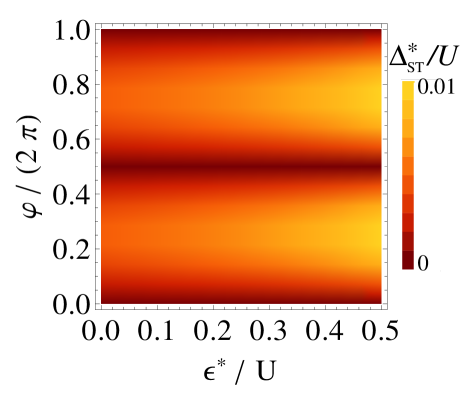
Figure 3: Singlet-triplet level splitting $\Delta^{*}_{\rm ST}=\Delta_{\rm ST}(\varepsilon^{*},\bar{b},\varphi)$, Eq. (52), for $\delta{\bf{b}}=0$ (no nuclear field), as a function of the detuning $\varepsilon^{*}$ at which the crossing occurs (cf. Fig. 2) and of the angle $\varphi$ between the spin-orbit field ${\bf{\Omega}}$ and the magnetic sum-field $\bar{\bf b}$ (cf. Fig. 1). Parameters used for this plot are $U=1$, $t=0.01$, $V_{+}=0.75$, $\delta{\bf{b}}=0$.

At any fixed angle $\varphi\neq 0$, $\Delta^{*}_{\rm ST}$ shows a dependence on the detuning $\varepsilon^{*}$ at the anticrossing due to the mixing of $|(0,2)S\rangle$, which is coupled to $|T_{+}\rangle$ via the spin-orbit interaction, and $|(1,1)S\rangle$, which does not couple to $|T_{+}\rangle$ via spin-orbit coupling in the first order, see Fig.4. At large values of detuning $\varepsilon^{*}\gg U-V_{+}$, the splitting reaches a saturation value $2\Omega\sin\varphi$. For typical GaAs quantum dots, reaching this regime requires strong magnetic fields of $B\gg t$. At lower values of the detuning $\varepsilon<U-V_{+}$, the mixing of the singlet $|(1,1)S\rangle$ becomes significant, and the spin-orbit coupling value $\Omega$ cannot be read off directly from the splitting.

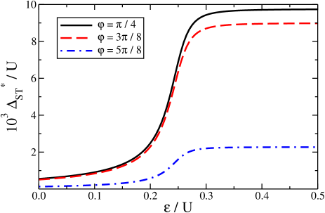
Figure 4: Singlet-triplet level splitting $\Delta^{*}_{\rm ST}=\Delta_{\rm ST}(\varepsilon^{*},\bar{b},\varphi)$, Eq. (52), for $\delta{\bf{b}}=0$ (no nuclear polarization), as a function of the detuning $\varepsilon^{*}$ at which the crossing occurs (cf. Fig. 2) and of the angle $\varphi$ between the spin-orbit field ${\bf{\Omega}}$ and the magnetic sum-field $\bar{\bf b}$ (cf. Fig. 1). At small detuning $\varepsilon^{*}<t$, the splitting becomes rather small, while it saturates at large detuning $\varepsilon^{*}>U$. The saturation value is $\propto|\sin\varphi|$, shown for $\varphi=\pi/4$ (full line), $\varphi=3\pi/8$ (dashed line) and $\varphi=5\pi/8$ (dashed-dotted line). Parameters used for this plot are $U=1$, $t=0.01$, $V_{+}=0.75$, $\delta{\bf{b}}=0$.

The maximal splitting $\Delta^{*}_{\rm ST}$ caused by spin-orbit interaction is $\Delta^{*}_{\rm ST}=2\Omega|\sin\varphi|$, for $\psi=\pi/2$. From Eq. (28) and Eq. (29), we find that $\Omega$ is set by the material properties (Dresselhaus ($\beta$) and Rashba ($\alpha$) spin orbit interactions) and the geometry of the dots. Assuming that the magnetic field is strong enough to separate the $|T_{0}\rangle$ and $|T_{-}\rangle$ states from the anticrossing, $U\gg\bar{b}\gg t\gg|{\bf{\delta b}}|$, the maximal splitting is ($|\sin\psi|=1$)

$$\Delta^{*}_{\rm ST}=\frac{4t}{3}\frac{l}{\Lambda_{\rm SO}}|\sin\varphi|,\quad({\bf{\delta b}}=0),$$ (53)

where $l$ is the interdot distance. The numeric factor (of order unity) is non-universal and depends on the specific dot geometry. Formula (53) is one of the main results of this paper. It provides a simple but useful relation between quantities that can be determined experimentally, such as $\Delta^{*}_{\rm ST}$, $t$, $l$, and $\varphi$, and a quantity of interest - the spin orbit length ${\Lambda_{\rm SO}}$. This relation could allow the strength of spin-orbit coupling to be measured experimentallyNadj-Perge et al. (2010b); Schroer et al. (2011), though the geometry and detuning-dependence must be carefully taken into account in order to obtain an accurate estimate.

Let us remark here briefly on the special case of zero detuning, i.e. $\varepsilon=0$, and weak magnetic fields. In this case, the splitting is not described by our calculations which require sufficiently large separation of the triplets in energy. However, in a slightly different system – a single quantum dot containing two electrons – singlet-triplet coupling which is forbidden by time-reversal symmetry can be generated by applying a magnetic field, $\Delta_{\rm ST}^{*}\approx(a_{\rm B}/\lambda_{\rm SO})E_{\rm Z}$ Golovach et al. (2008). This case cannot be recovered from our DQD model with one orbital per site. Indeed, here we have seen that in weak fields, ${\bar{b}}\ll t$, the coupling of the two states with single occupation in each well $|(1,1)S\rangle$ and $|T_{+}\rangle$ due to the spin-orbit interaction involves doubly occupied states which are higher in energy due to the on-site repulsion. On the other hand, for a pair of electrons in a single quantum dot, the on-site repulsion is approximately the same for both states, singlet and triplet. We note that for DQDs in weak fields, the Zeeman energy $E_{\rm Z}$, occurring in the splitting for a single dot Golovach et al. (2008), gets replaced by the exchange energy $J$ if the mixing of triplets due to $\delta{\bf{b}}\neq 0$ is neglected.

VI.2 Singlet-triplet splitting $\Delta_{\rm ST}^{*}$ for ${\bf{\delta b}}\neq 0$

In addition to spin-orbit coupling of the anticrossing triplet to $|(0,2)S\rangle$, the anticrossing triplet is coupled to the singlet $|(1,1)S\rangle$ through the difference-field $\delta{\bf{b}}$. The previous considerations show that the contributions from the difference-field $\delta{\bf{b}}$ to the splitting cannot be neglected for angles $\varphi\sim 0,\pi$, or for field strengths where $\varepsilon^{*}<U-V_{+}$, which is often be the case. Therefore, we now discuss the splitting in the presence of both, the spin-orbit field $\boldsymbol{\Omega}$ and $\delta{\bf{b}}$. The splitting $\Delta^{*}_{\rm ST}$ as a function of detuning $\varepsilon^{*}$ and direction of $\bar{{\bf{b}}}$ is shown in Fig. 5.

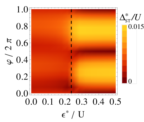
Figure 5: The same plot of the singlet-triplet splitting as in Fig. 3 except for finite nuclear polarization chosen to be $\delta{\bf{b}}=(-0.0006,0.0008,0.0012)$. In the strong detuning regime, $\varepsilon^{*}>U-V_{+}$ on the right-hand side of the plot, the splitting is determined by spin orbit interaction, $v_{\rm SO}>v_{\rm HF}$ and resembles the same area in Fig. 3. In the weak detuning regime, $\varepsilon^{*}<U-V_{+}$ on the left-hand side of the plot, the hyperfine interaction increases the splitting. The regime with similar strengths of the interactions, $v_{\rm SO}\sim v_{\rm HF}$ can be identified in the region $\varepsilon^{*}\approx U-V_{+}=0.25U$. For $\varepsilon^{*}$ on the left-hand side of the vertical dashed line, and $\varphi\approx 0,\pi$, the splitting is dominated by hyperfine interaction $v_{\rm HF}>v_{\rm SO}$. Near the dotted line, and for the angles $\varphi\approx\pi/2,3\pi/2$ the sizes of spin orbit and hyperfine interactions are similar $v_{\rm SO}\approx v_{\rm HF}$.

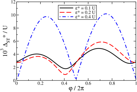
Figure 6: First order singlet-triplet splitting $\Delta^{*}_{\rm ST}=\Delta_{\rm ST}(\varepsilon^{*},\bar{b},\varphi)$, Eq. (52), for finite nuclear polarization $\delta{\bf{b}}\neq 0$, plotted as function of the angle $\varphi$ (cf. Fig. 1), for various detunings $\varepsilon^{*}$ (cf. Fig. 2). The parameters used for the plot are $U=1$, $t=0.01$, $V_{+}=0.75$, $V_{-}=0.74$, $\Omega=0.005$, and $\delta{\bf{b}}=(-0.0006,0.0008,0.0012)$. The curves correspond to $\varepsilon^{*}=0.1$ (full line), $\varepsilon^{*}=0.2$ (dashed), $\varepsilon^{*}=0.4$ (dashed-dotted). In the strong detuning regime (dashed-dotted line) the angular dependence reflects the $|\sin\varphi|$ dependence of the spin-orbit term (see Eq. (53). The regime of weaker detuning (full and dashed line) shows the hyperfine effects.

When both sources of splitting are present, generically, the gap $\Delta^{*}_{\rm ST}$ remains open. The spin-orbit contribution to Eq. (52) is always purely imaginary, while the $\delta{\bf{b}}$-contribution has both a real part, coming from the component lying in the $xz$-plane, and an imaginary part, coming from the perpendicular component $\delta b_{y}$. For any fixed value of the spin-orbit coupling strength, closing the gap would require fine tuning of $\delta{\bf{b}}$, both in amplitude and direction. As a function of the direction of $\bar{{\bf{b}}}$ the contributions to $\Delta^{*}_{\rm ST}$ compete, and, in addition, the relative size of the competing terms will change as a function of $\varepsilon^{*}$. Indeed, the spin-orbit term is strongest at large detuning $\varepsilon^{*}\gg U-V_{+}$, while the difference-field term becomes significant at small detuning $\varepsilon^{*}\sim t$. This competition affects the form of the $\varphi$-dependent splitting, see Fig.6.

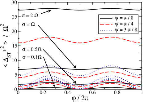
Figure 7: Square of the splitting $\langle\Delta_{\rm ST}^{*2}\rangle$, Eq. (52), averaged over Gaussian fluctuations of $\delta{\bf{b}}$ with zero mean and standard deviation $\sigma$. The plots show the dependence of $\langle\Delta_{\rm ST}^{*2}\rangle$ on the angle $\varphi$ for various mixing angles $\psi$. We have assumed isotropic Gaussian fluctuations with a standard deviation $\sigma$. Plots are for the values $\sigma/\Omega=0.1,0.5,1,2$ and illustrate the effects of various strengths of fluctuations. The curves are found by numerical averaging over the fields $\delta{\bf{b}}$.

In the limit $|{\bf{\Omega}}\sin\psi|\ll|\delta{\bf{b}}\cos\psi|$, the splitting $\Delta^{*}_{\rm ST}$ is caused mostly by the inhomogeneous field. In this case, the splitting is proportional to the size of component $\delta{\bf{b}}_{\rm\perp}=\delta{\bf{b}}-{\bf{e}}(\delta{\bf{b}}\cdot{\bf{e}})$ of $\delta{\bf{b}}$ which is normal to the homogeneous field $\bar{{\bf{b}}}=|\bar{{\bf{b}}}|{\bf{e}}$. With the leading spin-orbit coupling correction, the splitting is [see Eq.(52)]

$$\Delta^{*}_{\rm ST}=2\sqrt{2}|\delta{\bf{b}}_{\perp}\cos{\psi}|-\frac{2\Omega\delta b_{y}\sin\psi\cos\psi}{|\delta{\bf{b}}_{\perp}\cos\psi|}.$$ (54)

VI.3 Measuring the singlet-triplet coupling

The singlet-triplet coupling $\Delta_{\rm ST}^{*}$ is manifested experimentally, for example, in the spin flip probability when the system is taken through the level crossing during a time-dependent gate sweep Petta et al. (2008). In such experiments, the system is initialized to its ground state at large $\epsilon$, the $(0,2)$ singlet. When $\epsilon$ is then ramped to take the system through the singlet-triplet crossing, the two-electron spin state may change, with a probability determined by a combination of the coupling $\Delta_{\rm ST}^{*}$ and the sweep rate. The final spin state can then be read out by quickly ramping back to large $\epsilon$, where the singlet and triplet states have discernibly different charge distributions, which can be detected by a nearby charge sensor.

Even with single-shot spin detection Barthel et al. (2009), determining the spin flip probability requires building up statistics over many experimental runs. Within each run, the parameters in Eq. (52) may be considered fixed. However, the hyperfine field components are in general a priori unknown: under typical experimental conditions, the temperature is high compared with all intrinsic energy scales within the nuclear spin system, and the equilibrium state is nearly completely random. Depending on the measurement timescale, the nuclear fields on subsequent experimental runs may either remain constant or may change. While the correlation time for the longitudinal component of the nuclear field (parallel to the external field) may be quite long, the transverse components change on the timescale of nuclear Larmor precession, which for moderate fields of a few hundred millitesla can reach the sub-microsecond timescale. The coherence time associated with this precession may reach several hundred microseconds to one millisecond.

Let $P(\Delta^{*}_{\rm ST})$ be the probability that the system makes a transition to the triplet state in a single sweep, when the value of $\Delta^{*}_{\rm ST}$ is specified. In an experiment where measurements of the singlet and triplet fractions are averaged over a time long compared to all nuclear spin relaxation times, one obtains an averaged probability $\langle P(\Delta^{*}_{\rm ST})\rangle$, where $\langle A\rangle$ denotes the mean value of quantity $A$, averaging over a Gaussian distribution of $\delta{\bf{b}}$, while other parameters such as $B,t,\bar{b},\phi$ and the sweep rate are held fixed. If the measurements are averaged over a shorter period, which is long compared to the time for phase relaxation of the nuclear spins, but short compared to the longitudinal relaxation times, then the Gaussian average should be taken only over the transverse components of $\delta{\bf{b}}$, while the component parallel to the applied magnetic field is held fixed.

When the sweep rate through the S-T transition is rapid, the probability $P(\Delta^{*}_{\rm ST})$ should be proportional to $(\Delta^{*}_{\rm ST})^{2}$, so an average value of $P(\Delta^{*}_{\rm ST})$ will measure the mean value of $(\Delta^{*}_{\rm ST})^{2}$. For lower values of the sweep rate, $P$ will have corrections due to $(\Delta^{*}_{\rm ST})^{4}$, etc.. Therefore, measurements of the averaged value $\langle P(\Delta^{*}_{\rm ST})\rangle$ for a wide range of sweep rates should, in principle, yield average values of all powers of $(\Delta^{*}_{\rm ST})^{2}$, and thus allow one to deduce the probability distribution for $(\Delta^{*}_{\rm ST})^{2}$. Here we concentrate on the mean value of $(\Delta^{*}_{\rm ST})^{2}$ , and discuss predictions for this mean value as a function of the parameters $B,\phi,$ and $t$.

We illustrate the dependence of $\langle(\Delta_{\rm ST}^{*})^{2}\rangle$ on the angle $\varphi$ and mixing $\psi$ in Fig. 7 and Fig. 8. The dependence of the splitting on the angle $\varphi$, inherent in the non-averaged splitting, see Eq. (52), remains visible when the splitting is dominated by spin-orbit interaction. As expected, the dependence of the splitting on the angle $\varphi$, Fig. 7, is most visible in the case of weak fluctuations of ${\bf{\delta b}}$, i.e. for weak hyperfine coupling. In addition, the angular dependence is more pronounced for larger mixing angles, since the spin-orbit induced splitting depends on $\Omega\sin\psi$, Fig. 8.

The fluctuating difference field, besides changing the average $\langle(\Delta_{\rm ST}^{*})^{2}\rangle$, introduces noise in the splitting. We find that the standard deviation $\sigma_{\Delta}$ of the splitting, in the limit of weak fluctuations $|\Omega\sin\varphi\sin\psi|\gg\sigma$ is

$$\sigma_{\rm\Delta,G}=2\sigma|\cos\psi|,$$ (55)

so that it also shows dependence on the mixing angle $\psi$.

Fluctuations in $\delta{\bf{b}}$ smear the splitting at the anticrossing $\Delta_{\rm ST}^{*}$. The average value and noise in the splitting can be used to measure the strengths of spin-orbit coupling $\Omega$ and the hyperfine field $\delta{\bf{b}}$. The relative size of fluctuations in $\Delta_{\rm ST}^{*}$, as a function of $\varphi$, has minima at $\varphi\approx\pi/2,3\pi/2$.

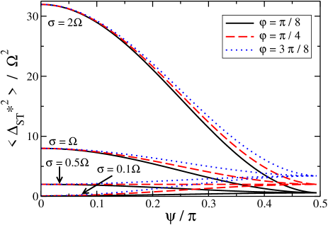
Figure 8: Average square of the splitting $\langle\Delta_{\rm ST}^{*2}\rangle$, in the fluctuating nuclear field $\delta{\bf{b}}$. The parameters are chosen as in Fig. 7, and we illustrate the dependence on the mixing angle $\psi$.

VI.4 Higher order corrections

So far, our analysis of the $|S_{-}\rangle$ - $|T_{+}\rangle$ anticrossing was based on the assumption that the largest contribution to the splitting $\Delta^{*}_{\rm ST}$, Eq. (52), results from the direct coupling of the two states via $H_{\rm ST}^{\rm SO}$ and $H_{\rm ST}^{\rm\delta{\bf{b}}}$. However, if the detuning $\varepsilon^{*}$ is not large enough to make the influence of the levels that are energetically further away from the anticrossing completely negligible, higher order terms that describe virtual transitions to such higher levels and thus involve more than one transition between the singlets and the triplets become important.

To study this regime, we derive an effective Hamiltonian in the vicinity of the anticrossing by a second order Schrieffer-Wolff (SW) transformationSchrieffer and Wolff (1966); Bravyi et al. (2011). We divide the Hilbert space of the DQD into a relevant part which includes the anticrossing states, and an auxiliary part which contains the remaining 4 states. The time-independent perturbation series is then performed in powers of the spin-non-conserving interactions. The spin-conserving Hamiltonian $H_{\rm sc}$, Eq. (31), is taken as the unperturbed part, while $H-H_{\rm sc}$ is the perturbation. In reordering the basis, we choose the crossing states $|S_{-}\rangle$ and $|T_{+}\rangle$ of $H_{\rm sc}$ to be the first two basis states. Then, the Hamiltonian has a block-diagonal form denoted by

$$H=\left(\begin{array}[]{cc}A&C\\ C^{\dagger}&B\end{array}\right),$$ (56)

where $A$ is a $2\times 2$ matrix that describes the anticrossing states, $B$ is a $4\times 4$ matrix of the states with energies far from the anticrossing and the $2\times 4$ matrix $C$ represents the coupling between of the subspaces controlled by $A$ and $B$. In the basis $\left(|S_{-}\rangle,|T_{+}\rangle,|T_{0}\rangle,|T_{-}\rangle,|(2,0)S\rangle,|S_{+}\rangle\right)$, with the two anticrossing level at the positions $1$ and $2$, we can read off the blocks from Eq. (56):

$$A=\left(\begin{array}[]{cc}E_{S-}&-i\Omega_{s}\sin\psi+\sqrt{2}\delta_{+}\cos\psi\\ i\Omega_{s}\sin\psi+\sqrt{2}\delta_{-}\cos\psi&E_{T+}\end{array}\right),$$ (57)

$$B=\left(\begin{array}[]{cccc}V_{-}&0&i\sqrt{2}\Omega_{c}&-i\sqrt{2}\Omega_{c}\cos\psi+2\delta\sin\psi\\ 0&V_{-}+\bar{b}&-i\Omega_{s}&i\Omega_{s}\cos\psi-\sqrt{2}\delta_{+}\sin\psi\\ -i\sqrt{2}\Omega_{c}&i\Omega_{s}&U+\varepsilon&-\sqrt{2}t\sin\psi-X\cos\psi\\ i\sqrt{2}\Omega_{c}\cos\psi+2\delta\sin\psi&-i\Omega_{s}\cos\psi-\sqrt{2}\delta_{-}\sin\psi&-\sqrt{2}t\sin\psi-X\cos\psi&E_{S+}\end{array}\right),$$ (58)

$$C=\left(\begin{array}[]{cccc}-i\sqrt{2}\Omega_{c}\sin\psi+2\delta\cos\psi&i\Omega_{s}\sin\psi-\sqrt{2}\delta_{-}\cos\psi&-\sqrt{2}t\cos\psi+X\sin\psi&0\\ 0&0&i\Omega_{s}&-i\Omega_{s}\cos\psi+\sqrt{2}\delta_{-}\sin\psi\end{array}\right),$$ (59)

where we have used the abbreviations $\delta=\delta{\bf{b}}\cdot{\bf{e}}$, $\delta_{\pm}=\delta{\bf{b}}\cdot{\bf{e^{\prime}}}\pm i\delta b_{y}$, $\Omega_{s}=\Omega\sin\varphi$, $\Omega_{c}=\Omega\cos\varphi$, and the unit vectors ${\bf{e^{\prime}}}$ and ${\bf{e}}$ are defined in Eq. (47) and Eq. (46), respectively.

As a result of the SW transformation on Eq. (56), the off-diagonal block $C$ is eliminated up to second order in $C$ and the transformed block $A\xrightarrow{\rm SW}A+\delta A$ becomes then the Hamiltonian of an effective two-level system. Therefore, the first-order Hamiltonian $H_{\rm cr}^{(1)}$ from Eq. (48) becomes modified by second order terms, $H_{\rm cr}\xrightarrow{\rm SW}H_{\rm cr}+\delta A$, where $\delta A$ is the second order correction to $A$. The diagonal matrix elements $\delta A_{11}$ and $\delta A_{22}$ describe the renormalization of the energy levels, and their effect is to shift the detuning $\varepsilon^{*}$ at which the anticrossing occurs. The explicit expressions of these corrections are

$$\begin{split}\delta A_{11}=&\frac{1}{E_{S-}-V_{-}}\left[2\left(\Omega_{c}\sin\psi\right)^{2}+4\delta^{2}\cos^{2}\psi\right]+\frac{1}{E_{S-}-U-\varepsilon}\left(\sqrt{2}t\cos\psi-X\sin\psi\right)^{2}+\\ &+\frac{1}{E_{S-}-V_{-}-\bar{b}}\left[2\left(\delta{\bf{b}}\cdot{\bf{e^{\prime}}}\right)^{2}\cos^{2}\psi+\left(\sqrt{2}\delta b_{y}\cos\psi+\Omega_{s}\sin\psi\right)^{2}\right],\end{split}$$ (60)

$$\delta A_{22}= \frac{1}{E_{T_{+}}-U-\varepsilon}\Omega_{s}^{2}+\frac{1}{E_{T+}-E_{S+}}\left[\left(\Omega_{s}\cos\psi+\sqrt{2}\delta b_{y}\sin\psi\right)^{2}+2\left(\delta{\bf{b}}\cdot{\bf{e^{\prime}}}\right)^{2}\sin^{2}\psi\right],$$ (61)

$$\delta A_{12}= -\frac{i}{2}\Omega_{s}\left(\sqrt{2}t\cos\psi+X\sin\psi\right)\left(\frac{1}{E_{S-}-U-\varepsilon}+\frac{1}{E_{T+}-U-\varepsilon}\right).$$ (62)

In experiments that probe the electron spin dynamics, the most important terms are the off-diagonal ones, $\delta A_{12}=\delta A_{21}^{*}$. They lead to a modification of the first order singlet-triplet splitting Eq. (51), i.e. $\Delta^{*}_{\rm ST}\xrightarrow{\rm SW}2|H_{34}+\delta A_{12}|$. Thus, up to second order, the splitting at the anticrossing becomes

$$\Delta_{\rm ST}^{*}=2\left|-i\Omega\sin\varphi\left[\sin\psi-\left(\frac{t}{\sqrt{2}}\cos\psi-\frac{X}{2}\sin\psi\right)\left(\frac{1}{E_{S-}-U-\varepsilon^{*}}+\frac{1}{E_{T+}-U-\varepsilon^{*}}\right)\right]+\sqrt{2}\left(\delta{\bf{b}}\cdot{\bf{e^{\prime}}}+i\delta b_{y}\right)\cos\psi\right|.$$ (63)

We see now that the new correction terms in $\Delta_{\rm ST}^{*}$ become significant for weak detuning, when $\psi<\pi/2$, because the spin-independent tunneling contribution, which is $\propto\cos\psi$, can alter the first-order result, which is $\propto\sin\psi$. We compare the splitting in the second order, Eq. (63), with the first order splitting and the result of exact numerical diagonalization of $H$, Eq. (30), in Fig. 9. The higher order corrections are small, but they do become significant for the magnetic field normal to the spin orbit parameter, $\varphi=\pi/2,3\pi/2$, due to stronger effective strength $\Omega\sin\varphi$ of spin-orbit coupling. For other considered values of detuning, $\varepsilon^{*}=0.1U$ and $\varepsilon^{*}=0.2U$, the change of splitting is smaller than for the $\varepsilon^{*}=0.4U$ case.

The limit $\psi=\pi/2$ requires strong magnetic fields, ${B}\sim 1\,{\rm T}$ for a typical GaAs DQD. It is reasonable to assume that the experiments can be performed both in this limit and away from it, so that the dependence of $\Delta_{\rm ST}^{*}$ on $\psi$ can be probed. In materials with larger g-factors such as InAs, InSb, SiGe, the limit is reached at lower fields. In addition, we have obtained similar results for a model DQD with $t=0.1U$, $\Omega=0.1t$, $|\delta{\bf{b}}|\approx 0.5\Omega$, that describes a smaller DQD with more pronounced hopping.

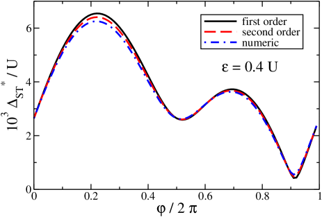
Figure 9: Comparison of the splitting $\Delta_{\rm ST}^{*}$ obtained from the perturbation in first order (full line), Eq. (52), and in the second order (dashed line), Eq. (63) to the exact numerical result (dashed-dotted line), obtained by the direct numerical diagonalization of $H$, Eq. (30). The plots show the splitting $\Delta_{\rm ST}^{*}$ as a function of the angle $\varphi$ for the anticrossing at the detuning $\epsilon^{*}=0.4U$. The parameters used in this plot are $U=1$, $t=0.02$, $V_{+}=0.75$, $V_{-}=0.74$, $\Omega=0.005$, and $\delta{\bf{b}}=(-0.0006,0.0008,0.0012)$.

VII Ratio of spin-orbit and hyperfine terms

As pointed out before, the spin non-conserving Hamiltonian in the vicinity of the anticrossing can be used to get experimental access to the spin orbit interaction and nuclear polarization in the difference-field $\delta{{\bf{b}}}$. Being a function of controllable parameters $\epsilon$ and $\bar{{\bf{b}}}$, this Hamiltonian can be altered by applying voltages to electrodes in the vicinity of the quantum dots, adjusting the strength of an external magnetic field, or changing the direction of the field.

The effect of the competition between spin orbit and hyperfine induced spin flips on the efficiency of angular momentum transfer between electron and nuclear spins was recently studied theoretically, both in the context of dc transport experiments Rudner and Levitov (2010) and in the context of gate-sweep experiments Rudner et al. (2010); Brataas and Rashba (2011). References Rudner and Levitov (2010) and Rudner et al. (2010) revealed striking sensitivities of the polarization transfer efficiency on the ratio of spin orbit and hyperfine coupling strengths. In those works, the coupling strengths were treated as phenomenological parameters. Here we provide explicit expressions for them, and discuss how they can be tuned.

Following the notation of Ref. Rudner et al. (2010) we write

$$v_{\vartheta}=v_{\rm SO}+e^{i\vartheta}v_{\rm HF},$$ (64)

where $v_{\rm SO}$ and $v_{\rm HF}$ stand for the transitions caused by spin orbit and hyperfine interactions, respectively. Comparing with Eq. (48), we can identify $v_{\vartheta}$ with $H_{\rm 34}$. Then, adjusting the overall phase to make the spin-orbit part $v_{\rm SO}$ real, we identify in lowest order

$$v_{\rm SO} =|\Omega\sin\varphi\sin\psi|$$ (65)

$$v_{\rm HF} =|\cos\psi|\sqrt{\left(\delta{\bf{b}}\cdot{\bf{e^{\prime}}}\right)^{2}+\delta b_{y}^{2}},$$ (66)

$$\vartheta =\arctan\left[\frac{-\delta{\bf{b}}\cdot{\bf{e^{\prime}}}}{\delta b_{y}}\right].$$ (67)

The explicit expression for $\vartheta$ shows that the phase of the matrix element can be adjusted not only by changing the direction of $\delta{\bf{b}}$, but also by rotating the external magnetic field, which changes ${\bf{e^{\prime}}}$, and also controls the effective spin-orbit coupling strength.

Our results show that, in principle, it is possible to switch between the two regimes of hyperfine-dominated and spin-orbit-dominated behavior, by changing the external magnetic field strength and direction. In the strong field regime, with sum-field $\bar{{\bf{b}}}$ being large, $\varepsilon^{*}$ is also large, and thus the spin-orbit terms become dominant ($\psi$ approaches $\pi/2$). This behavior is illustrated in Fig. 5. Note that the large values of $\varepsilon^{*}$ require strong $\bar{b}$ fields. On the other hand, switching to the regime $v_{\rm HF}>v_{\rm SO}$ is always possible by rotating the direction of the magnetic field so that it coincides with $\pm\boldsymbol{\Omega}/|\boldsymbol{\Omega}|$ giving $\varphi\approx 0$. In this case, the term $v_{\rm SO}$ is negligible and $v_{\rm HF}$ dominates the splitting. Higher-order corrections to the effective Hamiltonian at the anticrossing point do not alter this basic picture of the splitting, but they do change the values of the parameters $\psi$ and $\varphi$ at which the switching occurs.

The switching between the regimes dominated either by spin orbit or by hyperfine interactions can potentially be achieved as follows. For the regime $v_{\rm SO}>v_{\rm HF}$, the sum-field $\bar{{\bf{b}}}$ should point along the spin orbit field $\boldsymbol{\Omega}$, see Eqs. (26) and (27), in order to maximize $|\sin\varphi|$. Also, the applied field should be as strong as possible, in order to maximize the amplitude of the singlet $|(0,2)S\rangle$ (contributing to the anticrossing singlet $|S_{-}\rangle$, see Eq. (37)). On the other hand, the opposite regime, $v_{\rm HF}>v_{\rm SO}$, can be reached by orienting $\bar{{\bf{b}}}$ along $\boldsymbol{\Omega}$, and thus reaching $\sin\varphi=0$. If $\sin\varphi=0$ cannot be achieved, $v_{\rm SO}$ can be reduced by decreasing $\bar{{\bf{b}}}$ and thereby increasing the amplitude of the singlet state $|(1,1)S\rangle$ in the $|S_{-}\rangle$-singlet at the anticrossing.

VIII Conclusions

We have derived an effective two level Hamiltonian $H_{\rm cr}$ for a detuned two-electron double quantum dot in an external magnetic field. Our effective Hamiltonian describes the dynamics of the electron spins for the values of detuning $\varepsilon\approx\varepsilon^{*}$ close to the anticrossing of the lowest energy $S=0$ and the lowest energy $S=1$ state. We have shown how $H_{\rm cr}$ can be used in the interpretation of experiments that probe electron spin interactions by charge sensing and transport in the Coulomb blockade regime. The dependence of $H_{\rm cr}$ on the detuning and magnetic fields can also be used to switch the spin dynamics in a double quantum dot between the spin-orbit dominated regime, and the hyperfine-dominated regime.

The spin dynamics at the anticrossing is governed by the spin-orbit and nuclear hyperfine interactions. In a double quantum dot, these two interactions act differently on the orbital electronic states. On one hand, the spin-orbit interaction causes hopping of an electron between the quantum dots accompanied by a spin rotation, thus changing the occupation of the quantum dots. On the other hand, the nuclear hyperfine interaction acts as an inhomogeneous magnetic field, and causes spin rotations that are local to the dots, leaving the charge state unchanged. Due to this distinction, the detuning $\varepsilon$ controls the relative strength of the two interactions in $H_{\rm cr}$, in addition to the ratio $|\Omega|/|\delta{\bf{b}}|$, or $|\Omega|/\sigma$. In the limit of detuning much stronger than the on-site repulsion of the dots, $\varepsilon\gg U$, $H_{\rm cr}$ describes mostly the spin-orbit interaction, with negligible hyperfine effects. In the case of weaker detuning, the effective hyperfine interactions can be of the size comparable to the effective spin orbit interactions.

In addition, we find that the orientations of both the double quantum dot and the external magnetic field, described in the $H_{\rm cr}$ by the spin-orbit field $\boldsymbol{\Omega}$ and the sum field $\bar{{\bf{b}}}$, influence the effective spin orbit interaction. In particular, by having $\bar{{\bf{b}}}$ pointing along $\boldsymbol{\Omega}$, we can suppress the spin orbit effects completely (in leading order).

The splitting of the anticrossing states is accessible to experiments. It can be calculated from $H_{\rm cr}$, and we find the dependence of this splitting on detuning and the strength and direction of the sum field, $\Delta_{\rm ST}(\varepsilon,\bar{b},\varphi)$. Of particular interest is the splitting of levels at the anticrossing. We calculate this quantity, $\Delta^{*}_{\rm ST}(\varepsilon^{*},\varphi)$, as a function of the detuning at the anticrossing point, $\varepsilon^{*}$, and the orientation of the sum field, given by the angle $\varphi$. Both the spin orbit interaction strength and the inhomogeneity in the hyperfine coupling can be deduced by measuring the splitting and using our formulas for $\Delta^{*}_{\rm ST}(\varepsilon^{*},\varphi)$.

The relative strength of the spin orbit and hyperfine terms in $H_{\rm cr}$ has a profound effect on the coupled dynamics of electron and nuclear spins. The value of the average angular momentum transfer to nuclear spins as an electron tunnels through a spin-blockaded DQD changes sharply as the interaction goes from the spin-orbit-dominated to the hyperfine-dominated regime. The spin orbit interaction is dominant in the limit of strong detuning $\varepsilon^{*}\gg U-V_{+}$. The regime dominated by nuclear hyperfine interaction is reached when the detuning is weaker $\varepsilon^{*}\lesssim t$ and the orientation of the sum field is along $\boldsymbol{\Omega}$. Using the dependencies of the matrix elements on gate voltages and magnetic field strength and orientation, it may be possible to tune between these two regimes in situ, thus enabling experiments to study their sensitive competition.

Acknowledgements We gratefully acknowledge helpful discussions with Izhar Neder. This work is partially supported by the Swiss NSF, NCCR Nanoscience and QSIT, DARPA QuEST, and the Intelligence Advanced Research Projects Activity (IARPA) through the Army Research Office.

References

- Loss and DiVincenzo (1998) D. Loss and D. P. DiVincenzo, Phys. Rev. A 57, 120 (1998).
- Hanson et al. (2007) R. Hanson, L. P. Kouwenhoven, J. R. Petta, S. Tarucha, and L. M. K. Vandersypen, Rev. Mod. Phys. 79, 1217 (2007).
- Żak et al. (2010) R. A. Żak, B. Röthlisberger, S. Chesi, and D. Loss, Rivista del Nuovo Cimento 033, 345 (2010).
- Benjamin (2001) S. C. Benjamin, Phys. Rev. A 64, 054303 (2001).
- Levy (2002) J. Levy, Phys. Rev. Lett. 89, 147902 (2002).
- Wu and Lidar (2002) L.-A. Wu and D. A. Lidar, Phys. Rev. A 66, 062314 (2002).
- Stepanenko and Bonesteel (2004) D. Stepanenko and N. E. Bonesteel, Phys. Rev. Lett. 93, 140501 (2004).
- Golovach et al. (2006) V. N. Golovach, M. Borhani, and D. Loss, Phys. Rev. B 74, 165319 (2006).
- Koppens et al. (2006) F. H. L. Koppens, C. Buizert, K. J. Tielrooij, I. T. Vink, K. C. Nowack, T. Meunier, K. L. P., and V. L. M. K., Nature 442, 766 (2006).
- Nowack et al. (2007) K. C. Nowack, F. H. L. Koppens, Y. V. Nazarov, and L. M. K. Vandersypen, Science 318, 1430 (2007).
- Barthel et al. (2009) C. Barthel, D. J. Reilly, C. M. Marcus, M. P. Hanson, and A. C. Gossard, Phys. Rev. Lett. 103, 160503 (2009).
- Foletti et al. (2009) S. Foletti, H. Bluhm, D. Mahalu, V. Umansky, and A. Yacoby, Nat. Phys 5, 903 (2009).
- Nadj-Perge et al. (2010a) S. Nadj-Perge, S. M. Frolov, E. P. A. M. Bakkers, and L. P. Kouwenhoven, Nature 468, 1084 (2010a).
- Ono et al. (2002) K. Ono, D. G. Austing, Y. Tokura, and S. Tarucha, Science 297, 1313 (2002).
- Johnson et al. (2005) A. C. Johnson, J. R. Petta, C. M. Marcus, M. P. Hanson, and A. C. Gossard, Phys. Rev. B 72, 165308 (2005).
- Tarucha et al. (2006) S. Tarucha, Y. Kitamura, T. Kodera, and K. Ono, physica status solidi (b) 243, 3673 (2006).
- Nadj-Perge et al. (2010b) S. Nadj-Perge, S. M. Frolov, J. W. W. van Tilburg, J. Danon, Y. V. Nazarov, R. Algra, E. P. A. M. Bakkers, and L. P. Kouwenhoven, Phys. Rev. B 81, 201305 (2010b).
- Rudner and Levitov (2010) M. S. Rudner and L. S. Levitov, Phys. Rev. B 82, 155418 (2010).
- Rudner et al. (2010) M. S. Rudner, I. Neder, L. S. Levitov, and B. I. Halperin, Phys. Rev. B 82, 041311 (2010).
- Brataas and Rashba (2011) A. Brataas and E. I. Rashba, Phys. Rev. B 84, 045301 (2011).
- Burkard et al. (1999) G. Burkard, D. Loss, and D. P. DiVincenzo, Phys. Rev. B 59, 2070 (1999).
- Overhauser (1953) A. W. Overhauser, Phys. Rev. 92, 411 (1953).
- Schliemann et al. (2003) J. Schliemann, A. Khaetskii, and D. Loss, J. Phys.: Condens. Matter 50, R1809 (2003).
- Rashba (1960) E. L. Rashba, Sov. Phys. Solid State (1960).
- Bychkov and Rashba (1984) Y. Bychkov and E. Rashba, J. Phys. C 17, 6039 (1984).
- Dyakonov and Kachorovskii (1986) M. Dyakonov and V. Kachorovskii, Sov. Phys. Semicond. 20, 110 (1986).
- Dresselhaus (1955) G. Dresselhaus, Phys. Rev. 100, 580 (1955).
- Stepanenko et al. (2003) D. Stepanenko, N. E. Bonesteel, D. P. DiVincenzo, G. Burkard, and D. Loss, Phys. Rev. B 68, 115306 (2003).
- Golovach et al. (2008) V. N. Golovach, A. Khaetskii, and D. Loss, Phys. Rev. B 77, 045328 (2008).
- Reilly et al. (2008a) D. J. Reilly, J. M. Taylor, J. R. Petta, C. M. Marcus, M. P. Hanson, and A. C. Gossard, Science 321, 817 (2008a).
- Reilly et al. (2008b) D. J. Reilly, J. M. Taylor, E. A. Laird, J. R. Petta, C. M. Marcus, M. P. Hanson, and A. C. Gossard, Phys. Rev. Lett. 101, 236803 (2008b).
- Bluhm et al. (2010) H. Bluhm, S. Foletti, D. Mahalu, V. Umansky, and A. Yacoby, Phys. Rev. Lett. 105, 216803 (2010).
- Schroer et al. (2011) M. D. Schroer, K. D. Petersson, M. Jung, and J. R. Petta, Phys. Rev. Lett. 107, 176811 (2011).
- Zumbühl et al. (2002) D. M. Zumbühl, J. B. Miller, C. M. Marcus, K. Campman, and A. C. Gossard, Phys. Rev. Lett. 89, 276803 (2002).
- Petta et al. (2008) J. R. Petta, J. M. Taylor, A. C. Johnson, A. Yacoby, M. D. Lukin, C. M. Marcus, M. P. Hanson, and A. C. Gossard, Phys. Rev. Lett. 100, 067601 (2008).
- Schrieffer and Wolff (1966) J. R. Schrieffer and P. A. Wolff, Phys. Rev. 149, 491 (1966).
- Bravyi et al. (2011) S. Bravyi, D. P. DiVincenzo, and D. Loss, Annals of Physics 326, 2793 (2011).