Eigenvalue problems, spectral parameter power series, and modern applications

Abstract

Our review is dedicated to a wide class of spectral and transmission problems arising in different branches of applied physics. One of the main difficulties in studying and solving eigenvalue problems for operators with variable coefficients consists in obtaining a corresponding dispersion relation or characteristic equation of the problem in a sufficiently explicit form. Solutions of the dispersion relation are the eigenvalues of the problem. When the dispersion relation is known the eigenvalues are found numerically even for relatively simple problems with constant coefficients because even in those cases as a rule the dispersion relation represents a transcendental equation the exact solutions of which are unknown.

In the present review we deal with the recently introduced method of spectral parameter power series (SPPS) and show how its application leads to an explicit form of the characteristic equation for different eigenvalue problems involving Sturm-Liouville equations with variable coefficients. We consider Sturm-Liouville problems on finite intervals; problems with periodic potentials involving the construction of Hill’s discriminant and Floquet-Bloch solutions; quantum-mechanical spectral and transmission problems as well as the eigenvalue problems for the Zakharov-Shabat system. In all these cases we obtain a characteristic equation of the problem which in fact reduces to finding zeros of an analytic function given by its Taylor series. We illustrate the application of the method with several numerical examples which show that at present the SPPS method is the easiest in the implementation, the most accurate and efficient. We emphasize that the SPPS method is not a purely numerical technique. It gives an analytical representation both for the solution and for the characteristic equation of the problem. This representation can be approximated by different numerical techniques and for practical purposes constitutes a powerful numerical method but most importantly it offers additional insight into the spectral and transmission problems.

Keywords: spectral parameter power series; Sturm-Liouville problems; dispersion relations; periodic potentials; Hill’s discriminant; supersymmetry; Zakharov-Shabat system

1 Introduction

Solution of second-order linear differential equations belongs to a classical field of mathematics in which as an overwhelming majority of its users from students to active researchers believe that everything that was possible to do theoretically is essentially done, and whatever the analysts invent, in the domain of practical solution of equations and related models anyway the numerical discrete schemes more and more refined due to the massive efforts of experts in numerical analysis and computer sciences will be more accurate and efficient. For the good luck of mathematics and its applications a considerable number of analysts as well as of advanced users of mathematical methods in physics are aware of many strong limitations in applicability of available numerical schemes. For examples, if the discrete spectrum of a problem is not necessarily real, practically the whole machinery of advanced numerical techniques does not apply bringing to the surface in fact one option only: finite differences. The importance of this technique lies in its universality. Nevertheless it usually gives way to many other approaches whenever they become applicable. The main difficulty in finding complex eigenvalues is due to the fact that the universally used shooting method works if only there is a clear criterion for choosing every next shot. Meanwhile the real numbers is an ordered set and zero is located always between a negative and a positive outcomes of the corresponding shots, the complex plane does not admit such a simple rule. There are many other situations (even when the eigenvalues are real) when the shooting procedure finds considerable difficulties and at the same time the method of finite differences is not applicable at all. For example, when the spectral parameter participates in the boundary conditions. Such situation in fact is more common in applications than otherwise.

In the present review we discuss an approach developed in the last few years and called the spectral parameter power series (SPPS) method. It is important to notice that the SPPS method is not merely another numerical technique. On the contrary, it is an analytical approach giving new analytical results and at the same time lending itself to numerical calculation. The SPPS method allows one to obtain two linearly independent solutions of the Sturm-Liouville equation (in Section 2 we specify the conditions imposed on the coefficients)

$$(pu^{\prime})^{\prime}+qu=\lambda ru$$ (1)

in the form

$$u_{1}(x)=\sum\limits_{k=0}^{\infty}a_{k}(x)\lambda^{k}\quad\text{and}\quad u_{2}(x)=\sum\limits_{k=0}^{\infty}b_{k}(x)\lambda^{k}$$

where $\lambda$ is a spectral parameter and the series are uniformly convergent. Such representations from time to time appear in mathematical literature in different contexts. We mention here [6, Sect. 10] and [28]. The main difference is the form in which the coefficients $a_{k}$ and $b_{k}$, $k=0,1,\ldots$ are represented. In previous works the calculation of the coefficients was proposed in terms of successive integrals with the kernels in the form of iterated Green functions (see [6, Sect. 10]). This makes any computation based on such representation difficult and less practical. Moreover, theoretical study of the corresponding series and their properties becomes considerably more complicated. We show that $a_{k}$ and $b_{k}$ can be calculated in terms of the coefficients $p$ and $r$ of (1) as well as of a particular solution of the equation $(pv^{\prime})^{\prime}+qv=0$. The obtained representations of the coefficients $a_{k}$ and $b_{k}$ are relatively simple and well suited both for theoretical estimates and for numerical computation with a minimum of programmer’s efforts required. Behind this representation of the coefficients $a_{k}$ and $b_{k}$ there is one of the possible factorizations of the operator $L=\frac{d}{dx}p\frac{d}{dx}+q$ sometimes called the Polya factorization (see [53]).

The main advantage of the SPPS method is akin to that of such asymptotic approaches as the WKB method - it allows one to work with an analytical representation of the solution instead of a table of values delivered by a numerical method. This is important from different points of view, often it gives a new physical insight into the problem. The difference between the SPPS and the asymptotic techniques lies in the fact that to apply the SPPS method it is not necessary to assume the smallness or the largeness of the parameter $\lambda$. For example, the WKB approximation can be efficiently applied to (1) when $\lambda$ is sufficiently large which is quite useless when an eigenvalue problem related to (1) is considered.

We show that 1) for solving initial value and boundary value problems the SPPS method performs better or equal in comparison to purely numerical techniques; 2) it is highly advantageous when the solution is required for many different values of the spectral parameter; 3) the SPPS method allows us to write down an explicit form of the characteristic equations for many different spectral problems which in practice reduces the spectral problem to finding zeros of a corresponding analytic function given by its Taylor series. We emphasize that the method is applicable in different situations when some other approaches are unavailable (complex eigenvalues; $\lambda$-dependent boundary conditions, etc.) The method is simple and can be introduced in mathematical courses for physicists.

In Section 2, we review the main results from [62] and [66] concerning the SPPS representation of the solutions of (1) and show that even in solving initial and boundary value problems this technique converted into a simple numerical algorithm is clearly competitive when compared to standard routines for numerical integration of linear ordinary differential equations. In Section 3 we apply the SPPS method to Sturm-Liouville spectral problems with or without the spectral parameter in the boundary conditions. Here together with some results from [66] we present new results concerning the problems admitting complex eigenvalues. Section 4 is dedicated to the spectral problems for periodic potentials. We give an SPPS representation for Hill’s discriminant [55] and show how the SPPS method allows one to construct the Bloch solutions of the problem. In Section 5 we consider two classical problems of mathematical physics: the quantum-mechanical spectral problem and the transmission problem. Following [18] we present a characteristic (dispersion) equation equivalent to the eigenvalue problem for the Schrödinger operator with a potential which is an arbitrary continuous function on a finite interval outside of which it is constant. We discuss some numerical tests as well. The transmission problem is presented in the context of electromagnetic wave propagation as the problem of calculation of the reflection and transmission coefficients for a plane wave which is incident on an inhomogeneous layer under an arbitrary angle of incidence. Following [17] we discuss application of the SPPS method to this problem. Section 6 is dedicated to the eigenvalue problem for the Zakharov-Shabat system. We present the dispersion equation [68] for the problem for a real-valued, finitely supported potential and discuss its practical application. Finally, in Section 7 we make some concluding remarks.

This review is for the colleagues interested in all kinds of problems involving solution of Sturm-Liouville type equations. We hope to attract more attention to the SPPS approach which combines the possibility to work with analytical representations of solutions and of characteristic equations of the problems with simplicity, rapid convergence, and accuracy when used for numerical computation.

2 Spectral parameter power series representation for solutions of the Sturm-Liouville equation

Let us consider the Sturm-Liouville equation

$$(pu^{\prime})^{\prime}+qu=\lambda ru~{},$$ (2)

where $p$, $q$ and $r$ are complex valued functions and $\lambda$ is a complex parameter. The following result [66] gives us a convenient form for a general solution of (2) as a spectral parameter power series.

Theorem 1

[66] Assume that on a finite interval $[a,b]$, equation

$$(pv^{\prime})^{\prime}+qv=0,$$ (3)

possesses a particular solution $u_{0}$ such that the functions $u_{0}^{2}r$ and $1/(u_{0}^{2}p)$ are continuous on $[a,b]$. Then the general solution of (2) on $(a,b)$ has the form

$$u=c_{1}u_{1}+c_{2}u_{2}~{},$$ (4)

where $c_{1}$ and $c_{2}$ are arbitrary complex constants,

$$u_{1}=u_{0}{\displaystyle\sum\limits_{k=0}^{\infty}}\lambda^{k}\widetilde{X}^{(2k)}\quad\text{and}\quad u_{2}=u_{0}{\displaystyle\sum\limits_{k=0}^{\infty}}\lambda^{k}X^{(2k+1)}$$ (5)

with $\widetilde{X}^{(n)}$ and $X^{(n)}$ being defined by the recursive relations

$$\widetilde{X}^{(0)}\equiv 1,\quad X^{(0)}\equiv 1,$$ (6)

$$\widetilde{X}^{(n)}(x)=\left\{\begin{tabular}[c]{ll}${\displaystyle\int\limits_{x_{0}}^{x}}\widetilde{X}^{(n-1)}(s)u_{0}^{2}(s)r(s)\,ds$,&$n$ \text{odd,}\\ ${\displaystyle\int\limits_{x_{0}}^{x}}\widetilde{X}^{(n-1)}(s)\frac{1}{u_{0}^{2}(s)p(s)}\,ds$,&$n$ \text{even,}\end{tabular}\ \ \ \ \ \right.$$ (7)

∫x0xX(n−1)(s)u02(s)r(s)ds,n even,X^{(n)}(x)=\left\{\begin{tabular}[c]{ll}${\displaystyle\int\limits_{x_{0}}^{x}}X^{(n-1)}(s)\frac{1}{u_{0}^{2}(s)p(s)}\,ds$,&$n$ \text{odd,}\\ ${\displaystyle\int\limits_{x_{0}}^{x}}X^{(n-1)}(s)u_{0}^{2}(s)r(s)\,ds$,&$n$ \text{even},\end{tabular}\ \ \ \ \ \ \ \ \right.

∫x0xX(-n1)(s)1u02(s)p(s)ds, n odd, (8)

where $x_{0}$ is an arbitrary point in $[a,b]$ such that $p$ is continuous at $x_{0}$ and $p(x_{0})\neq 0$. Further, both series in (5) converge uniformly on $[a,b]$.

For a detailed proof we refer to [66]. It is based on some simple observations. First of all the knowledge of a particular solution of (3) allows one to factorize the Sturm-Liouville operator $L=\frac{d}{dx}p\frac{d}{dx}+q$ in the form $L=\frac{1}{u_{0}}\frac{d}{dx}\,p\,u_{0}^{2}\frac{d}{dx}\frac{1}{u_{0}}$, also known as the Polya factorization [53] as mentioned before. This form is well suited for establishing how the operator $\frac{1}{r}L$ acts on each member of the series (5). For example, $\frac{1}{r}L\left(u_{0}\widetilde{X}^{(2k)}\right)=u_{0}\widetilde{X}^{(2k-2)}$, $k\in\mathbb{N}$. Analogously, $\frac{1}{r}L\left(u_{0}X^{(2k+1)}\right)=u_{0}X^{(2k-1)}$.

Considering the system of functions $\left\{\varphi_{n}\right\}_{n=0}^{\infty}$ defined as follows $\varphi_{0}=u_{0}$,

$$\varphi_{n}(x)=\left\{\begin{tabular}[c]{ll}$u_{0}(x)X^{(n)}(x)$,&$n$ \text{odd,}\\ $u_{0}(x)\widetilde{X}^{(n)}(x)$,&$n$ \text{even,}\end{tabular}\ \ \ \ \ \ \ \ \ \ \ \ \right.\$$ (9)

we find that $\frac{1}{r}L\varphi_{0,1}=0$ and $\frac{1}{r}L\varphi_{n}=\varphi_{n-2}$, $n=2,3,\ldots$. These properties are characteristic for the so-called $L$-bases (introduced in [34], unfortunately this important book has not been translated into English), and hence formulas (6)-(8) represent a practical way to calculate an $L$-basis. In [64] it was established that the system of functions $\left\{\varphi_{n}\right\}_{n=0}^{\infty}$ is complete in $L_{2}(a,b)$. For further related properties we refer to [65].

To establish the uniform convergence of the series in (5) as well as to get a rough but useful estimate for the velocity of their convergence it is sufficient to observe that

$$\left|\widetilde{X}^{(2k)}\right|\leq\left(\max\left|ru_{0}^{2}\right|\right)^{k}\left(\max\left|\frac{1}{pu_{0}^{2}}\right|\right)^{k}\frac{\left|b-a\right|^{2k}}{\left(2k\right)!}$$ (10)

(a similar inequality is available for $\left|X^{(2k+1)}\right|$ as well). Thus, the series ${\displaystyle\sum\limits_{k=0}^{\infty}}\lambda^{k}\widetilde{X}^{(2k)}$ is majorized by a convergent numerical series ${\displaystyle\sum\limits_{k=0}^{\infty}}\frac{c^{k}}{\left(2k\right)!}$ with $c=\left|\lambda\right|\left(\max\left|ru_{0}^{2}\right|\right)\left(\max\left|\frac{1}{pu_{0}^{2}}\right|\right)\left|b-a\right|^{2}$.

It is worth noticing that from (5) it is easy to obtain that $u_{1}$ and $u_{2}$ satisfy the following initial conditions

$$u_{1}(x_{0})=u_{0}(x_{0}),\qquad u_{1}^{\prime}(x_{0})=u_{0}^{\prime}(x_{0}),$$ (11)

$$u_{2}(x_{0})=0,\qquad u_{2}^{\prime}(x_{0})=\frac{1}{u_{0}(x_{0})p(x_{0})}.$$ (12)

Remark 2

The possibility mentioned in the Introduction to represent solutions of the Sturm-Liouville equation in the form of spectral parameter power series is by no means a novelty, though it is not a widely used tool. In fact, besides the work reviewed below we are able to mention only [6, Sect. 10], [28] and the recent paper [61]) and to the best of our knowledge it was applied for the first time for solving spectral problems in [66]. The reason of this underuse of the SPPS lies in the form in which the expansion coefficients were sought. Indeed, in previous works the calculation of coefficients was proposed in terms of successive integrals with the kernels in the form of iterated Green functions (see [6, Sect. 10]). However, this makes any computation based on such representation difficult, less practical, and even proofs of the most basic results like, e.g., the uniform convergence of the spectral parameter power series for any value of $\lambda\in\mathbb{C}$ (established in Theorem 1) are not an easy task. For example, in [6, p. 16] the parameter $\lambda$ is assumed to be small and no proof of convergence is given. Moreover, in [11] a discrete analogue of Theorem 1 together with some further applications to Jacobi operators were established and it was pointed out that as well as in the continuous case the SPPS representation for solutions of the Jacobi operators was considered as a perturbation technique, however, even the situation with the convergence of such series was not satisfactorily understood. We recommend the book [2] where the possibility of divergence of such series as those considered in the present work is assumed. Due to the representation of the expansion coefficients similar to (7), (8), it was shown in [11] that the series are not only convergent but in the discrete case they are actually finite sums.

The way of how the expansion coefficients in (5) are calculated according to (7) and (8) is relatively simple and straightforward. This is why the estimation of the rate of convergence of the series (5) presents no difficulty, see (10). Another crucial feature of the introduced representation of the expansion coefficients in (5) consists in the fact that as we repeatedly observe in subsequent pages not only the expansion coefficients themselves also denoted by $\varphi_{n}$ in (9) are necessary in solving different spectral problems related to the Sturm-Liouville equation but also the formal powers apparently obtained as a by-product of the recursive integration procedure (7) and (8), namely the functions $\widetilde{X}^{(2k+1)}$ and $X^{(2k)}$, $k=0,1,2,\ldots$, which do not participate explicitly in the representation of solutions (5), naturally appear in dispersion equations corresponding to the spectral problems. See (22) and (23) for the dispersion equations equivalent to the classical Sturm-Liouville eigenvalue problem, (39) for the SPPS representation of the Hill discriminant, (61) for the dispersion equation equivalent to the quantum-mechanical eigenvalue problem on the whole axis or (88) for the dispersion equation equivalent to the Zakharov-Shabat eigenvalue problem.

The consideration of formal powers (7) and (8) as infinite families of functions intimately related to the corresponding Sturm-Liouville operator led in [12], [13] and [67] to a deeper understanding of the transmutation operators [5], [14] also known as transformation operators [72], [77]. Indeed, the functions $\varphi_{n}(x)$ resulted to be the images of the powers $x^{n}$ under the action of a corresponding transmutation operator [13]. This makes it possible to apply the transmutation operator even when the operator itself is unknown (and this is the usual situation - there are very few explicitly constructed examples available) due to the fact that its action on any polynomial is known. This result was used in [12] and [13]  to prove the completeness (Runge-type approximation theorems) for families of solutions of two-dimensional Schrödinger and Dirac equations with variable complex-valued coefficients.

Remark 3

One of the functions $ru_{0}^{2}$ or $1/(pu_{0}^{2})$ may not be continuous on $[a,b]$ and yet $u_{1}$ or $u_{2}$ may make sense. For example, in the case of the Bessel equation $(xu^{\prime})^{\prime}-\frac{1}{x}u=-\lambda xu,$ we can choose $u_{0}(x)=x/2.$ Then $1/(pu_{0}^{2})\notin C[0,1]$. Nevertheless, all integrals (7) exist and $u_{1}$ coincides with the nonsingular $\left(1/\sqrt{\lambda}\right)J_{1}(\sqrt{\lambda}x)$, while $u_{2}$ is a singular solution of the Bessel equation.

Remark 4

When $p$ and $q$ are real-valued, $p(x)\neq 0$ for all $x\in[a,b]$ and $p$, $p^{\prime}$, $q$ are continuous functions on $[a,b]$, the equation

$$Lv=0$$ (13)

is a regular Sturm-Liouville equation and possesses two linearly independent real valued solutions $v_{1}$ and $v_{2}$. Due to Sturm’s separation theorem (see, e.g., [57, p. 10]) their zeros occur alternately and hence $u_{0}=v_{1}+iv_{2}$ can be chosen as the required in theorem 1 particular solution. If $r$ is a continuous on $[a,b]$ (in general, complex-valued) function then the conditions of theorem 1 are fulfilled.

The solutions $v_{1}$ and $v_{2}$ from Remark 4 can be in fact calculated using the same procedure from Theorem 1. Indeed, consider equation (13) which can be written in the form

$$(pv^{\prime})^{\prime}=-qv.$$

It has the form (2) with $r:=-q$, $\lambda=1$ and with a convenient solution $v_{0}\equiv 1$ of the (homogeneous) equation $(pv_{0}^{\prime})^{\prime}=0$. Application of theorem 1 gives us the following two linearly independent solutions of (13),

$$v_{1}={\displaystyle\sum\limits_{k=0}^{\infty}}\widetilde{Y}^{(2k)}\quad\text{and}\quad v_{2}={\displaystyle\sum\limits_{n=0}^{\infty}}Y^{(2k+1)}$$ (14)

where

$$\widetilde{Y}^{(0)}\equiv 1,\quad Y^{(0)}\equiv 1,$$ (15)

$$\widetilde{Y}^{(n)}(x)=\left\{\begin{tabular}[c]{ll}$-{\displaystyle\int\limits_{x_{0}}^{x}}\widetilde{Y}^{(n-1)}(s)q(s)\,ds$,&$n$ \text{odd,}\\ ${\displaystyle\int\limits_{x_{0}}^{x}}\widetilde{Y}^{(n-1)}(s)\frac{1}{p(s)}\,ds$,&$n$ \text{even,}\end{tabular}\ \ \ \ \ \ \ \right.$$ (16)

$$Y^{(n)}(x)=\left\{\begin{tabular}[c]{ll}${\displaystyle\int\limits_{x_{0}}^{x}}Y^{(n-1)}(s)\frac{1}{p(s)}\,ds$,&$n$ \text{odd,}\\ $-{\displaystyle\int\limits_{x_{0}}^{x}}Y^{(n-1)}(s)q(s)\,ds$,&$n$ \text{even},\end{tabular}\ \ \ \ \ \ \ \ \ \ \right.$$ (17)

and the series in the equalities for $v_{1}$ and $v_{2}$ converge uniformly on $[a,b]$.

Note that

$$v_{1}(x_{0})=1,\quad v_{1}^{\prime}(x_{0})=0,\quad v_{2}(x_{0})=0,\quad v_{2}^{\prime}(x_{0})=1/p(x_{0}).$$

Solutions of (13) in the form (14) is a long known result (see, e.g., [100]).

Before we proceed to discuss eigenvalue and scattering problems it is worth noticing that the representation of a general solution of the Sturm-Liouville equation in the form of a spectral parameter power series (SPPS) given by theorem 1 represents a natural and highly competitive method for numerical solution of initial and boundary value problems. Compared to the best standard routines it performs better or equal and with minimal programmer’s efforts. Moreover, the advantages of using SPPS become even more transparent when the solution of the problem is required for many different values of the spectral parameter. In such case the auxiliary functions $X^{(n)}$ and $\widetilde{X}^{(n)}$, $n=0,1,2,\ldots$ should be computed only once and then substitution of values of $\lambda$ into the expressions (5) gives us a solution of equation (2) for as many different values of the spectral parameter as needed at no additional computational cost. Nevertheless, first, let us show how SPPS performs at the terrain of numerical ODE solvers for solution of initial value problems. In [17] we made use of Matlab 7 and as a first step compared our results with standard Matlab ODE solvers [3], [92], especially with ode45 which in the considered examples gave always better results than other similar programs. Here we give two examples from [17].

For numerical approximations we consider partial sums of the infinite series (5) and (14), e.g., $u_{1}=u_{0}{\displaystyle\sum\limits_{k=0}^{N}}\lambda^{k}\widetilde{X}^{(2k)}$ and $u_{2}=u_{0}{\displaystyle\sum\limits_{k=0}^{N}}\lambda^{k}X^{(2k+1)}$.  The algorithm was implemented in MATLAB. For the recursive integration we have chosen the following strategy. On each step the integrand is represented through a cubic spline using the spapi routine and the integration is performed using the fnint routine (both from the spline toolbox of MATLAB).

Consider the following initial value problem for (13): $p\equiv 1$, $q\equiv c^{2}$, $v(0)=1$, $v^{\prime}(0)=-1$ on the interval $(0,1)$. For $c=1$ the absolute error of the result calculated by ode45 (with an optimal tolerance chosen) was of order $10^{-9}$ and the relative error was of order $10^{-6}$ whereas the absolute error of the result calculated with the aid of the SPPS representation with $N$ from $55$ to $58$ was of order $10^{-16}$ and the relative error was of order $10^{-14}$. Taking $c=10$ under the same conditions the absolute and the relative errors of ode45 were of order $10^{-6}$ and $10^{-5}$ respectively meanwhile our algorithm gave values of order $10^{-12}$ in both cases. For the initial value problem: $p\equiv-1$, $q\equiv c^{2}$, $v(0)=1$, $v^{\prime}(0)=-1$ on the interval $(0,1)$ in the case $c=1$ the absolute and the relative errors of ode45 were of order $10^{-8}$ whereas in our method this value was of order $10^{-15}$ already for $N=50$. For $c=10$ the absolute and the relative errors of ode45 were of order $10^{-3}$ and $10^{-7}$ respectively and in the case of our method these values were of order $10^{-11}$ and $10^{-14}$ for $N=50$.

Consider yet another example. Let $p\equiv-1$, $q(x)=c^{2}x^{2}+c$  in (13). In this case the general solution has the form

$$v(x)=e^{cx^{2}/2}\left(c_{1}+c_{2}\int_{0}^{x}e^{-ct^{2}}dt\right).$$

Take the same initial conditions as before, $v(0)=1$, $v^{\prime}(0)=-1$. Then, while for $c=1$ the absolute and the relative error of ode45 were both of order $10^{-8}$ and for $c=30$ the absolute error was $0.28$ and the relative error was of order $10^{-6}$, our algorithm ($N=58$) gave the absolute and relative errors of order $10^{-15}$ for $c=1$ and the absolute and relative errors of order $10^{-9}$ and $10^{-15}$ respectively for $c=30.$ All calculations were performed on a common PC with the aid of Matlab 7.

The results of our numerical experiments show that in fact the SPPS representations offer a powerful method for numerical solution of initial value and boundary value problems for linear ordinary differential second-order equations. The numerical calculation of the involved integrals does not represent any considerable difficulty and can be done with a remarkable accuracy.

Another observation which can be of use in many different situations is that if for some purposes a derivative of the solution of (2) is required there is no need to apply to the obtained solution an algorithm for numerical differentiation. Instead, it is easy to see that

$$u_{1}^{\prime}=\frac{u_{0}^{\prime}}{u_{0}}u_{1}+\frac{1}{u_{0}p}{\displaystyle\sum\limits_{k=1}^{\infty}}\lambda^{k}\widetilde{X}^{(2k-1)}\quad\text{and\quad}u_{2}^{\prime}=\frac{u_{0}^{\prime}}{u_{0}}u_{2}+\frac{1}{u_{0}p}{\displaystyle\sum\limits_{k=0}^{\infty}}\lambda^{k}X^{(2k)}.$$ (18)

Thus, the calculated auxiliary functions $X^{(n)}$ and $\widetilde{X}^{(n)}$, $n=0,1,2,\ldots$ are used once more, this time for obtaining the derivative of the solution.

3 Solution of Sturm-Liouville problems

In this section we outline the main ideas behind the application of the SPPS method to the solution of Sturm-Liouville eigenvalue problems referring the interested reader to [66] for additional details and numerical examples. The SPPS method allows one to reduce the Sturm-Liouville problem to the problem of finding zeros of an analytic function of the complex variable $\lambda$. Numerically the problem is reduced to finding roots of a polynomial in $\lambda$. To find the precise expressions for Taylor coefficients of that analytic function let us consider the general Sturm-Liouville problem with unmixed boundary conditions. Thus, we look for the eigenvalues and eigenfunctions of the problem

$$(pu^{\prime})^{\prime}+qu=\lambda ru,$$ (19)

$$u(a)\cos\alpha+u^{\prime}(a)\sin\alpha=0,$$ (20)

$$u(b)\cos\beta+u^{\prime}(b)\sin\beta=0~{},$$ (21)

where $[a,b]$ is a finite segment of the $x$-axis, $\alpha$ and $\beta$ are arbitrary real numbers.

Let us choose the point $x_{0}$ from theorem 1 being equal to $a$ and consider the solutions $u_{1}$ and $u_{2}$ of (19) defined by (5). Then from (11) and (12) we obtain that a linear combination $u=c_{1}u_{1}+c_{2}u_{2}$ satisfies the following conditions at $a$:

$$u(a)=c_{1}u_{0}(a)\quad\text{and\quad}u^{\prime}(a)=c_{1}u_{0}^{\prime}(a)+c_{2}/(u_{0}(a)p(a)).$$

Thus, in order that $u$ satisfy (20), the constants $c_{1}$ and $c_{2}$ must satisfy the equation

$$c_{1}(u_{0}(a)\cos\alpha+u_{0}^{\prime}(a)\sin\alpha)+c_{2}\frac{\sin\alpha}{u_{0}(a)p(a)}=0,$$

which gives $c_{2}=\gamma c_{1}$ when $\alpha\neq\pi n$, with $\gamma=-u_{0}(a)p(a)(u_{0}(a)\cot\alpha+u_{0}^{\prime}(a))$, whereas $c_{1}=0$ when $\alpha=\pi n.$ In the latter case we have that if an eigenfunction of the problem for a given $\lambda$ exists, up to a multiplicative constant it must have a form $u=u_{2}$. The second boundary condition (21) together with (18) leads to the following characteristic equation for the eigenvalues

$$\cos\beta\,u_{0}(b){\displaystyle\sum\limits_{k=0}^{\infty}}\lambda^{k}X^{(2k+1)}(b)+\sin\beta\,\left(u_{0}^{\prime}(b){\displaystyle\sum\limits_{k=0}^{\infty}}\lambda^{k}X^{(2k+1)}(b)+\frac{1}{u_{0}(b)p(b)}{\displaystyle\sum\limits_{k=0}^{\infty}}\lambda^{k}X^{(2k)}(b)\right)=0~{},$$

which is the same to

$${\displaystyle\sum\limits_{k=0}^{\infty}}\lambda^{k}\left(X^{(2k+1)}(b)\left(\cos\beta\,u_{0}(b)+\sin\beta\,u_{0}^{\prime}(b)\right)+\frac{\sin\beta}{u_{0}(b)p(b)}X^{(2k)}(b)\right)=0.$$ (22)

Thus, the Sturm-Liouville problem (19)-(21) in the case $\alpha=\pi n$ reduces to find zeros of the analytic function ${\displaystyle\sum\limits_{k=0}^{\infty}}a_{k}\lambda^{k}$ where the Taylor coefficients $a_{k}$ have the form $a_{k}=X^{(2k+1)}(b)\left(\cos\beta\,u_{0}(b)+\sin\beta\,u_{0}^{\prime}(b)\right)+\frac{\sin\beta}{u_{0}(b)p(b)}X^{(2k)}(b)$.

Now let us suppose $\alpha\neq\pi n$. Then the boundary condition (21) implies that

$$\left(u_{0}(b)\cos\beta+u_{0}^{\prime}(b)\sin\beta\right)\left({\displaystyle\sum\limits_{k=0}^{\infty}}\lambda^{k}\widetilde{X}^{(2k)}(b)+\gamma{\displaystyle\sum\limits_{k=0}^{\infty}}\lambda^{k}X^{(2k+1)}(b)\right)$$

$$+\frac{\sin\beta}{u_{0}(b)p(b)}\left({\displaystyle\sum\limits_{k=1}^{\infty}}\lambda^{k}\widetilde{X}^{(2k-1)}(b)+\gamma{\displaystyle\sum\limits_{k=0}^{\infty}}\lambda^{k}X^{(2k)}(b)\right)=0.$$ (23)

Thus the spectral problem (2), (20), (21) reduces to the problem of calculating zeros of the analytic function $\kappa(\lambda)={\displaystyle\sum\limits_{m=0}^{\infty}}a_{m}\lambda^{m}$ where

$$a_{0}=\left(u_{0}(b)\cos\beta+u_{0}^{\prime}(b)\sin\beta\right)(1+\gamma X^{(1)}(b))+\frac{\gamma\sin\beta}{u_{0}(b)p(b)}$$

and

$$a_{m}=\left(u_{0}(b)\cos\beta+u_{0}^{\prime}(b)\sin\beta\right)\left(\widetilde{X}^{(2m)}(b)+\gamma X^{(2m+1)}(b)\right)$$

$$+\frac{\sin\beta}{u_{0}(b)p(b)}\left(\widetilde{X}^{(2m-1)}(b)+\gamma X^{(2m)}(b)\right),\quad m=1,2,\ldots.$$

This reduction of a Sturm-Liouville spectral problem to finding zeros of an analytic function given by its Taylor series lends itself to a simple numerical implementation. To calculate the first $n$ eigenvalues we consider the Taylor polynomial $\kappa_{N}(\lambda)={\displaystyle\sum\limits_{m=0}^{N}}a_{m}\lambda^{m}$ with $N\geq n$. Thus the numerical approximation of eigenvalues of the Sturm-Liouville problem reduces to the calculation of roots of the polynomial $\kappa_{N}(\lambda)$.

In many physical applications (see [7, 20, 23, 26, 41, 99] and references therein) the Sturm-Liouville problems with boundary conditions dependent on the spectral parameter arise. In this case together with equation (19) and boundary condition (20) the eigenfunction must satisfy a second boundary condition of the form

$$\beta_{1}u(b)-\beta_{2}u^{\prime}(b)=\varphi(\lambda)\left(\beta_{1}^{\prime}u(b)-\beta_{2}^{\prime}u^{\prime}(b)\right),$$ (24)

where $\varphi$ is a complex-valued function of the variable $\lambda$ and $\beta_{1}$, $\beta_{2}$, $\beta_{1}^{\prime}$, $\beta_{2}^{\prime}$ are complex numbers. For some special forms of the function $\varphi$ such as $\varphi(\lambda)=\lambda$ or $\varphi(\lambda)=\lambda^{2}+c_{1}\lambda+c_{2}$, results were obtained [23], [99] concerning the regularity of the problem (19), (20), (24); we will not dwell upon the details. In general, the presence of the spectral parameter in boundary conditions introduces additional considerable difficulties both in theoretical and numerical analysis of the problems. Nevertheless the SPPS approach gives a simple and natural insight into the problem, and its practical application for numerical calculations is not in fact more difficult than in the previously considered situation of $\lambda$-independent boundary conditions.

For simplicity, let us suppose that $\alpha=0$ and hence the condition (20) becomes $u(a)=0$. Then as was shown above, if an eigenfunction exists it necessarily coincides with $u_{2}$ up to a multiplicative constant. In this case condition (24) becomes equivalent to the equality [66]

$$\left(u_{0}(b)\varphi_{1}(\lambda)-u_{0}^{\prime}(b)\varphi_{2}(\lambda)\right){\displaystyle\sum\limits_{k=0}^{\infty}}\lambda^{k}X^{(2k+1)}(b)-\frac{\varphi_{2}(\lambda)}{u_{0}(b)p(b)}{\displaystyle\sum\limits_{k=0}^{\infty}}\lambda^{k}X^{(2k)}(b)=0~{},$$ (25)

where $\varphi_{1,2}(\lambda)=\beta_{1,2}-\beta_{1,2}^{\prime}\varphi(\lambda)$. Calculation of eigenvalues given by (25) is especially simple in the case of $\varphi$ being a polynomial of $\lambda$. Precisely this particular situation was considered in all of the above-mentioned references concerning Sturm-Liouville problems with spectral parameter dependent boundary conditions. In any case the knowledge of an explicit characteristic equation (25) for the spectral problem (19), (20), (24) makes possible its accurate and efficient solution.

The paper [66] contains several numerical tests corresponding to a variety of computationally difficult problems. All they reveal an excellent performance of the SPPS method. We do not review them here referring the interested reader to [66]. Instead we consider another interesting example, a Sturm-Liouville problem admitting complex eigenvalues.

Consider the equation (2) with $p\equiv-1$, $q\equiv 0$ and $r\equiv 1$ on the interval $(0,\pi)$ with the boundary conditions $u(0)=0$ and $u(\pi)=-\lambda^{2}u(\pi)$. The exact eigenvalues of the problem are $\lambda_{n}=n^{2}$ together with the purely imaginary numbers $\lambda_{\pm}=\pm i$. Application of the SPPS method with $N=100$ and $3000$ interpolating points (used for representing the integrands as splines) delivered the following results $\lambda_{1}=1$, $\lambda_{2}=4.0000000000007$, $\lambda_{3}=9.00000000001$, $\lambda_{4}=15.99999999996$, $\lambda_{5}=25.000000002$, $\lambda_{6}=35.99999997$, $\lambda_{7}=49.0000004$, $\lambda_{8}=63.9999994$, $\lambda_{9}=80.9996$, $\lambda_{10}=100.02$ and $\lambda_{\pm}=\pm i$. Thus, the complex eigenvalues are as easily and accurately detected by the SPPS method as the real eigenvalues. Note that for a better accuracy in calculation of higher eigenvalues of a Sturm-Liouville problem an additional simple shifting procedure (described in [66]) based on the representation of solutions of (2) not as a series in powers of $\lambda$ but in powers of $(\lambda-\lambda_{0})$ is helpful. We did not apply it here and hence the accuracy of the calculated value of $\lambda_{10}$ is considerably worse than the accuracy of the first calculated eigenvalues which in general can be improved by means of the mentioned shifting procedure.

4 Periodic potentials: Floquet-Bloch solutions and Hill’s discriminant

Towards the end of the 19th century, Hill [46] and Floquet [38] initiated the rigorous study of the spectral properties of periodic Sturm-Liouville equations with real coefficients and with periodic (and antiperiodic) conditions imposed to their solutions $\mathbf{y}(0)=\pm\mathbf{y}(\pi)$, where $\mathbf{y}=(y,y^{\prime})^{Tr}$. In 1883, Floquet established Floquet’s theorem asserting that every solution is a linear superposition of independent solutions, both of the form of exponential factors multiplied by periodic functions, while Hill’s work published in 1877 in Cambridge, Mass., and reprinted in Europe in 1886, deals with a special component of the motion of the lunar perigee. Other fundamental results concerning the sequence of eigenvalues have been obtained by Lyapunov in 1902 [73].

The paper of Hill made this class of equations of interest for many authors and the term Hill equations has been commonly used since about a century for second-order linear differential equations with periodic coefficients, in particular for $y^{\prime\prime}+f(t)y=0$ with $f(t)$ a periodic function. There are three basic methods to determine the existence of eigenvalues in this case, (i) through Floquet theory and Hill’s discriminant $D(\lambda)$, (ii) using operator theory and variational techniques, and (iii) via Prüfer’s transformation. The standard method is the first one which essentially reduces itself to seeking the nontrivial solutions (also known as quasi-periodic solutions) of a Hill-type equation that satisfy

$$\mathbf{y}(\pi)=\beta\mathbf{y}(0)$$

for some complex parameters $\beta$ known as ‘Floquet multipliers’ which solve the quadratic equation

$$\beta^{2}-D(\lambda)\beta+1=0~{}.$$

Thus, to get the Floquet multipliers one needs Hill’s discriminant, which in general is a real-valued function expressed in terms of fundamental solutions of the given Hill equation. Notice that from the standpoint of the Floquet multipliers the periodic and antiperiodic solutions are special cases corresponding to $\beta_{p}=e^{2k\pi\,i}$ and $\beta_{a}=e^{(2k+1)\pi\,i}$, respectively, for any integer $k$.

In the realm of quantum mechanics, the first fundamental application of Floquet theory belongs to Bloch [8] in 1928, who, using the quantum physical terminology, introduced Floquet’s theorem for the special case in which the exponential factors are plane waves in the important context of solid state physics. Interestingly, no reference to the mathematical literature is given in Bloch’s paper. In 1931, Krönig and Penney [69] introduced the first model of bands (stability regions) and gaps (instability regions) for the motion of electrons in crystal lattices. The activity in this area has been retaken only after the second world war period [51, 16, 94, 91] and at the present time a vigorous progress takes place in extended research lines covering nanostructures and photonic crystals.

In the rest of this section, we briefly describe our recent result [55] of expressing the Hill discriminant in terms of SPPS for a Hill-Sturm-Liouville equation of the type:

$$-(p(x)f^{\prime}(x,\lambda))^{\prime}+q(x)f(x,\lambda)=\lambda f(x,\lambda)~{}.$$ (26)

We assume that $p(x)>0$, $p^{\prime}(x)$ and $q(x)$ are continuous bounded periodic functions of period $T$.

We first recall some necessary definitions and basic properties from the Floquet (Bloch) theory. For more details see, e.g., [76, 33].

For each $\lambda$ there exists a fundamental system of solutions, i.e., two linearly independent solutions of (26) $f_{1}(x,\lambda)$ and $f_{2}(x,\lambda)$ which satisfy the initial conditions

$$f_{1}(0,\lambda)=1,\quad f_{1}^{\prime}(0,\lambda)=0,\quad f_{2}(0,\lambda)=0,\quad f_{2}^{\prime}(0,\lambda)=1.$$ (27)

The Hill discriminant has the following expression in terms of the fundamental system of solutions

$$D(\lambda)=f_{1}(T,\lambda)+f_{2}^{\prime}(T,\lambda).$$

Employing $D(\lambda)$ one can easily describe the spectrum of the corresponding equation. Namely, the values of $\lambda$ for which $\left|D(\lambda)\right|\leq 2$ form the allowed bands or stability intervals meanwhile the values of $\lambda$ such that $\left|D(\lambda)\right|>2$ belong to forbidden bands or instability intervals [76]. The band edges (values of $\lambda$ such that $\left|D(\lambda)\right|=2$) represent the discrete spectrum of the operator, i.e., they are the eigenvalues of the operator with periodic ($D(\lambda)=2$) or antiperiodic ($D(\lambda)=-2$) boundary conditions. The eigenvalues $\lambda_{n}$, $n=0,1,2,...$ form an infinite sequence $\lambda_{0}<\lambda_{1}\leqslant\lambda_{2}<\lambda_{3}...$, and an important property of the minimal eigenvalue $\lambda_{0}$ is the existence of a corresponding periodic nodeless solution $f_{0}(x,\lambda_{0})$ [76]. In general solutions of (26) are not of course periodic, and one of the important tasks related to Sturm-Liouville equations with periodic coefficients is the construction of quasiperiodic solutions. In this paper, we use the matching procedure from [51] for which the main ingredient is the pair of solutions $f_{1}(x,\lambda)$ and $f_{2}(x,\lambda)$ of (26) satisfying conditions (27). Namely, using $f_{1}(x,\lambda)$ and $f_{2}(x,\lambda)$ one obtains the quasiperiodic solutions $f_{\pm}(x+T)=\beta_{\pm}f_{\pm}(x)$ as follows

$$f_{\pm}(x,\lambda)=\beta_{\pm}^{n}F_{\pm}(x-nT,\lambda),\quad\left\{\begin{array}[c]{c}nT\leq x<(n+1)T\\ n=0,\pm 1,\pm 2,...{}\end{array}\right.,$$ (28)

where $F_{\pm}(x,\lambda)$ are the so-called self-matching solutions, which are the following linear combinations $F_{\pm}(x,\lambda)=f_{1}(x,\lambda)+\alpha_{\pm}f_{2}(x,\lambda)$ with $\alpha_{\pm}$ being roots of the algebraic equation $f_{2}(T,\lambda)\alpha^{2}+(f_{1}(T,\lambda)-f_{2}^{\prime}(T,\lambda))\alpha-f_{1}^{\prime}(T,\lambda)=0$. The Bloch factors $\beta_{\pm}$ are a measure of the rate of increase (or decrease) in magnitude of the self-matching solutions $F_{\pm}(x,\lambda)$ when one goes from the left end of the cell to the right end, i.e., $\beta_{\pm}(\lambda)=\frac{F_{\pm}(T,\lambda)}{F_{\pm}(0,\lambda)}$. The values of $\beta_{\pm}$ are directly related to the Hill discriminant, $\beta_{\pm}(\lambda)=\frac{1}{2}(D(\lambda)\mp\sqrt{D^{2}(\lambda)-4})$, and obviously at the band edges $\beta_{+}=\beta_{-}=\pm 1$ for $D(\lambda)=\pm 2$, correspondingly.

4.1 The SPPS series representation of Hill’s discriminant

The SPPS construction method of the solutions $f_{1}(x,\lambda)$ and $f_{2}(x,\lambda)$ satisfying the initial conditions (27) is based on the knowledge of one non-vanishing particular solution $f_{0}(x,\lambda_{0})$ bounded on $[0,T]$ together with $\frac{1}{f_{0}(x,\lambda_{0})}$. In the case of Hill’s equation the first eigenvalue $\lambda_{0}$ generates a nodeless periodic eigenfunction $f_{0}(x,\lambda_{0})$. In what follows, we initially suppose that the value of $\lambda_{0}$ is known. Note that, it can be obtained by different methods including the same SPPS method [66] as we explain in subsection 4.5.

Given $\lambda_{0}$, we proceed in three steps in order to obtain the representation of Hill’s discriminant:

$\bullet$ the first one is the construction of a particular nodeless solution $f_{0}(x,\lambda_{0})$ which is periodic, i.e., $f_{0}(x+T,\lambda_{0})=f_{0}(x,\lambda_{0})$,

$\bullet$ the second one is the construction of the fundamental system of solutions $f_{1}(x,\lambda)$ and $f_{2}(x,\lambda)$ for all values of the parameter $\lambda$,

$\bullet$ the final step is getting the representation of Hill’s discriminant.

We detail each of the steps in the following subsections.

4.2 The nodeless periodic solution

We want to obtain the nodeless periodic solution $f_{0}(x,\lambda_{0})$ for $\lambda=\lambda_{0}$ of the equation

$$-(p(x)(f_{0}(x))^{\prime})^{\prime}+q(x)f_{0}(x)=\lambda_{0}f_{0}(x)~{}.$$ (29)

To achieve this goal, we first have to construct in SPPS form the fundamental system of solutions of (29). These solutions are not necessarily periodic. However, one can follow the old procedure of James [51] allowing to obtain from $f_{0,1}(x,\lambda_{0})$ and $f_{0,2}(x,\lambda_{0})$ the Floquet type solutions which degenerate to a single periodic/antiperiodic solution $f_{0}(x,\lambda_{0})$ since $\lambda_{0}$ represents a band edge.

The functions $f_{0,1}(x,\lambda_{0})$ and $f_{0,2}(x,\lambda_{0})$ can be calculated according to iteration formulas of the type (15)-(17)

$$f_{0,1}(x,\lambda_{0})={\displaystyle\sum\limits_{even\hskip 3.61371ptn=0}^{\infty}}\,\widetilde{X}_{0}^{(n)}\qquad\text{and}\,\qquad f_{0,2}(x,\lambda_{0})=p(0){\displaystyle\sum\limits_{odd\hskip 3.61371ptn=1}^{\infty}}X_{0}^{(n)},$$ (30)

where

$$\widetilde{X}_{0}^{(0)}\equiv 1,\qquad X_{0}^{(0)}\equiv 1,$$

$$\widetilde{X}_{0}^{(n)}(x)=\left\{\begin{tabular}[c]{ll}$\int_{0}^{x}\widetilde{X}_{0}^{(n-1)}(\xi)(q(\xi)-\lambda_{0})d\xi\qquad$&$\text{for an odd }n$\\ &\\ $\int_{0}^{x}\widetilde{X}_{0}^{(n-1)}(\xi)\frac{1}{p(\xi)}d\xi\qquad$&$\text{for an even }n$\end{tabular}\right.$$

$$X_{0}^{(n)}(x)=\left\{\begin{tabular}[c]{ll}$\int_{0}^{x}X_{0}^{(n-1)}(\xi)\frac{1}{p(\xi)}d\xi\qquad$&$\text{for an odd }n$\\ &\\ $\int_{0}^{x}X_{0}^{(n-1)}(\xi)(q(\xi)-\lambda_{0})d\xi\qquad$&$\text{for an even }n$~{}.\end{tabular}\ \right.$$

The periodic nodeless solution of (29) is constructed as a particular case of a quasi-periodic solution (28), essentially as a self-matching solution, i.e.,

$$f_{0}(x,\lambda_{0}) =f_{0,1}(x-nT,\lambda_{0})+\alpha_{p}f_{0,2}(x-nT,\lambda_{0}),$$ (31)

$$\left\{\begin{array}[c]{c}nT\leq x<(n+1)T\\ n=0,1,2,...~{},\end{array}\right.$$ (34)

since the Floquet phase multiplier is $\beta=1$ in the periodic case and $\alpha_{p}=\frac{f_{0,2}^{\prime}(T,\lambda_{0})-f_{0,1}(T,\lambda_{0})}{2f_{0,2}(T,\lambda_{0})}$, see [51].

4.3 Fundamental system of solutions

Once having the function $f_{0}(x,\lambda_{0})$, the solutions $f_{1}(x,\lambda)$ and $f_{2}(x,\lambda)$ for all values of the parameter $\lambda$ can be given using the SPPS method once again

$$f_{1}(x,\lambda) =\frac{f_{0}(x)}{f_{0}(0)}\widetilde{\Sigma}_{0}(x,\lambda,\lambda_{0})+p(0)f_{0}^{\prime}(0)f_{0}(x)\Sigma_{1}(x,\lambda,\lambda_{0}),$$

(35)

$$f_{2}(x,\lambda) =-p(0)f_{0}(0)f_{0}(x)\Sigma_{1}(x,\lambda,\lambda_{0}).$$

The SPPS summations $\widetilde{\Sigma}_{0}$ and $\Sigma_{1}$ have the following expressions

$$\widetilde{\Sigma}_{0}(x,\lambda,\lambda_{0})=\sum_{\,n=0}^{\infty}\widetilde{X}^{(2n)}(x)(\lambda-\lambda_{0})^{n},\quad\Sigma_{1}(x,\lambda,\lambda_{0})=\sum_{n=1}^{\infty}X^{(2n-1)}(x)(\lambda-\lambda_{0})^{n-1}~{},$$

where the coefficients $\widetilde{X}^{(n)}(x)$, $X^{(n)}(x)$ are given by the recursive relations

$$\widetilde{X}^{(0)}\equiv 1,\qquad X^{(0)}\equiv 1,$$

$$\tilde{X}^{(n)}(x)=\begin{cases}\int_{0}^{x}\tilde{X}^{(n-1)}(\xi)f_{0}^{2}(\xi)d\xi\qquad\mathrm{for}\,\mathrm{an}\,\mathrm{odd}\,n\\ \\ -\int_{0}^{x}\tilde{X}^{(n-1)}(\xi)\frac{d\xi}{p(\xi)f_{0}^{2}(\xi)}\qquad\ \ \ \ \mathrm{for}\,\mathrm{an}\,\mathrm{even}\,n\end{cases}$$ (36)

$$X^{(n)}(x)=\begin{cases}-\int_{0}^{x}X^{(n-1)}(\xi)\frac{d\xi}{p(\xi)f_{0}^{2}(\xi)}\qquad\ \ \ \ \ \mathrm{for}\,\mathrm{an}\,\mathrm{odd}\,n\\ \\ \int_{0}^{x}X^{(n-1)}(\xi)f_{0}^{2}(\xi)d\xi\qquad\ \mathrm{for}\,\mathrm{an}\,\mathrm{even}\,n~{},\end{cases}$$ (37)

which are identical to Eqs. (6)-(8) unless for obvious sign changes.

One can check by a straightforward calculation that the solutions $f_{1}$ and $f_{2}$ fulfill the initial conditions (27). Having obtained the fundamental system of solutions for any value of $\lambda$, one can apply the construction (28) in order to obtain the Bloch solutions which become eigenfunctions for $\lambda$ being eigenvalues.

4.4
Hill’s discriminant in SPPS form

We are ready now to write the Hill discriminant $D(\lambda)=f_{1}(T,\lambda)+f_{2}^{\prime}(T,\lambda)$ in a simple explicit form using the SPPS expressions of $f_{1}(T,\lambda)$ and $f_{2}^{\prime}(T,\lambda)$ in (35)

$$D(\lambda) =\frac{f_{0}(T)}{f_{0}(0)}\widetilde{\Sigma}_{0}(T,\lambda,\lambda_{0})+\frac{f_{0}(0)}{f_{0}(T)}\Sigma_{0}(T,\lambda,\lambda_{0})$$ (38)

$$+\left(f_{0}^{\prime}(0)f_{0}(T)-f_{0}(0)f_{0}^{\prime}(T)\right)p(0)\Sigma_{1}(T,\lambda,\lambda_{0})~{}.$$

Finally, taking into account that $f_{0}(x)$ is a $T$-periodic function $f_{0}(0)=f_{0}(T)$ and writing the explicit expressions for $\widetilde{\Sigma}_{0}(T,\lambda,\lambda_{0})$ and $\Sigma_{0}(T,\lambda,\lambda_{0})$ we obtain a representation for Hill’s discriminant associated with (26)

$$D(\lambda)\equiv\sum_{n=0}^{\infty}\left(\tilde{X}^{(2n)}(T)+X^{(2n)}(T)\right)(\lambda-\lambda_{0})^{n}\text{.}$$ (39)

Thus, only one particular nodeless and periodic solution $f_{0}(x,\lambda_{0})$ of (26) is needed for constructing the associated Hill discriminant. We formulate the result (39) as the following theorem:

Theorem 5

Let $\lambda_{0}$ be the lowest eigenvalue of the periodic Sturm-Liouville problem (26) on the segment $[0,T]$ with periodic boundary conditions and $f_{0}(x,\lambda_{0})$ be the corresponding eigenfunction. Then the Hill discriminant for (26) has the form (39) where $\tilde{X}^{(2n)}$ and $X^{(2n)}$ are calculated according to (36) and (37), and the series converges uniformly on any compact set of values of $\lambda$.

To illustrate the formula (39) we consider a simple example. Let $q(x)=0$, $p(x)=1$ in equation (26). It is easy to see that the associated discriminant is $D(\lambda)=2\cos\sqrt{\lambda}T$, from where we obtain $\lambda_{0}=0$ and a corresponding non-trivial periodic solution is $f_{0}(x)=1$. Now making use of this solution we construct the discriminant by means of the formula (39). The coefficients $\tilde{X}^{(2n)}(T)$ and $X^{(2n)}(T)$ given by (36) and (37) take the form

$$\tilde{X}^{(2n)}(T)=X^{(2n)}(T)=(-1)^{n}\frac{T^{2n}}{(2n)!},\quad n=0,1,2,...~{}.$$

The substitution in (39) gives $D(\lambda)=2\cos\sqrt{\lambda}T$.

4.5 Construction of the first eigenvalue $\lambda_{0}$ by the SPPS method

Notice that in the expression (38) for $D(\lambda)$ and in all reasonings previous to it we do not use the periodicity of the solution $f_{0}(x,\lambda_{0})$, therefore (38) and the whole procedure for obtaining it are valid for any $\lambda_{\ast}$ such that there exists a corresponding solution $f_{\ast}(x,\lambda_{\ast})$ which is bounded on $[0,T]$ together with $1/(pf_{\ast}^{2})$. Such a solution $f_{\ast}(x,\lambda_{\ast})$ can be obtained in the following way

$$f_{\ast}(x,\lambda_{\ast})=f_{\ast,1}(x,\lambda_{\ast})+if_{\ast,2}(x,\lambda_{\ast})$$ (40)

where $f_{\ast,1}(x,\lambda_{\ast})$ and $f_{\ast,2}(x,\lambda_{\ast})$ are given by (30) with $\lambda_{\ast}$ instead of $\lambda_{0}$. For more details see [62]. The pair of the independent solutions $f_{1}(x,\lambda)$ and $f_{2}(x,\lambda)$ of (26) given by (35) of course are independent of the choice of the solution $f_{0}(x,\lambda_{0})$, hence instead of $f_{0}(x,\lambda_{0})$ in (38) one can take $f_{\ast}(x,\lambda_{\ast})$ given by (40).  Thus, in terms of $f_{\ast}(x,\lambda_{\ast})$ where $\lambda_{\ast}$ is essentially arbitrary, $D(\lambda)$ can be represented as a series in powers of $(\lambda-\lambda_{\ast})$

$$D(\lambda) =\sum_{n=0}^{\infty}\left(\frac{f_{\ast}(T)}{f_{\ast}(0)}\tilde{X}^{(2n)}(T)+\frac{f_{\ast}(0)}{f_{\ast}(T)}X^{(2n)}(T)+\right.$$ (41)

$$+\left(f_{\ast}^{\prime}(0)f_{\ast}(T)-f_{\ast}(0)f_{\ast}^{\prime}(T)\right)p(0)X^{(2n+1)}(T)\genfrac{.}{)}{0.0pt}{}{{}}{{}}(\lambda-\lambda_{\ast})^{n}\text{.}$$

Now the band edge $\lambda_{0}$ required for the formula (39) can be calculated as a first zero of the expression $D(\lambda)-2$ where $D(\lambda)$ is given by (41). For the numerical purpose it can be useful to know the interval containing $\lambda_{0}$. Since $q$ is a bounded periodic function, there is a number $\Lambda$ which satisfies the inequality $q(x)>\Lambda$ $\forall x\in\mathbf{R}$. It is known [33] that $D(\lambda)>2$ for all $\lambda\leqslant\Lambda$, therefore the lower estimate for $\lambda_{0}$ is the following

$$\lambda_{0}\geqslant\min q(x).$$

The upper bound can be obtained considering the Rayleigh quotient for periodic problems [86]

$$\lambda_{0}\leqslant\frac{\int_{0}^{T}\left(p\left(x\right)(u^{\prime}\left(x\right))^{2}+q\left(x\right)\left(u(x)\right)^{2}\right)dx}{\int_{0}^{T}\left(u(x)\right)^{2}dx}~{},$$

where $u(x)\in\mathbf{C}^{2}\left[0,T\right]$ is periodic with period $T$. The equality occurs if and only if $u(x)$ is an eigenfunction corresponding to $\lambda_{0}$.

4.6 Hill’s discriminant of the supersymmetric (SUSY)-related equation

In this subsection, we consider the SUSY partner equation of Eq. (26) and write down the SPPS form of its solutions. The latter allow us to prove the equality between the Hill discriminants of equation (26) and its SUSY-related Eq. (44). For various aspects of SUSY periodic problems, see [37, 25, 24].

The left-hand side of the equation (26) can be factorized in the following way [87]

$$\left(-d_{x}p^{\frac{1}{2}}(x)+\Phi(x)\right)\left(p^{\frac{1}{2}}(x)d_{x}+\Phi(x)\right)f(x),$$ (42)

where $d_{x}$ means the $x$-derivative, the superpotential $\Phi(x)$ is defined as follows $\Phi(x)=-p^{\frac{1}{2}}(x)\frac{f_{0}^{\prime}(x,\lambda_{0})}{f_{0}(x,\lambda_{0})}$. Using this factorization the coefficient $q(x)$ can be expressed as

$$q(x)=\Phi^{2}(x)-\left(p^{\frac{1}{2}}(x)\Phi(x)\right)^{\prime}+\lambda_{0}.$$

Introducing the following Darboux transformation

$$\left(p^{\frac{1}{2}}(x)d_{x}+\Phi(x)\right)f(x,\lambda)=\tilde{f}(x,\lambda),$$ (43)

one obtains the equation supersymmetrically related to equation (26)

$$\left(p^{\frac{1}{2}}(x)d_{x}+\Phi(x)\right)\left(-d_{x}p^{\frac{1}{2}}(x)+\Phi(x)\right)\tilde{f}(x,\lambda)=\lambda\tilde{f}(x,\lambda),$$

which can be written as follows

$$-d_{x}(p(x)d_{x}\tilde{f}(x,\lambda))+\tilde{q}(x)\tilde{f}(x,\lambda)=\lambda\tilde{f}(x,\lambda)~{},$$ (44)

where $\tilde{q}(x)$ is the SUSY partner of the coefficient $q(x)$ given by

$$\tilde{q}(x)=q(x)+2p^{\frac{1}{2}}(x)\Phi^{\prime}(x)-p^{\frac{1}{2}}(x)(p^{\frac{1}{2}}(x))^{\prime\prime}~{}.$$ (45)

It is worth noting that as $\Phi(x)$ is a $T$-periodic function, the Darboux transformation assures the $T$-periodicity of $\tilde{q}(x)$. In addition, when $p(x)$ is a constant, the SL coefficient $q$ is a quantum-mechanical potential, while $\tilde{q}(x)$ is its Darboux counterpart also termed a supersymmetric partner in quantum mechanics.

The pair of linearly independent solutions $\tilde{f}_{1}(x,\lambda)$ and $\tilde{f}_{2}(x,\lambda)$ of (44) can be obtained directly from the solutions (35) by means of the Darboux transformation (43). We additionally take the linear combinations in order that the solutions $\tilde{f}_{1}(x,\lambda)$ and $\tilde{f}_{2}(x,\lambda)$ satisfy the initial conditions $\tilde{f}_{1}(0,\lambda)=\tilde{f}_{2}^{\prime}(0,\lambda)=1$ and $\tilde{f}_{1}^{\prime}(0,\lambda)=\tilde{f}_{2}(0,\lambda)=0$

$$\tilde{f}_{1}(x,\lambda) =\frac{p^{\frac{1}{2}}(0)f_{0}(0)}{p^{\frac{1}{2}}(x)f_{0}(x)}\Sigma_{0}(x,\lambda)+\frac{[p^{\frac{1}{2}}(x)]^{\prime}|_{x=0}-\Phi(0)}{\left(\lambda-\lambda_{0}\right)f_{0}(0)p^{\frac{1}{2}}(x)f_{0}(x)}\widetilde{\Sigma}_{1}(x,\lambda),$$ (46)

$$\tilde{f}_{2}(x,\lambda) =\frac{p^{\frac{1}{2}}(0)}{\left(\lambda-\lambda_{0}\right)f_{0}(0)p^{\frac{1}{2}}(x)f_{0}(x)}\widetilde{\Sigma}_{1}(x,\lambda).$$ (47)

These two solutions allow us to write the expression for Hill’s discriminant associated to the equation (44), that is $\widetilde{D}(\lambda)=\tilde{f}_{1}(T,\lambda)+\tilde{f}_{2}^{\prime}(T,\lambda)$. This requires the expression of the derivative of $\tilde{f}_{2}(x,\lambda)$ and evaluating it for $x=T$. In addition, one should notice that as the functions $f_{0}(x,\lambda_{0})$ and $p(x)$ are $T$-periodic, i.e., $f_{0}(0,\lambda_{0})=f_{0}(T,\lambda_{0})$ and $p(0)=p(T)$, then obviously, the functions $f_{0}^{\prime}(x,\lambda_{0}),p^{\frac{1}{2}}(x)$ and $[p^{\frac{1}{2}}(x)]^{\prime}$ possess the same properties. The result is [55]

$$\widetilde{D}(\lambda) =\Sigma_{0}(T,\lambda)+\widetilde{\Sigma}_{0}(T,\lambda)+\left(\frac{[p^{\frac{1}{2}}(x)]^{\prime}|_{x=0}-\Phi(0)}{\left(\lambda-\lambda_{0}\right)f_{0}(0,\lambda_{0})p^{\frac{1}{2}}(T)f_{0}(T,\lambda_{0})}-\right.$$

$$\left.-\frac{[p^{\frac{1}{2}}(x)]^{\prime}|_{x=T}f_{0}(T,\lambda_{0})+p^{\frac{1}{2}}(T)f_{0}^{\prime}(T,\lambda_{0})}{\left(\lambda-\lambda_{0}\right)f_{0}(0,\lambda_{0})p^{\frac{1}{2}}(T)f_{0}^{2}(T,\lambda_{0})}\right)\widetilde{\Sigma}_{1}(T,\lambda).$$

The substitution $\Phi(0)=-p^{\frac{1}{2}}(0)\frac{f_{0}^{\prime}(0,\lambda_{0})}{f_{0}(0,\lambda_{0})}$ clearly shows that the expression in brackets vanishes leading to the simple formula

$$\widetilde{D}(\lambda)=\Sigma_{0}(T,\lambda)+\widetilde{\Sigma}_{0}(T,\lambda)=\sum_{n=0}^{\infty}\left(\tilde{X}^{(2n)}(T)+X^{(2n)}(T)\right)(\lambda-\lambda_{0})^{n}~{},$$

which is identical to (39) and therefore

$$D(\lambda)\equiv\widetilde{D}(\lambda).$$ (48)

Thus, we can make the following statement:

Theorem 6

Let $\lambda_{0}$ be the first eigenvalue of (26) and $f_{0}(x,\lambda_{0})$ the corresponding $T$-periodic nodeless eigenfunction. Then the Darboux transformation (43) with $\Phi(x)=-p^{\frac{1}{2}}(x)\frac{f_{0}^{\prime}(x,\lambda_{0})}{f_{0}(x,\lambda_{0})}$ leads to a SUSY-related Eq. (44) with the preservation of the Hill discriminant, i.e., Eq. (48) holds.

From the identity of discriminants (48) it is clear that $\lambda_{0}$ gives rise to a nodeless periodic solution $\tilde{f}_{0}(x,\lambda_{0})$ of Eq. (44). Taking $\lambda=\lambda_{0}$ in (46) and (47) we get this eigenfunction in the form $\tilde{f}_{0}(x,\lambda_{0})=\frac{1}{p^{\frac{1}{2}}(x)f_{0}(x,\lambda_{0})}~{}.$

Notice that, the factorization method can be applied to Eq. (44) with the superpotential $\Phi_{1}(x)=-p^{\frac{1}{2}}(x)\frac{\tilde{f}_{0}^{{}^{\prime}}(x,\lambda_{0})}{\tilde{f}_{0}(x,\lambda_{0})}$. In this case, we obtain the representation

$$\tilde{q}=\Phi_{1}^{2}(x)-\left(p^{\frac{1}{2}}(x)\Phi_{1}(x)\right)^{\prime}+\lambda_{0},$$

which reduces to the equality (45) if one notices the relationship $\Phi_{1}(x)=(p^{\frac{1}{2}}(x))^{\prime}-\Phi(x)$. It can be also shown that $\tilde{\tilde{q}}\equiv q$, where $\tilde{\tilde{q}}=\tilde{q}(x)+2p^{\frac{1}{2}}(x)\Phi_{1}^{\prime}(x)-p^{\frac{1}{2}}(x)(p^{\frac{1}{2}}(x))^{\prime\prime}$ is the superpartner potential of $\tilde{q}(x)$. Thus, the Darboux transformation (43) with the superpotential $\Phi_{1}(x)$ applied to Eq. (44) does not produce a different potential.

4.7 Numerical calculation of the eigenvalues based on Hill’s discriminant in SPPS form

As is well known, see e.g., [76], the zeros of the functions $D(\lambda)\pm 2$ represent  eigenvalues of the corresponding operator. In this section, we show that besides other possible applications the representation (39) gives us an efficient tool for the calculation of the discrete spectrum of a periodic Sturm-Liouville operator.

The first step of the numerical realization of the method consists in calculation of the minimal eigenvalue $\lambda_{0}$ by means of the procedure given in subsection 4.5 and subsequently in construction of the corresponding nodeless periodic solution $f_{0}(x,\lambda_{0})$ using formula (31). The next step of the algorithm is to compute the functions $\tilde{X}^{(n)}$ and $X^{(n)}$ given by (36) and (37), respectively. This construction is based on the eigenfunction $f_{0}(x,\lambda_{0})$. Finally, by truncating the infinite series for $D(\lambda)$ (39) we obtain a polynomial in $\lambda-\lambda_{0}$

$$D_{N}(\lambda) =\sum_{n=0}^{N}\left(\tilde{X}^{(2n)}(T)+X^{(2n)}(T)\right)(\lambda-\lambda_{0})^{n}$$ (49)

$$=2+\sum_{n=1}^{N}\left(\tilde{X}^{(2n)}(T)+X^{(2n)}(T)\right)(\lambda-\lambda_{0})^{n}.$$

The roots of the polynomials $D_{N}(\lambda)\pm 2$ give us eigenvalues corresponding to Eq. (26) with periodic and antiperiodic boundary conditions.

As an example, we consider the Mathieu equation with the following coefficients

$$p(x)=1,\quad q(x)=2r\cos 2x~{}.$$

The algorithm was implemented in Matlab 2006. The recursive integration required for the construction of $\tilde{X}_{0}^{(n)}$, $X_{0}^{(n)}$, $\tilde{X}^{(n)}$ and $X^{(n)}$ was done by representing the integrand through a cubic spline using the spapi routine with a division of the interval $[0,T]$ into $7000$ subintervals and integrating using the fnint routine. Next, the zeros of $D_{N}(\lambda)\pm 2$ were calculated by means of the fnzeros routine.

In Tables 4.1 and 4.2, the Mathieu eigenvalues were calculated employing the SPPS  representation (39) for two values of the parameter $r$. For comparison the same eigenvalues from the National Bureau of Standards (NBS) tables are also displayed [83].

Table 4.1: $\lambda_{n}$ for the Mathieu Hamiltonian
	$r=1$	$r=1$
$n$	$\lambda_{n}\ \text{(SPPS\thinspace)}$	$\lambda_{n}\ \text{(NBS\thinspace)}\,$
$0$	$-0.455139055973837$	$-0.45513860$
$1$	$-0.110248420387377$	$-0.11024882$
$2$	$1.859107160521687$	$1.85910807$
$3$	$3.917024962694820$	$3.91702477$
$4$	$4.371299312651704$	$4.37130098$
$5$	$9.047736927007582$	$9.04773926$
$6$	$9.078369587941564$	$9.07836885$
$7$	$16.033018848985410$	$16.03297008$
$8$	$16.033785039658117$	$16.03383234$
$9$	$25.020598536509114$	$25.02084082$
$10$	$25.021087773318282$	$25.02085434$

Table 4.2: $\lambda_{n}$ for the Mathieu Hamiltonian
	$r=5$	$r=5$
$n$	$\lambda_{n}\ \text{(SPPS\thinspace)}$	$\lambda_{n}\ \text{(NBS\thinspace)}\,$
$0$	$-5.800045777242780$	$-5.80004602$
$1$	$-5.790080596840196$	$-5.79008060$
$2$	$1.858191484309548$	$1.85818754$
$3$	$2.099460384254221$	$2.09946045$
$4$	$7.449142541577460$	$7.44910974$
$5$	$9.236327731534002$
$6$	$11.548906947651728$
$7$	$16.648219815375526$
$8$	$17.096668282587867$
$9$	$25.510753265631860$	$25.51081605$
$10$	$25.551677357240167$	$25.54997175$

Figures 1 and 2 display the plots of the calculated Hill discriminants for two values of the Mathieu parameter. A supersymmetric Mathieu potential can be written in terms of the even Mathieu cosine function as follows [74]:

$$V_{2}=2\left(\frac{d_{x}Ce(\lambda_{0},r,x)}{Ce(\lambda_{0},r,x)}\right)^{2}+2\lambda_{0}-2r\cos(2x)$$ (50)

and has the same Hill discriminants for identical values of the parameter $r$.

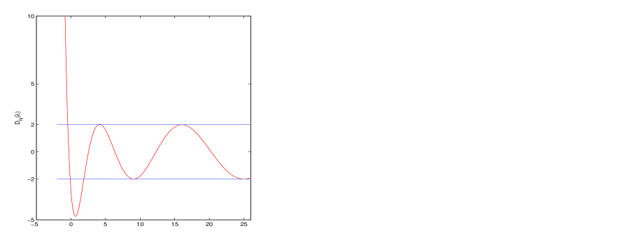
Figure 1: The polynomial $D_{N}(\lambda)$ for the Mathieu equation with the parameter $r=1$ calculated by means of formula (49) for $N=100$.

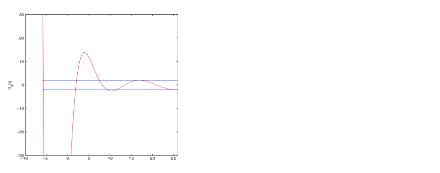
Figure 2: Same as in the previous figure but for $r=5$. The first minimum goes down to -292.0066.

As another example, consider the potential

$$V_{1}=\frac{\xi^{2}}{8}\left(1-\cos 4x\right)-3\xi\cos 2x~{},$$ (51)

which belongs to the quasi-exactly solvable family of the so-called trigonometric Razavy potentials [89]. The parameter $\xi$ is a positive real number. In Tables 4.3 and 4.4, the Razavy eigenvalues were calculated employing the SPPS  representation (39) for two different values of the parameter $\xi$. For comparison we use the eigenvalues given by Razavy analytically in terms of the parameter $\xi$ as follows [89]

$$\lambda_{0}=2\left(1-\sqrt{1+\xi^{2}}\right),\quad\lambda_{3}=4,\quad\lambda_{4}=2\left(1+\sqrt{1+\xi^{2}}\right)~{}.$$

Table 4.3: $\lambda_{n}$ for the Razavy Hamiltonian    $\xi=1$    $\xi=1$ $n$   $\lambda_{n}\ \text{(SPPS\thinspace)}$   $\lambda_{n}\ \text{(Ref. \cite[cite]{[\@@bibref{}{raz}{}{}]}\thinspace)}$ $0$ $-0.828430172936322$ $-0.828427124746190$ $1$ $-0.627099642286704$ $2$ $2.315154289053194$ $3$ $3.999948252396118$ $4$ $4$ $4.834668005757639$ $4.828427124746190$ $5$ $9.246360795065604$ $6$ $9.305957668676312$         

Table 4.4: $\lambda_{n}$ for the Razavy Hamiltonian    $\xi=2$    $\xi=2$ $n$   $\lambda_{n}\ \text{(SPPS\thinspace)}$   $\lambda_{n}\ \text{(Ref. \cite[cite]{[\@@bibref{}{raz}{}{}]})}\,$ $0$ $-2.472136690058546$ $-2.472135954999580$ $1$ $-2.428288532265432$ $2$ $3.193559545313260$ $3$ $4.000042398350143$ $4$ $4$ $6.472170127477180$ $6.472135954999580$ $5$ $9.864070609921770$ $6$ $10.253303565368553$   

In Figs. 3 and 4 we display the plots of the Hill discriminants for the values of the Razavy parameter $\xi=1$ and $\xi=2$, respectively. According to our results in subsection (4.6), the Hill discriminant is the same in the case of the supersymmetric partner potential

$$V_{2}=V_{1}+4\cos 2x\left(\frac{\xi}{2}-\frac{2A(\xi)}{\xi-A(\xi)\cos 2x}\right)+\frac{8A(\xi)\sin^{2}2x}{\left(\xi-A(\xi)\cos 2x\right)^{2}}$$ (52)

for the same values of the parameter $\xi$. In the latter equation $A(\xi)=\left(1-\sqrt{1+\xi^{2}}\right)$.

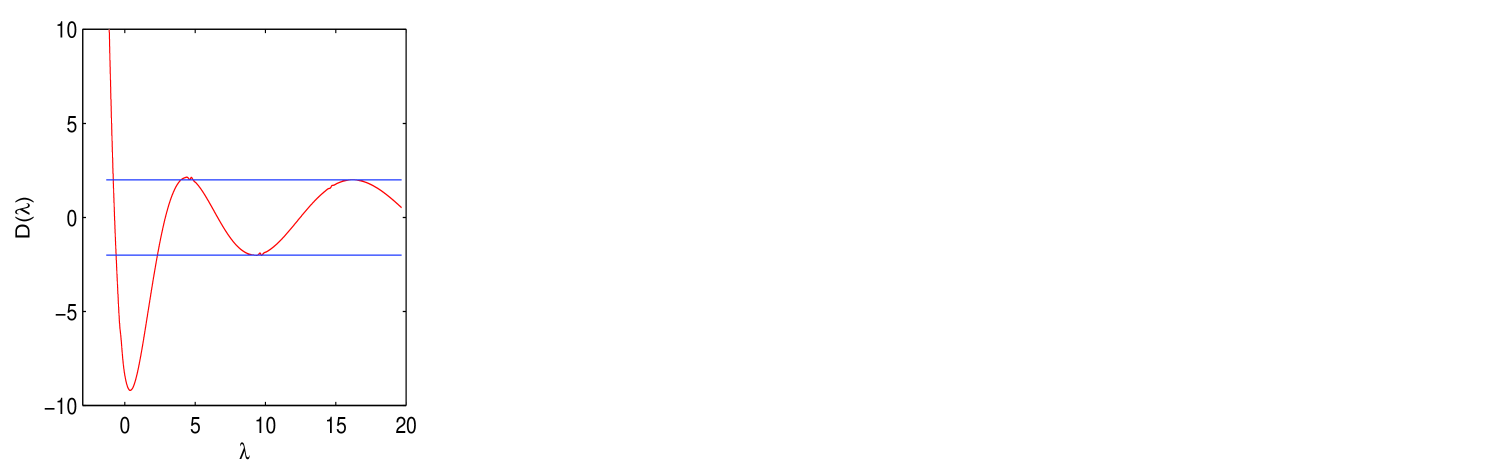
Figure 3: The polynomial $D_{N}(\lambda)$ for the Razavy equation with the parameter $\xi=1$ calculated by means of formula (49) for $N=100$.

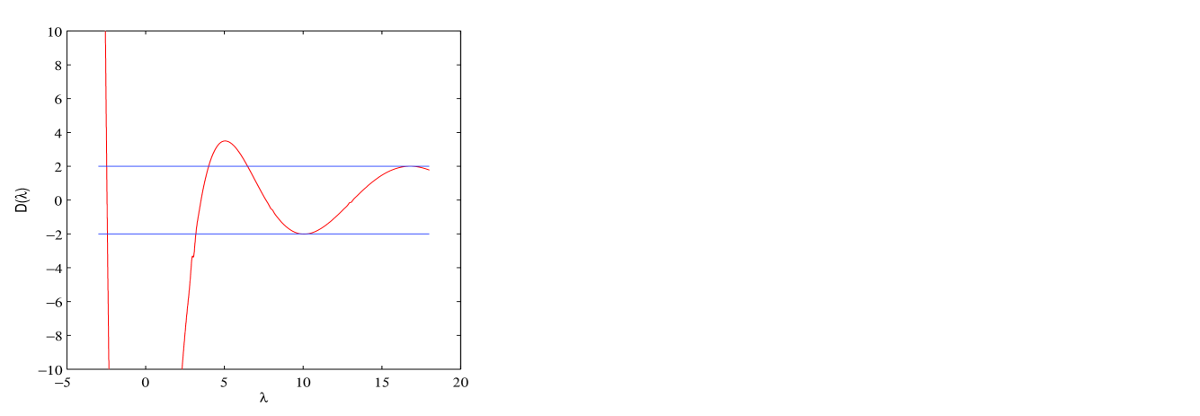
Figure 4: Same as in the previous figure but for $\xi=2$. The first minimum of Hill’s discriminant goes down to -55.01.

As final comments to this subsection, we believe that the calculation of the Hill discriminant through (49) offers clear numerical advantages with respect to other more complicated formulas for this important quantity provided in the literature, such as Jagerman’s so-called cardinal series representation [50], the infinite determinant representation involving the Fourier coefficients of the potential as well as the spectral parameter in the book of Magnus and Winkler [76], a matrix representation whose entries are complicated phase integrals obtained by the phase-integral method used by Fröman [40], and Boumenir’s representation in terms of integrals derived from the inverse spectral theory [9].

5 Spectral and transmission problems on the whole line

In this section we consider the one-dimensional Schrödinger equation

$$Hu(x)=-u^{\prime\prime}(x)+Q(x)u(x)=\lambda u(x),\quad x\in\mathbb{R},$$ (53)

where

$$Q(x)=\left\{\begin{array}[c]{cc}\alpha_{1},&x<0,\\ q(x),&0\leq x\leq h,\\ \alpha_{2},&x>h,\end{array}\right.$$ (54)

$\alpha_{1}$ and $\alpha_{2}$ are complex constants and $q$ is a continuous complex-valued function defined on the segment $[0,h]$. Thus, outside a finite segment the potential $Q$ admits constant values, and at the end points of the segment the potential may have discontinuities. We are interested in two classical problems. The first is the quantum-mechanical spectral problem, we are looking for such values of the spectral parameter $\lambda\in\mathbb{C}$ for which the Schrödinger equation possesses a solution $u$ belonging to the Sobolev space $H^{2}(\mathbb{R)}$ which in the case of the potential of the form (54) means that we are looking for solutions exponentially decreasing at $\pm\infty$.

The second consists in finding the reflectance and transmittance of the inhomogeneous layer described by $q$. We will formulate this problem in the form in which it arises in electromagnetic theory though both problems come not from one but from many different branches of physics and engineering.

5.1 Quantum-mechanical spectral problem

The eigenvalue problem (53) is one of the central in quantum mechanics for which $H$ is a self-adjoint operator in $L^{2}(\mathbb{R})$ with the domain $H^{2}(\mathbb{R)}.$ It implies that $Q$ is a real-valued function. In this case the operator $H$ has a continuous spectrum $[\min\left\{\alpha_{1},\alpha_{2}\right\},+\infty)$ and a discrete spectrum located on the set

$$[\min_{x\in[0,h]}q(x),\min\left\{\alpha_{1},\alpha_{2}\right\}).$$ (55)

Computation of energy levels of a quantum well described by the potential $Q$ is a problem of physics of semiconductor nanostructures (see, e.g., [44]). Other important models which reduce to the spectral problem (53) arise in studying the electromagnetic and acoustic wave propagation in inhomogeneous waveguides (see for instance [4], [21], [36], [22], [10], [85], [78]).

Hence in the applied problems it is important to have effective and rapid numerical methods for the solution of the problem (53). The most frequently applied is the shooting method (see, e.g., [44]). It has well known limitations due to the intrinsic difficulties of the shooting procedure, especially when the spectral parameter as in the problem under consideration participates in the boundary conditions (see equalities (57) and (60) below). It is much more convenient to have available an analytical form of a dispersion equation associated with the eigenvalue problem. In that case solutions of the dispersion equation can be approximated using different numerical techniques. However the dispersion equation is available only in really few examples (see [39]). There is another method developed for symmetric potentials [43]. Below we compare numerical results of our approach with the results from [43].

For simplicity we will assume that $\alpha_{1}$ and $\alpha_{2}$ are real constants and the function $q$ is a continuous real-valued function on $[0,h]$ though the presented method is applicable to the more general situation when $Q$ is complex valued. In this case necessary modifications must be made mainly in the reduction of the original problem on the whole line to a problem for the equation

$$-u^{\prime\prime}(x)+q(x)u(x)=\lambda u(x),\quad x\in(0,h)$$ (56)

with three boundary conditions at the end points of the interval $(0,h)$ (see below) meanwhile the application of the SPPS method suffers no essential changes. Our analysis follows that from [18].

For $x<0$ we have to consider the equation $-u^{\prime\prime}+(\alpha_{1}-\lambda)u=0$. Its solutions decreasing at $-\infty$ exist if only $\alpha_{1}-\lambda>0$. Denote $\mu=+\sqrt{\alpha_{1}-\lambda}$. Then the required solution for $x<0$ has the form $u(x)=c_{1}e^{\mu x}$ and the multiplicative constant can always be chosen equal to one. Thus, $u(x)=e^{\mu x}$, $x<0$, from where

$$u(0)=1\quad\text{and}\quad u^{\prime}(0)=\mu.$$ (57)

This gives us the initial conditions for the solution on the interval $(0,h)$ which we will construct following Theorem 1. For that we need first a nonvanishing particular solution of the equation

$$-u_{0}^{\prime\prime}(x)+q(x)u_{0}(x)=0$$ (58)

which as was explained in Section 2 can be constructed by means of the same SPPS method. Indeed, formulas (14)-(17) where $p$ should be chosen equal to $-1$ and $x_{0}=0$ give us a couple of linearly independent real-valued particular solutions $v_{1}$ and $v_{2}$ of (58). Hence (see Remark 4) the required nonvanishing solution of (58) can be chosen as $u_{0}=v_{1}+iv_{2}$. Let us notice that as $u_{0}(0)=1$ and $u_{0}^{\prime}(0)=i$ the initial conditions satisfied by the solutions of (56) $u_{1}$ and $u_{2}$ constructed according to (5) have the form

$$u_{1}(0)=u_{0}(0)=1,\quad u_{1}^{\prime}(0)=u_{0}^{\prime}(0)=i,$$

$$u_{2}(0)=0,\quad u_{2}^{\prime}(0)=-\frac{1}{u_{0}(0)}=-1.$$

From these relations we obtain that the solution of (56) satisfying the initial conditions (57) has the form

$$u(x)=u_{1}(x)+(i-\mu)u_{2}(x)\quad 0\leq x\leq h.$$ (59)

In the region $x>h$ the solution of equation (53) has the form

$$u(x)=C_{1}e^{-\sqrt{\alpha_{2}-\lambda}(x-h)}+C_{2}e^{\sqrt{\alpha_{2}-\lambda}(x-h)}$$

from which we obtain that the existence of an eigenfunction is possible if only $\sqrt{\alpha_{2}-\lambda}\in\mathbb{R}$. Hence $\alpha_{2}>\lambda$ and we denote $\nu=+\sqrt{\alpha_{2}-\lambda}$. Consequently, $u(x)=Ce^{-\nu(x-h)}$ and $u(h)=C$, $u^{\prime}(h)=-\nu C$ where $C$ is an arbitrary constant. Thus, the eigenvalues of the problem are such values of $\lambda$ for which the solution (59) satisfies the condition

$$u^{\prime}(h)+\nu u(h)=0$$ (60)

where, as above, $\nu=+\sqrt{\alpha_{2}-\lambda}$ and $\alpha_{2}>\lambda$.

In order to write down the explicit form of the dispersion equation (60) in terms of the spectral parameter power series we calculate the derivatives of the solutions of (56),

$$u_{1}^{\prime}=\frac{u_{0}^{\prime}}{u_{0}}u_{1}-\frac{\lambda}{u_{0}}{\displaystyle\sum\limits_{n=0}^{\infty}}\lambda^{n}\widetilde{X}^{(2n+1)}\quad\text{and}\quad u_{2}^{\prime}=\frac{u_{0}^{\prime}}{u_{0}}u_{2}-\frac{1}{u_{0}}{\displaystyle\sum\limits_{n=0}^{\infty}}\lambda^{n}X^{(2n)}.$$

Thus the derivative of the solution (59) has the form

$$u^{\prime}=\frac{u_{0}^{\prime}}{u_{0}}u-\frac{1}{u_{0}}\left({\displaystyle\sum\limits_{n=0}^{\infty}}\lambda^{n+1}\widetilde{X}^{(2n+1)}+(i-\mu){\displaystyle\sum\limits_{n=0}^{\infty}}\lambda^{n}X^{(2n)}\right).$$

Substituting this expression into (60) we arrive at the following result obtained in [18] and formulated here in the form of a theorem.

Theorem 7

Let $\alpha_{1}$, $\alpha_{2}$ be real numbers, $q$ be a real-valued continuous function defined on $[0,h]$ and $Q$ be defined by (54). Then $\lambda\in[\min_{x\in[0,h]}q(x),\min\left\{\alpha_{1},\alpha_{2}\right\})$ is an eigenvalue of the problem (53) if and only if the following dispersion equation

$$u_{0}^{\prime}(h)\left({\displaystyle\sum\limits_{n=0}^{\infty}}\lambda^{n}\widetilde{X}^{(2n)}(h)+\left(i-\sqrt{\alpha_{1}-\lambda}\right){\displaystyle\sum\limits_{n=0}^{\infty}}\lambda^{n}X^{(2n+1)}(h)\right)$$

$$-\frac{1}{u_{0}(h)}\left({\displaystyle\sum\limits_{n=0}^{\infty}}\lambda^{n+1}\widetilde{X}^{(2n+1)}(h)+\left(i-\sqrt{\alpha_{1}-\lambda}\right){\displaystyle\sum\limits_{n=0}^{\infty}}\lambda^{n}X^{(2n)}(h)\right)$$

$$+\sqrt{\alpha_{2}-\lambda}u_{0}(h)\left({\displaystyle\sum\limits_{n=0}^{\infty}}\lambda^{n}\widetilde{X}^{(2n)}(h)+\left(i-\sqrt{\alpha_{1}-\lambda}\right){\displaystyle\sum\limits_{n=0}^{\infty}}\lambda^{n}X^{(2n+1)}(h)\right)=0~{},$$ (61)

is satisfied and the corresponding (unique up to a multiplicative constant) eigenfunction has the form

$$u(x)=\left\{\begin{array}[c]{cc}e^{\mu x},&x<0,\\ u_{1}(x)+(i-\mu)u_{2}(x),&0\leq x\leq h,\\ \left(u_{1}(h)+(i-\mu)u_{2}(h)\right)e^{-\nu(x-h)},&x>h~{},\end{array}\right.$$

where $\mu=+\sqrt{\alpha_{1}-\lambda}$, $\nu=+\sqrt{\alpha_{2}-\lambda}$ and $u_{1}$, $u_{2}$ are defined by (5) where $u_{0}$ is the nonvanishing solution of (58) on $(0,h)$ satisfying the initial conditions $u_{0}(0)=1$ and $u_{0}^{\prime}(0)=i$, $p\equiv-1$, $r\equiv 1$ and $x_{0}=0$.

All the coefficients in equation (61): $u_{0}(h)$, $u_{0}^{\prime}(h)$, $\widetilde{X}^{(k)}(h)$ and $X^{(k)}(h)$ are easily and (as our numerical tests show) accurately obtained from the definitions introduced above, and the roots of the dispersion equation coincide with the eigenvalues of the problem and can be found using many available methods.

In what follows, let us consider a relatively simple situation: $\alpha_{1}=\alpha_{2}$. Rearranging the terms in equation (53) this case always can be reduced to the case $\alpha_{1}=\alpha_{2}=0$. Then $\nu=\mu=\sqrt{-\lambda}$, $\mu^{2}=-\lambda$ and $\lambda^{n}=(-1)^{n}\mu^{2n}$. The dispersion equation takes the form (here we correct some easily detectable misprints in [18])

$$u_{0}^{\prime}(h)\left(1+iX^{(1)}(h)\right)-\frac{i}{u_{0}(h)}$$

$$+{\displaystyle\sum\limits_{n=1}^{\infty}}(-1)^{n}\mu^{2n}(u_{0}^{\prime}(h)\widetilde{X}^{(2n)}(h)-\frac{1}{u_{0}(h)}\widetilde{X}^{(2n-1)}(h)+iu_{0}^{\prime}(h)X^{(2n+1)}(h)$$

$$-\frac{i}{u_{0}(h)}X^{(2n)}(h)+u_{0}(h)X^{(2n-1)}(h))$$

$$+{\displaystyle\sum\limits_{m=0}^{\infty}}(-1)^{m}\mu^{2m+1}(-u_{0}^{\prime}(h)X^{(2m+1)}(h)+\frac{1}{u_{0}(h)}X^{(2m)}(h)$$

$$+iu_{0}(h)X^{(2m+1)}(h)+u_{0}(h)\widetilde{X}^{(2m)}(h))=0.$$

Thus, the dispersion equation has the form

$$\sum_{k=0}^{\infty}a_{k}\mu^{k}=0$$ (62)

where

$$a_{0}=u_{0}^{\prime}(h)\left(1+iX^{(1)}(h)\right)-\frac{i}{u_{0}(h)},$$ (63)

$$a_{2n}=(-1)^{n}(u_{0}^{\prime}(h)\widetilde{X}^{(2n)}(h)-\frac{1}{u_{0}(h)}\widetilde{X}^{(2n-1)}(h)+iu_{0}^{\prime}(h)X^{(2n+1)}(h)$$

$$-\frac{i}{u_{0}(h)}X^{(2n)}(h)+u_{0}(h)X^{(2n-1)}(h)),\quad n\in\mathbb{N},$$ (64)

$$a_{2n+1}=(-1)^{n}(-u_{0}^{\prime}(h)X^{(2m+1)}(h)+\frac{1}{u_{0}(h)}X^{(2m)}(h)$$

$$+iu_{0}(h)X^{(2m+1)}(h)+u_{0}(h)\widetilde{X}^{(2m)}(h)),\quad n=0,1,2,\ldots.$$ (65)

The problem is reduced to the problem of finding zeros of an analytic function given by its Taylor series with the coefficients $a_{k}$, $k=0,1,2,\ldots$.

The usual approach to numerical solution of the considered eigenvalue problem consists in applying the shooting method (see, e.g., [44]) which is known to be unstable, relatively slow and to the difference of our approach does not offer any explicit equation for determining eigenvalues and eigenfunctions. In [43] another method based on approximation of the potential by square wells was proposed. It is limited to the case of symmetric potentials. The approach based on the SPPS is completely different and does not require any shooting procedure, approximation of the potential or numerical differentiation. Derived from the exact dispersion equation (62) we consider its approximation $\sum_{k=0}^{N}a_{k}\mu^{k}=0$ and in fact look for zeros of the polynomial $\sum_{k=0}^{N}a_{k}\mu^{k}$ in the interval $[\min q(x),0)$. Here we give only one example of numerical computation of eigenvalues referring to [18] for more examples and discussion.

We consider the potential $Q$ defined by the expression $Q(x)=-\upsilon\operatorname{sech}^{2}x$, $x\in(-\infty,\infty)$. It is not of a finite support, nevertheless its absolute value decreases rapidly when $x\rightarrow\pm\infty$. We approximate the original problem by a problem with a finite support potential $\widehat{Q}$ defined by the equality

$$\widehat{Q}(x)=\left\{\begin{array}[c]{cc}0,&x<-a\\ -\upsilon\operatorname{sech}^{2}x,&-a\leq x\leq a\\ 0,&x>a~{}.\end{array}\right.$$

An attractive feature of the potential $Q$ is that its eigenvalues can be calculated explicitly (see, e.g., [39]). In particular, for $\upsilon=m(m+1)$ the eigenvalue $\lambda_{n}$ is given by the formula $\lambda_{n}=-(m-n)^{2}$, $n=0,1,\ldots$.

The results of application of the SPPS method for $\upsilon=12$ are given in Table 5.1 in comparison with the exact values and the results from [43].

Table 5.1: Approximations of $\lambda_{n}$ of the Hamiltonian $H=-D^{2}-12\operatorname{sech}^{2}x$
$n$	Exact values	Numerical results from [43]	Numerical results using SPPS ($N=180$)
0	$-9$	$-9.094$	$-8.999628656$
1	$-4$	$-4.295$	$-3.999998053$
2	$-1$	$-0.885$	$-0.999927816$

5.2 Transmission problem for inhomogeneous layers

In this subsection we apply the SPPS method to the problem of finding the reflectance and transmittance of a finite inhomogeneous layer. This is a classical problem which still attracts a lot of attention due to its numerous applications in modern engineering, optical physics, solution of nonlinear problems and many other fields. Different methods for numerical solution of the problem have been proposed, mainly based on well known canonical techniques for approximate solution of ordinary differential equations such as the finite differences or expansion in power series (see, e.g., [56], [101], [54], [19]). One of the most used methods involves the approximation of the inhomogeneous layer by a structure consisting of many homogeneous layers (see, e.g., [60], [81], [27], [96]). Asymptotic methods such as the perturbation method or the WKB method are also applied to this problem (see, e.g., [42], [97], [82], [101]), though in the case of a finite inhomogeneous layer the WKB technique does not seem advantageous. Meanwhile the mentioned numerical approaches can give satisfactory results for certain fixed parameters of the problem their applicability is questionable when the solution of the problem is required, for example, for many different angles of incidence. The treatment of the oblique incidence case is not only interesting because of the many applications in which that incidence is needed - in optical filters, light couplers -, but also because sometimes the interfaces are rough - their effects and analysis depending on their size -, and/or are not parallel (see, e.g., [82]). This is due to imperfect deposition conditions. Such problems in the generation of the inhomogeneous layer (or multilayer) have generated systems in which the feedback of a reflectance, transmittance, or scattered light measurement is used to characterize the layer as it is created and to correct any discrepancies with the pre-established values. Such application must be able to recalculate the required correction profile and requires a real-time computation of transmittance and reflectance.

The mathematical statement of the problem involves a Helmholtz equation with a coefficient which is an arbitrary continuous function on a finite segment and constant outside. More precisely, the scalar function $u$ which represents a component of a linearly polarized electromagnetic wave in the case of an $s$-polarization satisfies the Helmholtz equation

$$u^{{}^{\prime\prime}}(x)+[k^{2}n^{2}(x)-\beta^{2}]u(x)=0$$ (66)

where $u$ stands for the transverse component of the electric field, and in the case of a $p$-polarization satisfies the following Sturm-Liouville equation (see, e.g., [49], [35])

$$n^{2}(x)\left(\frac{1}{n^{2}(x)}v^{\prime}(x)\right)^{\prime}+[k^{2}n^{2}(x)-\beta^{2}]v(x)=0$$ (67)

in which $v$ represents the transverse component of the magnetic field. Here $k$ is the free-space circular wave number. The refractive index $n$ preserves constant values $n_{1}$ and $n_{2}$ in the regions $x<0$ and $x>d$ respectively and is an arbitrary continuous function in the interval $0\leq x\leq d$ (see figure 5). For simplicity we assume $n$ to be real valued though the method is equally applicable to the case of a complex refractive index.

The propagation constant $\beta$ is related to the angle of incidence of the wave in the following way $\beta=k\sin\theta$ (see, e.g., [49]), and $\beta$ vanishes in the case of normal incidence.

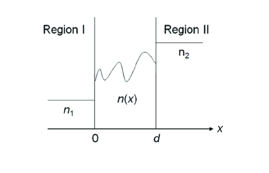
Figure 5: An inhomogeneous layer.

In spite of the fact that equations (66) and (67) describe the behaviour of different components of an electromagnetic wave, corresponding to an electric and a magnetic field respectively, there exists a simple transformation from (67) to (66) and vice versa (see, e.g., [49]). Namely, if $v$ is a solution of (67) then $U=v/n$ is a solution of the equation

$$U^{{}^{\prime\prime}}(x)+[k^{2}N^{2}(x)-\beta^{2}]U(x)=0$$

where $k^{2}N^{2}=k^{2}n^{2}+n^{{}^{\prime\prime}}/n-2\left(n^{\prime}/n\right)^{2}$. Thus, in both cases the problem reduces to an equation of the form (66).

We denote $k_{1}=\sqrt{k^{2}n_{1}^{2}-\beta^{2}}$ and $k_{2}=\sqrt{k^{2}n_{2}^{2}-\beta^{2}}$. The solution $u$ of (66) or $v$ of (67) respectively together with their first derivatives must be continuous at all $x$ including the points $x=0$ and $x=d$. The incident wave in the region I (see figure 6)

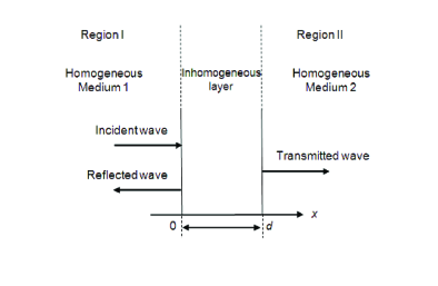
Figure 6: Incident, reflected and transmitted waves.

is assumed to have the form $e^{-ik_{1}x},$ and together with the reflected wave the whole solution for $x<0$ is the combination

$$u(x)=e^{-ik_{1}x}+Re^{ik_{1}x},\quad x<0$$

where the constant $R$ is the reflection coefficient whose absolute value is less than 1. The solution corresponding to the transmitted wave in the region II has the form

$$u(x)=Te^{-ik_{2}x},\quad x>d$$

where $T$ is the transmission coefficient. In the case of unabsorbent media for the normally incident waves the following energy conservation relation holds

$$\left|R\right|^{2}+n_{2}\left|T\right|^{2}/n_{1}=1.$$ (68)

Let us suppose that the two linearly independent solutions $y_{1}$ and $y_{2}$ of (66) in the interval of inhomogenicity $0\leq x\leq d$ are known such that the following initial conditions are satisfied:

$$y_{1}(0)=1,\quad y_{1}^{\prime}(0)=0$$ (69)

and

$$y_{2}(0)=0,\quad y_{2}^{\prime}(0)=1.$$ (70)

Then we are able to obtain analytic expressions for $R$ and $T$  in terms of $u_{1}$ and $u_{2}$ [17]. We have

$$R=\frac{-k_{1}k_{2}y_{2}(d)-y_{1}^{\prime}(d)-ik_{2}y_{1}(d)+ik_{1}y_{2}^{\prime}(d)}{[y_{1}^{\prime}(d)-k_{1}k_{2}y_{2}(d)]+i[k_{2}y_{1}(d)+k_{1}y_{2}^{\prime}(d\text{ })]}$$ (71)

and

$$T=\frac{2ik_{1}[y_{1}(d)y_{2}^{\prime}(d)-y_{1}^{\prime}(d)y_{2}(d)]e^{ik_{2}d}}{[y_{1}^{\prime}(d)-k_{1}k_{2}y_{2}(d)]+i[k_{2}y_{1}(d)+k_{1}y_{2}^{\prime}(d)]}.$$ (72)

These formulas remain valid for equation (67) when one substitutes $y_{1}$ and $y_{2}$ with the solutions $v_{1}$ and $v_{2}$ of (67) satisfying the initial conditions (69) and (70) respectively).

Thus, the transmission problem for an inhomogeneous layer consists in computing a couple of solutions of (66) (or (67)) in the interval of inhomogenicity $0\leq x\leq d$, satisfying the initial conditions (69) and (70), and then the reflection and transmission coefficients are found from (71) and (72). For computation of these solutions we use theorem 1 and take into account (11) and (12) where it is convenient to choose $x_{0}=0$.

There are several examples of explicitly solvable inhomogeneous profiles [80], [101]. These were used in [17] for testing the results obtained by means of SPPS. In all numerical simulations the achieved accuracy was remarkable.

6 Zakharov-Shabat eigenvalue problem

In this section we study the Zakharov-Shabat system with a real-valued potential. It arises in the solution via the inverse scattering method of several nonlinear evolution equations such as the nonlinear Schrödinger equation, the sine-Gordon equation and the modified Korteweg-de Vries equation. For example, in the case of the nonlinear Schrödinger equation, eigenvalues of the Zakharov-Shabat system correspond to soliton solutions implemented in fiber optics (see, e.g., [45]). The assumption that the potential is real valued is natural and common in the engineering literature,- it includes the conventional profiles such as the rectangular, the Gaussian and the hyperbolic secant.

In [68] a general solution of the Zakharov-Shabat system with a real potential in terms of SPPS was obtained and used for deriving a dispersion equation corresponding to the eigenvalue problem with a compactly supported potential. Once again the problem is reduced to a problem of localizing zeros of an analytic function given by its Taylor series. For numerical approximation of eigenvalues one can consider a truncated series and thus for practical computation the eigenvalue problem reduces to finding roots of a polynomial.

The Zakharov-Shabat system with a real potential has the form [102], [70]

$$\partial n_{1}(x)-\lambda n_{1}(x) =U(x)n_{2}(x)$$ (73)

$$\partial n_{2}(x)+\lambda n_{2}(x) =-U(x)n_{1}(x)~{},$$ (74)

where $\partial:=\frac{d}{dx}$; $U:\mathbb{R}\rightarrow\mathbb{R}$ is the potential and $U\in L_{1}(-\infty,\infty)$; the solutions $n_{1}$ and $n_{2}$ in general are complex valued and the spectral parameter $\lambda$ is a complex constant. It is convenient to rewrite the Zakharov-Shabat system using the following notations

$$u=n_{1}+in_{2},\qquad v=n_{1}-in_{2},\qquad q=iU~{}.$$

Then (73), (74) takes the form of a Dirac system with a scalar potential (see, e.g., [15], [47], [48], [84])

$$(\partial+q(x))u=\lambda v,$$ (75)

$$(\partial-q(x))v=\lambda u~{}.$$ (76)

From these equalities it is easy to see that $u$ and $v$ are solutions of the following second-order differential equations

$$(\partial-q(x))(\partial+q(x))u(x)=\lambda^{2}u(x)$$ (77)

and

$$(\partial+q(x))(\partial-q(x))v(x)=\lambda^{2}v(x)~{}.$$ (78)

The differential operators on the left-hand side can be written in the form of stationary Schrödinger operators describing supersymmetric partners

$$(\partial-q)(\partial+q)=\partial^{2}+(\partial q-q^{2})\quad\text{and}\quad(\partial+q)(\partial-q)=\partial^{2}-(\partial q+q^{2}).$$

Nevertheless, precisely the factorized form (77), (78) presents certain advantage for applying the SPPS method due to the possibility to write down closed-form solutions of (77) and (78) for $\lambda=0$. Namely, let $Q(x)=\int q(x)dx$. Then $u_{0}(x)=e^{-Q(x)}$ and $v_{0}(x)=e^{Q(x)}$ are solutions of the equations $(\partial-q)(\partial+q)u_{0}=0$ and $(\partial+q)(\partial-q)v_{0}=0$ respectively. Note that for a continuous function $q$ defined on a closed finite interval both $u_{0}$ and $v_{0}$ are devoid of zeros.

The systems of auxiliary functions $\left\{X^{(n)}\right\}_{n=0}^{\infty}$ and $\left\{\widetilde{X}^{(n)}\right\}_{n=0}^{\infty}$ in this case are defined as follows

$$X^{(0)}(x)\equiv\tilde{X}^{(0)}(x)\equiv 1,$$ (79)

$$X^{(n)}(x)=\int_{x_{0}}^{x}X^{(n-1)}(s)e^{(-1)^{n}2Q(s)}ds,$$ (80)

$$\tilde{X}^{(n)}(x)=\int\limits_{x_{0}}^{x}\tilde{X}^{(n-1)}(s)e^{(-1)^{n+1}2Q(s)}ds.$$ (81)

We obtain the following SPPS form of a general solution of the Zakharov-Shabat system.

Theorem 8

[68] Let $U$ be a continuous real-valued function defined on a finite segment $[a,b]\subset\mathbb{R}$. Then the general solution of the Zakharov-Shabat system (73), (74) has the form

$$n_{1}(x)=\dfrac{c_{1}}{2}\sum_{n=0}^{\infty}e^{(-1)^{n}Q(x)}\lambda^{n}\tilde{X}^{(n)}(x)+\dfrac{c_{2}}{2\lambda}\sum_{n=0}^{\infty}e^{(-1)^{n+1}Q(x)}\lambda^{n}X^{(n)}(x),$$ (82)

$$n_{2}(x)=\dfrac{ic_{1}}{2}\sum_{n=0}^{\infty}(-1)^{n}e^{(-1)^{n}Q(x)}\lambda^{n}\tilde{X}^{(n)}(x)-\dfrac{ic_{2}}{2\lambda}\sum_{n=0}^{\infty}(-1)^{n}e^{(-1)^{n+1}Q(x)}\lambda^{n}X^{(n)}(x),$$ (83)

where $c_{1}$ and $c_{2}$ are arbitrary complex constants, $Q$ is an antiderivative of $q=iU$, $x_{0}\in[a,b]$ and the series converge uniformly in $[a,b]$.

Solutions of the Zakharov-Shabat system (73), (74) satisfying the following asymptotic relations

$$\vec{\sigma}(x,\lambda) \cong\binom{1}{0}e^{\lambda x}\text{,\quad\ }x\rightarrow-\infty,$$ (84)

$$\vec{\xi}(x,\lambda) \cong\binom{0}{1}e^{-\lambda x}\text{,\quad}x\rightarrow\infty$$ (85)

are called the Jost solutions [1]. The eigenvalue problem for the Zakharov-Shabat system with a real valued potential consists in finding such values of the spectral parameter $\lambda$ for which $\operatorname*{Re}\lambda>0$ and there exists a nontrivial solution $\vec{n}$ satisfying the Jost conditions (84) and (85).

If the real valued potential $U$ has a compact support on the segment $[-a,a]$ it is easy to see that the eigenvalue problem reduces to find such values of $\lambda$ ($\operatorname*{Re}\lambda>0$) for which there exists a solution of (73), (74) satisfying the following boundary conditions

$$n_{1}(-a)=1, \hskip 28.45274ptn_{2}(-a)=0,$$ (86)

$$n_{1}(a)=0.$$ (87)

We refer here to [58] and [59] for estimates of the number of real eigenvalues of a compactly supported potential.

The next statement gives us a dispersion equation equivalent to the Zakharov-Shabat eigenvalue problem for the real, compactly supported potentials.

Theorem 9

[68] Let $U$ be a continuous real-valued function with a compact support on the segment $[-a,a]$. Then $\lambda$ ($\operatorname*{Re}\lambda>0$) is an eigenvalue of the Zakharov-Shabat system if and only if the following equation is satisfied

$$\sum\limits_{n=0}^{\infty}\lambda^{n}\left(e^{(-1)^{n}Q(a)}\tilde{X}^{(n)}(a)+e^{(-1)^{n+1}Q(a)}X^{(n)}(a)\right)=0~{},$$ (88)

where $Q(x)=i\int\limits_{-a}^{x}U(t)dt$ and $x_{0}=-a$ in (6)-(7).

If $\lambda$ is an eigenvalue then the corresponding eigenvector is given by

$$\overrightarrow{n}=\vec{\psi}+\vec{\varphi}$$

with

$$\vec{\psi}(x)=\binom{\psi_{1}(x)}{\psi_{2}(x)}= \left(\begin{array}[c]{c}\dfrac{1}{2}\sum\limits_{n=0}^{\infty}e^{(-1)^{n}Q(x)}\lambda^{n}\tilde{X}^{(n)}(x)\\ \dfrac{i}{2}\sum\limits_{n=0}^{\infty}(-1)^{n}e^{(-1)^{n}Q(x)}\lambda^{n}\tilde{X}^{(n)}(x)\end{array}\right),$$ (91)

$$\vec{\varphi}(x)=\binom{\varphi_{1}(x)}{\varphi_{2}(x)}= \left(\begin{array}[c]{c}\dfrac{1}{2}\sum\limits_{n=0}^{\infty}e^{(-1)^{n+1}Q(x)}\lambda^{n}X^{(n)}(x)\\ -\dfrac{i}{2}\sum\limits_{n=0}^{\infty}(-1)^{n}e^{(-1)^{n+1}Q(x)}\lambda^{n}X^{(n)}(x)\end{array}\right).$$ (94)

The theorem reduces the Zakharov-Shabat eigenvalue problem with a compactly supported potential to the problem of localizing zeros (in the right half-plane) of an analytic function $\kappa(\lambda)=\sum\limits_{n=0}^{\infty}a_{n}\lambda^{n}$ of the complex variable $\lambda$ with the Taylor coefficients $a_{n}$ given by the expressions

$$a_{n}=e^{(-1)^{n}Q(a)}\tilde{X}^{(n)}(a)+e^{(-1)^{n+1}Q(a)}X^{(n)}(a).$$ (95)

Equation (88) represents a dispersion equation of the eigenvalue problem. The coefficients $a_{n}$ can be easily and accurately calculated following the definitions introduced above. For the numerical solution of the eigenvalue problem one can consider a polynomial

$$\kappa_{N}(\lambda)=\sum\limits_{n=0}^{N}a_{n}\lambda^{n}$$ (96)

approximating the function $\kappa$. For a reasonably large $N$ its roots give an accurate approximation of the eigenvalues of the problem.

As a numerical example we consider the rectangular box referring the reader to [68] for further numerical tests and details. For the rectangular box the exact solution satisfying the boundary conditions (86)  is known. Such system can be applied to describe the problem of the diffraction of a wave by a screen with a slit (see [75]). Discrete eigenvalues of the spectral parameter can also be approximated using a variational principle approach [52]. The potential is defined by the equality

$$U(x)=\left\{\begin{array}[c]{ll}A,&\left|x\right|<a,\\ 0,&\text{elsewhere.}\end{array}\right.$$

A dispersion equation in this case can be obtained explicitly and written as follows

$$\gamma\cos 2\gamma+\lambda\sin 2\gamma=0~{},$$ (97)

where $\gamma=\sqrt{A^{2}-\lambda^{2}}$.

For solving the dispersion equation (97) the routine NSolve of Wolfram Mathematica 7 was used. We considered $a=1$. In the case $A=1$ the routine NSolve delivers one solution of (97) $\lambda_{0}^{NSolve}=0.31902252414261895$. Application of the SPPS method with $m=2000$ and $N=120$ gives us the value $\lambda_{0}=0.31902252414254$. The agreement is up to the 12th digit. Taking $m=4000$ and $N=180$ we obtain still a better approximation $\lambda_{0}=0.319022524142619$. The agreement is up to the 14th digit.

In the case $A=4$ there are three eigenvalues. NSolve delivers the following values $\lambda_{0}^{NSolve}=0.41262411401896715$, $\lambda_{1}^{NSolve}=2.8945478628320327$ and $\lambda_{2}^{NSolve}=3.749624961605374$. Application of the SPPS method with $m=2000$ and $N=100$ gives us the values $\lambda_{0}=0.412624114002$, $\lambda_{1}=2.8945478628329$ and $\lambda_{2}=3.7496249616095$, and with $m=4000$ and $N=180$: $\lambda_{0}=0.4126241140179$, $\lambda_{1}=2.89454786283226$ and $\lambda_{2}=3.7496249616045$.

7 Conclusions

We presented a review of recent research and applications of spectral parameter powers series (SPPS) representations for solving initial and boundary value problems as well as spectral and related problems for Sturm-Liouville equations. Application of the SPPS approach allows one to obtain explicit analytic forms of characteristic equations for a variety of problems. Approximation of these equations represents a powerful, universal and accurate numerical method highly competitive with the best purely computational techniques. The SPPS method is algorithmically simple and can be easily implemented using available routines of such environments for scientific computing as Matlab.

Acknowledgments

This research was partially supported by CONACYT, Mexico via the research project 50424.

References

- [1] M.J. Ablowitz and H. Segur, Solitons and the inverse scattering transform (SIAM, Philadelphia, 1981).
- [2] R.P. Agarwal, Difference equations and Inequalities (Marcel Dekker, New York, 1992).
- [3] R. Ashino, M. Nagase and R. Vaillancourt, Behind and beyond the Matlab ODE suite, Computers and Mathematics with Applications 40 (2000) 491-512.
- [4] C.A. Balanis, Advanced Engineering Electromagnetics (John Wiley & Sons, New York, 1989)
- [5] H. Begehr and R. Gilbert, Transformations, transmutations and kernel functions, vol. 1–2 (Harlow: Longman Scientific & Technical, 1992).
- [6] R. Bellman, Perturbation techniques in mathematics, engineering and physics (Dover Publications, New York, 2003).
- [7] J. Ben Amara and A.A. Shkalikov, A Sturm-Liouville problem with physical and spectral parameters in boundary conditions, Math. Notes 66 (1999) 127–134.
- [8] F. Bloch, Ueber die Quantenmechanik der Elektronen in Kristallgittern, Z. Physik 52 (1928) 555–600.
- [9] A. Boumenir, Eigenvalues of periodic Sturm-Louville problems by the Shannon-Whittaker sampling theorem, Math. Comp. 68 (1999) 1057-1066.
- [10] L.M. Brekhovskikh, Waves in layered media (Academic Press, New York, 1960).
- [11] H. Campos and V.V. Kravchenko, A finite-sum representation for solutions for the Jacobi operator, Journal of Difference Equations and Applications 17 (2011) 567–575.
- [12] H. Campos, V.V. Kravchenko and L. Mendez, Complete families of solutions for the Dirac equation: an application of bicomplex pseudoanalytic function theory and transmutation operators, Submitted to Advances in the Applied Clifford Algebras (available from arXiv.org., 2011).
- [13] H. Campos, V.V. Kravchenko and S. Torba, Transmutations, L-bases and complete families of solutions of the stationary Schrödinger equation in the plane, Journal of Mathematical Analysis and Applications, 389 (2012) 1222-1238.
- [14] R.W. Carroll, Transmutation theory and applications Mathematics Studies 117 ( North-Holland, Amsterdam, 1985).
- [15] J. Casahorrán, Solving simultaneously Dirac and Riccati equations, J. Nonlin. Math. Phys. 5 (1998) 371-382.
- [16] K.M. Case, Singular potentials, Phys. Rev. 80 (1950) 797–806.
- [17] R. Castillo, K.V. Khmelnytskaya, V.V. Kravchenko and H. Oviedo, Efficient calculation of the reflectance and transmittance of finite inhomogeneous layers, J. Opt. A: Pure and Applied Optics 11 (2009) 065707.
- [18] R. Castillo, V.V. Kravchenko, H. Oviedo and V.S. Rabinovich, Dispersion equation and eigenvalues for quantum wells using spectral parameter power series, J. Math. Phys. 52 (2011) 043522.
- [19] M. Chamanzar, K. Mehrany and B. Rashidian, Legendre polynomial expansion for analysis of linear one-dimensional inhomogeneous optical structures and photonic crystals, J. Opt. Soc. Am. B 2 (2006) 969-977.
- [20] B. Chanane, Sturm-Liouville problems with parameter dependent potential and boundary conditions, J. Comput. Appl. Math. 212 (2008) 282–290.
- [21] A.H. Cherin, An introduction to Optical Fibers (McGraw-Hill, 1983).
- [22] W.C. Chew, Waves and fields in inhomogeneous media (Van Nostrand Reinhold, New York, 1990).
- [23] W.J. Code and P.J. Browne, Sturm-Liouville problems with boundary conditions depending quadratically on the eigenparameter, J. Math. Anal. Appl. 309 (2005) 729–742.
- [24] F. Cooper, A. Khare, and U. Sukhatme, Supersymmetry in quantum mechanics (World Scientific, Singapore, 2001).
- [25] F. Correa,V. Jakubský and M.S. Plyushchay, Finite-gap systems, tri-supersymmetry and self-isospectrality, J. Phys. A: Math. Gen. 41 (2008) 485303.
- [26] H. Coşkun and N. Bayram, Asymptotics of eigenvalues for regular Sturm-Liouville problems with eigenvalue parameter in the boundary condition, J. Math. Anal. Appl. 306 (2005) 548–566.
- [27] L. De Caro and M.C. Ferrara, Simple method for the determination of optical parameters of inhomogeneous thin films, Thin Solid Films 342 (1999) 153-159.
- [28] J. Delsarte and J.L. Lions, Transmutations d’opérateurs différentiels dans le domaine complexe, Comment. Math. Helv. 32 (1956) 113-128.
- [29] M. Desaix, D. Anderson and M. Lisak, Eigenvalues of the Zakharov-Shabat scattering problem for two separated sech-shaped pulses, Phys. Lett. A 372 (2008) 2386-2390.
- [30] M. Desaix, D. Anderson, M. Lisak and M.L. Quiroga-Teixeiro, Variationally obtained approximate eigenvalues of the Zakharov-Shabat scattering problem for real potentials, Phys. Lett. A 212 (1996) 332-338.
- [31] C. Desem and P.L. Chu, Soliton-Soliton interaction, in Optical solitons - theory and experiment, ed. J.R. Taylor (Cambridge Univ. Press, Cambridge, 1992).
- [32] J.A. Dobrowolski and P.G. Verly, Inhomogeneous and Quasi-Inhomogeneous Optical Coatings (Proc. SPIE 2046, 1993).
- [33] M.S.P. Eastham, The Spectral Theory of Periodic Differential Equations (Scottish Academic Press, Edinburgh and London, 1973).
- [34] M.K. Fage and N.I. Nagnibida, The problem of equivalence of ordinary linear differential operators, (Nauka, Novosibirsk, 1987).
- [35] D. Felbacq and F. Zolla, Scattering theory of photonic crystals, in Introduction to complex mediums for optics and electromagnetics, eds. W. S. Weiglhofer and A. Lakhtakia (SPIE Press, 2003) 365-393.
- [36] L.B. Felsen and N. Marcuvitz, Radiation and Scattering of Waves, (IEEE Press, New York, 1994).
- [37] C.D.J. Fernández, B. Mielnik, O. Rosas-Ortiz and B.F. Samsonov, Nonlocal supersymmetric deformations of periodic potentials, J. Phys. A: Math Gen. 35 (2002) 4279-4291.
- [38] G. Floquet, Sur les equations differentialles lineaires a coefficients périodiques, Ann. Ecole Norm. Sup. 12 (1883) 47-88.
- [39] S. Flügge, Practical Quantum Mechanics (Springer-Verlag, Berlin, 1994).
- [40] N. Fröman, Dispersion relation for energy bands and energy gaps derived by the use of a phase-integral method with an application to the Mathieu equation, J. Phys. A: Math Gen. 12 (1979) 2355-2372.
- [41] Ch. T. Fulton, Two-point boundary value problems with eigenvalue parameter contained in the boundary conditions, Proc. Roy. Soc. Edinburgh A 77 (1977) 293–308.
- [42] J.F. Hall Jr., Reflection coefficient of optically inhomogeneous layers, J. Opt. Soc. Am. 48 (1958) 654-657.
- [43] R.L. Hall, Square-well representations for potentials in quantum mechanics, J. Math. Phys. 33 (1992) 3472-3476.
- [44] P. Harrison, Quantum Wells, Wires and Dots: Theoretical and Computational Physics of Semiconductor Nanostructures (Wiley, Chichester, 2010).
- [45] A. Hasegawa and Y. Kodama, Solitons in optical communications (Clarendon, Oxford, 1995).
- [46] G.W. Hill, On the part of the motion of lunar perigee which is a function of the mean motions of the sun and moon, Acta Math. 8 (1886) 1–36.
- [47] J.R. Hiller, Solution of the one-dimensional Dirac equation with a linear scalar potential, Am. J. Phys. 70 (2002) 522-524.
- [48] C.-L. Ho, Quasi-exact solvability of Dirac equation with Lorentz scalar potential, Ann. Phys. 321 (2006) 2170-2182.
- [49] A. Ishimaru, Electromagnetic wave propagation, radiation, and scattering (Prentice Hall, New Jersey, 1991).
- [50] D.L. Jagerman, The discriminant of Hill’s equation, (Research Report No. BR-39, New York University, Courant Inst. Math. Sci., 1962).
- [51] H.M. James, Energy bands and wave functions in periodic potentials, Phys. Rev. 76 (1949) 1602-1610.
- [52] D.J. Kaup and B.A. Malomed, Variational principle for the Zakharov-Shabat equations, Physica D 84 (1995) 319-328.
- [53] W.G. Kelley and A.C. Peterson, The Theory of Differential Equations: Classical and Qualitative (Springer, Berlin, 2010).
- [54] M. Khalaj-Amirhosseini, Analysis of lossy inhomogeneous planar layers using Taylor’s series expansion, IEEE Trans. Antennas and Propag. 54 (2006) 130-135.
- [55] K.V. Khmelnytskaya and H.C. Rosu, A new series representation for Hill’s discriminant, Ann. Phys. 325 (2010) 2512-2521.
- [56] M. Kildemo, O. Hunderi and B. Drévillon, Approximation of reflection coefficients for rapid real-time calculation of inhomogeneous films, J. Opt. Soc. Am. A 14 (1997) 931-939.
- [57] A.C. King, J. Billingham and S.R. Otto, Differential equations (Cambridge University Press, Cambridge, 2003).
- [58] M. Klaus and J.K. Shaw, Purely imaginary eigenvalues of Zakharov-Shabat systems, Phys. Rev. E 65 (2002) 036607.
- [59] M. Klaus and J.K. Shaw, On the eigenvalues of Zakharov-Shabat systems, SIAM J. Math Anal. 34 (2003) 759-773.
- [60] Z. Knittl, A method of integration for the inhomogeneous layer, Czech. J. Phys. B 18 (1968) 763-770.
- [61] A. Kostenko and G. Teschl, On the singular Weyl–Titchmarsh function of perturbed spherical Schrödinger operators, J. Differential Equations 250 (2011) 3701–3739.
- [62] V.V. Kravchenko, A representation for solutions of the Sturm-Liouville equation, Complex Variables and Elliptic Equations 53 (2008) 775-789.
- [63] V.V. Kravchenko, Applied Pseudoanalytic Function Theory (Birkhäuser, Basel, Series: Frontiers in Mathematics, 2009).
- [64] V.V. Kravchenko, On the completeness of systems of recursive integrals, Communications in Mathematical Analysis Conf. 03 (2011) 172–176.
- [65] V.V. Kravchenko, S. Morelos and S. Tremblay, Complete systems of recursive integrals and Taylor series for solutions of Sturm-Liouville equations, To appear in Mathematical Methods in the Applied Sciences (2012).
- [66] V.V. Kravchenko, R.M. Porter, Spectral parameter power series for Sturm-Liouville problems, Mathematical Methods in the Applied Sciences 33 (2010) 459-468.
- [67] V.V. Kravchenko and S.M. Torba, Transmutations for Darboux transformed operators with applications, J Phys A: Math. and Theor. 45 (2012) 075201.
- [68] V.V. Kravchenko and U. Velasco-García, Dispersion equation and eigenvalues for the Zakharov-Shabat system using spectral parameter power series, J. Math. Phys. 52 (2011) 063517.
- [69] R. de L. Kronig and W.G. Penney, Quantum mechanics of electrons in crystal lattices, Proc. Roy. Soc. (London) A 130 (1931) 499–513.
- [70] G.L. Lamb, Elements of soliton theory (John Wiley and Sons, New York, 1980).
- [71] B.M. Levitan, Inverse Sturm-Liouville problems (VSP, Zeist., 1987).
- [72] B.M. Levitan and I.S. Sargsjan, Sturm-Liouville and Dirac operators (Kluwer Acad. Publ., Dordrecht, 1991)
- [73] A. Liapounoff, Sur une série dans la théorie des équations difféntielles du second ordre á coefficients periodiques, Mem. Acad. Imp. Sci. St. Petersbourg(= Akad. Nauk Zapiski) (8) XIII (1902) (Union List of Serials, 3rd ed., Vol. 1, p. 113).
- [74] K.-J. Liu, L. He, G.-L. Zhou and Y.-J. Wu, New exactly solvable supersymmetric periodic potentials, Chin. Phys. 10 (2001) 1110-1112.
- [75] S.V. Manakov, Nonlinear Fraunhofer diffraction, Sov. Phys. JETP 38 (1974) 693-696.
- [76] W. Magnus and S. Winkler, Hill’s Equation (Interscience, New York, 1966).
- [77] V.A. Marchenko, Sturm-Liouville operators and applications (Birkhäuser, Basel, 1986).
- [78] H. Medwin and C.S. Clay, Fundamentals of Oceanic Acoustics (Academic Press, Boston, San Diego, New York, 1997).
- [79] E.V. Moiseenko and A.B. Shvartsburg, Broadband nonreflecting properties of thin inhomogeneous coatings for arbitrarily polarized electromagnetic waves in a wide range of angles of incidence, Opt. and Spectroscopy 95, 771-776.
- [80] S. Monaco, Reflectance of an inhomogeneous thin film, J. Opt. Soc. Am. 51 (1961) 280-282.
- [81] M. Montecchi, Characterization of inhomogeneous optical interference films using a complex parabolic profile model, Pure Appl. Opt. 4 (1995) 831-839.
- [82] M. Montecchi, R.M. Montereali and E. Nichelatti, Reflectance and transmittance of a slightly inhomogeneous thin film bounded by rough, unparallel interfaces, Thin Solid Films 396 (2001) 262-273.
- [83] National Bureau of Standards, Tables relating to Mathieu functions (Columbia University Press, New York, 1951).
- [84] Y. Nogami and F.M. Toyama, Supersymmetry aspects of the Dirac equation in one dimension with a Lorentz scalar potential, Phys. Rev. A 47 (1993) 1708-1714.
- [85] O.A. Obrezanova and V.S. Rabinovich, Acoustic field, generated by moving source in stratified waveguides, Wave Motion 27 (1998) 155-167.
- [86] Y. Pinchover and J. Rubinstein, An introduction to partial differential equations (Cambridge University Press, Cambridge, 2005).
- [87] A.R. Plastino, A. Rigo, M. Casas, F. Garcias and A Plastino, Supersymmetric approach to quantum systems with position-dependent effective mass, Phys. Rev. A 60 (1999) 4318-4325.
- [88] J. Pöschel and E. Trubowitz, Inverse spectral theory (Academic Press, New York, 1987).
- [89] M. Razavy, A potential model for torsional vibrations of molecules, Phys. Lett. A 82 (1981) 7–9.
- [90] J. Satsuma and N. Yajima, Initial value problems of one-dimensional self-modulation of nonlinear waves in dispersive media, Prog. Theor. Phys. Suppl. 55 (1974) 284-306.
- [91] F.L. Scarf, New soluble energy band problem, Phys. Rev. 112 (1958) 1137-1140.
- [92] L. Shampine and M. Reichelt, The Matlab ODE suite, SIAM J. Sci. Comput. 18 (1997) 1-22.
- [93] A.B. Shvartsburg, G. Petite and P. Hecquet, Broadband antireflection properties of thin heterogeneous dielectric films, J. Opt. Soc. Am. A 17 (2000) 2267-2271.
- [94] J.C. Slater, A soluble problem in energy bands. Phys. Rev. 87 (1952) 807–835.
- [95] A. Stanoyevitch, Introduction to Numerical Ordinary and Partial Differential Equations Using Matlab (Wiley-Interscience, 2004)
- [96] P. Su, Z. Cao, K. Chen, C. Yin and Q. Shen, Explicit expression for the reflection and transmission probabilities through an arbitrary potential barrier, J. Phys. A: Math. Theor. 41 (2008) 465301.
- [97] A.V. Tikhonravov, M.K. Trubetskov, B.T. Sullivan and J.A. Dobrowolski, Influence of small inhomogeneities on the spectral characteristics of single thin films, Appl. Opt. 36 (1997) 7188-7198.
- [98] J.R. Wait, Electromagnetic waves in stratified media (IEEE Press, 1996).
- [99] J. Walter, Regular eigenvalue problems with eigenvalue parameter in the boundary condition, Math. Z. 133 (1973) 301–312.
- [100] H. Weyl, Über gewöhnliche Differentialgleichungen mit Singularitäten und die zugehörigen Entwicklungen willkürlicher Funktionen. (German) Math. Ann. 68 (1910) 220–269.
- [101] P. Yeh, Optical waves in layered media (Wiley-Interscience, New York, 2005).
- [102] V.E. Zakharov and A.B. Shabat, Exact theory of two-dimensional self-focusing and one-dimensional self-modulation of waves in nonlinear media, Soviet Physics JTEP 34 (1972) 62-69.