FPGA implementation of a 32x32 autocorrelator array for analysis of fast image series

Abstract

With the evolving technology in CMOS integration, new classes of 2D-imaging detectors have recently become available. In particular, single photon avalanche diode (SPAD) arrays allow detection of single photons at high acquisition rates ($\geq 100\,\mathrm{kfps}$), which is about two orders of magnitude higher than with currently available cameras. Here we demonstrate the use of a SPAD array for imaging fluorescence correlation spectroscopy (imFCS), a tool to create 2D maps of the dynamics of fluorescent molecules inside living cells. Time-dependent fluorescence fluctuations, due to fluorophores entering and leaving the observed pixels, are evaluated by means of autocorrelation analysis. The multi-$\tau$ correlation algorithm is an appropriate choice, as it does not rely on the full data set to be held in memory. Thus, this algorithm can be efficiently implemented in custom logic. We describe a new implementation for massively parallel multi-$\tau$ correlation hardware. Our current implementation can calculate 1024 correlation functions at a resolution of $10\,\mathrm{\mu s}$ in real-time and therefore correlate real-time image streams from high speed single photon cameras with thousands of pixels.

I Introduction

Fluorescence correlation spectroscopyMagde, Elson, and Webb (1974a, b) (FCS) is a powerful experimental technique for measuring the dynamics of fluorescently labeled molecules in solution and also inside living cells. It allows one to determine the particle number, the diffusion coefficient, flow speeds and also photophysical and chemical reaction rates (for an overview, see Ref. Krichevsky and Bonnet, 2002). In FCS the time trace of the fluorescence intensity fluctuations $I(t)$ inside a small observation volume (usually around $10^{-15}\,\mathrm{l}=1\mathrm{\mu m^{3}}$) is monitored. The fluctuations originate from particles entering and leaving the focus, or transitions between states having different quantum yields. Faster dynamics of the fluorescing particles also lead to faster fluctuations, which can be quantified by means of a temporal first-order autocorrelation function (ACF):

$$g(\tau)=\frac{\left\langle{I(t)\cdot I(t+\tau)}\right\rangle_{t}}{\left\langle{I(t)}\right\rangle_{t}^{2}},\ \ \ \left\langle{I(t)}\right\rangle_{t}:=\lim\limits_{\tilde{T}\rightarrow\infty}\frac{1}{\tilde{T}}\int_{0}^{\tilde{T}}I(t)\;\mathrm{d}t$$ (1)

The ACF usually contains features that are spread over several orders of magnitude in time (nanoseconds to seconds).

The standard FCS setup uses a confocal microscope in combination with single-photon sensitive detectors to acquire the fluorescence time trace $I(t)$ from one focal volume. Then the data are fed into a “correlator” (hardware or software component), which estimates the ACF over a certain dynamic range.

In the accompanying paper by Mocsár et al.Mocsár et al. (2011), a field programmable gate array (FPGA) implementation of such a correlator circuit for use with a confocal microscope and up to two single photon avalanche diode (SPAD) detectors is presented. In recent years, the availability of fast cameras has triggered the development of different imaging modalities for FCSKannan et al. (2007); Dross et al. (2009); Wohland et al. (2010), which allow spatial mapping of the diffusion coefficient and other dynamic properties by calculating an ACF for each of potentially many pixels. This requires correlation hardware that can process the data stream very fast, ideally in real time, for all pixels of the image sensor. Here we extend the idea of hardware reuse, presented beforeMocsár et al. (2011), for application to imaging FCS.

Our FPGA-based implementation can calculate 1024 autocorrelation functions in parallel and in real time. The dynamic range of the ACFs is $\tau_{\text{min}}\ldots\tau_{\text{max}}=10\,\mathrm{\mu s}\ldots 1\,\mathrm{s}$. As a data acquisition device we use the single photon avalanche diode array (SPAD array) Radhard2 not (a); Carrara et al. (2009). From our sensor we read a $32\times 32$ pixel frame every $\Delta t_{\text{frame}}=10\,\mathrm{\mu s}$ where each pixel contains $1\,\mathrm{bit}$ of information (no photon or at least one photon in the last $\Delta t_{\text{frame}}$). The design presented here could easily be adapted to other image sensors such as customized complementary metal oxide semiconductor (CMOS) or electron multiplying charge-coupled device (EMCCD) cameras.

II multi-$\tau$ Hardware Correlators

A hardware correlator estimates the ACF in Eq. 1 from a finite sequence of intensity measurements

$$I_{n}=\int_{0}^{\tau_{\text{min}}}I\left(n\cdot\tau_{\text{min}}+t\right)\mathrm{d}t,\ \ \ n=0,1,...T-1$$ (2)

with the number of samples $T$ and the integration time $\tau_{\text{min}}$ for one sample. When discretizing Eq. 1 with this intensity sequence, care has to be taken not to bias the normalization $1/\left\langle{I}\right\rangle_{t}^{2}$. A viable choice is the “symmetric normalization” introduced in Ref. Schätzel, 1990:

$$\hat{g}_{\text{sym}}(\tau_{k})=\frac{\frac{1}{T-\tau_{k}}\cdot\overbrace{\sum\limits_{n=\tau_{k}}^{T-1}I_{n}\cdot I_{n-\tau_{k}}}^{=:G_{\tau_{k}}}}{\biggl{[}\frac{1}{T}\cdot\underbrace{\sum\limits_{n=0}^{T-1}I_{n}}_{=:M_{0}}\biggr{]}\cdot\biggl{[}\frac{1}{T-\tau_{k}}\cdot\underbrace{\sum\limits_{n=\tau_{k}}^{T-1}I_{n-\tau_{k}}}_{=:M_{\tau_{k}}}\biggr{]}}$$ (3)

with a given set of lag times $\tau_{k}\in\mathbb{N}$ (in units of $\tau_{\text{min}}$, so $\tau=\tau_{k}\cdot\tau_{\text{min}}$). When the full sequence $\{I_{n}\}_{n=0\ldots T-1}$ is available after the measurement, Eq. 3 may be evaluated directly for an arbitrary (also logarithmically spaced) set of lags $\tau_{k}$. This gives an unbiased estimation of the ACF (“direct correlation”).

To implement our hardware correlator, we use the multi-$\tau$ scheme introduced in Ref. Schätzel, 1985, which is also illustrated and compared to a linear implementation in FIG. 1 (for a detailed description, please refer to our accompanying paper Ref. Mocsár et al., 2011). The multi-$\tau$ scheme uses a set of $S$ “linear” correlator blocks (Figure 1(b,c)). The input samples $I_{s,n}$ ($n$ is the same index as in Eq. 2) are summed over increasingly long periods $\Delta n=m^{s}$:

$$I_{s,n}=\sum\limits_{k=1}^{m^{s}}I_{n-k},\ \ \ \ \ \text{for}\ \ s>0$$ (4)

with $I_{0,n}=I_{n}$.

Each of the linear correlators estimates the ACF at $P$ linearly spaced lags

$$\tau_{0,0} =0$$

$$\tau_{s,0} =\tau_{s-1,P-1}+m^{s-1}$$

$$\tau_{s,p} =\tau_{s,p-1}+m^{s}=\sum\limits_{i=1}^{s\cdot P+p}m^{\left\lfloor\frac{i-1}{P}\right\rfloor},$$ (5)

where $p=0\ldots P-1$.

In summary, this results in a quasi-logarithmic spacing of estimates $\hat{g}_{\text{sym,\mbox{multi-$\tau$}\ }}(\tau_{s,p})$. The advantage of this multi-$\tau$ scheme is its simple implementation in hardware and a large dynamic time range with a reasonable number of channels. Its disadvantage is a systematic error introduced by averaging: As shown in Ref. Kojro et al., 1999 the estimator $\hat{g}_{\text{sym,\mbox{multi-$\tau$}\ }}(\tau_{s,p})$ equals the ideal correlation function $g(\tau_{s,p}\cdot\tau_{\text{min}})$ (see Eq. 3) convolved with a triangular kernel with width $m^{s}$:

$$\hat{g}_{\text{sym,\mbox{multi-$\tau$}\ }}(\tau_{s,p})=g(\tau_{s,p}\cdot\tau_{\text{min}})\ast\Lambda(\tau_{s,p},m^{s}),$$ (6)

where $\ast$ denotes the convolution product and $\Lambda(\tau,\Delta\tau)=\Delta\tau-\left\lvert\tau\right\rvert$ for $\left\lvert\tau\right\rvert<\Delta\tau$ and $\Lambda(\tau,\Delta\tau)=0$ for $\left\lvert\tau\right\rvert\geq\Delta\tau$, is the triangular shaped kernel.

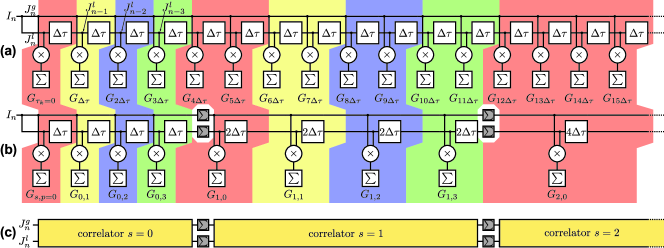
Figure 1: Hardware design of a linear correlator (a) in comparison with a multi-$\tau$ correlator (b). Panel (c) shows a schematic view of the multi-$\tau$ correlator, where the linear correlator building blocks are summarized by a single block. Corresponding channels are grouped with the same color. Global/undelayed ($g$) and local/delayed ($l$) inputs are located on the left. For autocorrelation, the global and local signal inputs to the $0$-th block ($J_{n}^{(g)}=J_{n}^{(l)}=I_{n}$) are identical. The $\boxed{\Delta\tau}$ blocks represent delay elements, the $\otimes$-blocks multipliers and the $\boxed{\Sigma}$-blocks accumulators.

III Hardware design

Here we describe how the hardware reuse scheme in the accompanying paper Ref. Mocsár et al., 2011 can be extended to accommodate many more input channels. Instead of the graphical tool used there, here we employed a low-level hardware description language to gain speed and flexibility. This enables us to fine-tune many parameters of the final design, e.g. operational speed, memory usage, logic resource consumption and routing between logic cells.

III.1 Single-Pixel Correlator

As shown in Figure 1, a typical correlator is made up from channels, each corresponding to a certain lag time and consisting of a multiplier, an accumulator and a delay element.

The idea of our implementation is to use one single channel circuit to calculate all channels within one multi-$\tau$ correlator. This is possible by serial processing of the lag time channels, since every channel’s hardware is identical.

The basic arithmetic operation of one channel is to multiply and accumulate (MAC). Therefore we can map its functionality onto a MAC unit which can be found on most FPGA architectures and which is considerably faster than using generic FPGA logic cells. Only about 100 of these can be found on typical FPGAs, precluding any approach with blocks consisting of several lag channels.

As only one circuit is used to process all channels, we use an internal memory block (block random access memory, BRAM) to store their state (i.e., the content of the accumulator and the delayed signal). We implement this circuit by decomposing it into five steps:

1. Load accumulator and delayed value of a channel from memory

2. Wait for memory access to complete

3. Multiply delayed with global signal

4. Add multiplication result to channel’s accumulator

5. Store counter and new delayed value to memory

To increase performance, these steps are executed in an interleaved manner for four channels simultaneously. This “pipelining” scheme is shown in TAB. 1. Our five pipeline steps are compatible with the internal pipelining of common MAC units.

Table 1: Interleaved pipeline of the linear correlator design with 8 channels.

cycle $c$	0	1	2	3	4	5	6	7	8	9	10	11	12	13	14	15
ch. 0	L	W	M	A	S				L	W	M	A	S				ch. 4
ch. 1		L	W	M	A	S				L	W	M	A	S			ch. 5
ch. 2			L	W	M	A	S				L	W	M	A	S		ch. 6
ch. 3				L	W	M	A	S				L	W	M	A	S	ch. 7

From one block to the next the delay time is doubled ($m=2$) in the multi-$\tau$ scheme, making the input data rate of block $s+1$ half that of block $s$. Hence we need to execute each block only half as often as its predecessor. Thus, a complete multi-$\tau$ correlator can be executed in only twice the run-time $\Delta t_{\text{lin}}$ of a single linear correlator block:

$$\overbrace{1\cdot\Delta t_{\text{lin}}}^{\text{1\textsuperscript{st} lin. corr.}}+\overbrace{\frac{1}{2}\cdot\Delta t_{\text{lin}}}^{\text{2\textsuperscript{nd} lin. corr.}}+\overbrace{\frac{1}{4}\cdot\Delta t_{\text{lin}}}^{\text{3\textsuperscript{rd} lin. corr.}}+\dots{\\ }\leq\sum_{n=0}^{\infty}\frac{1}{2^{n}}\cdot\Delta t_{\text{lin}}=2\cdot\Delta t_{\text{lin}}$$ (7)

A key requirement is that $\Delta t_{\text{lin}}$ is at most half the integration time $\tau_{\text{min}}$ of the input signal $I_{n}$.

As beforeMocsár et al. (2011), a scheduler guarantees that a linear correlator block $s$ is only executed after its predecessor $s-1$ has been executed twice. A counter $c=0,1,\ldots$ is incremented with every execution of any linear correlator block. The scheduler uses the following relations to determine which linear correlator block $s$ has to be executed at a given counter value $c$ (details see appendix):

$$s=0: \text{c}\bmod 2^{1} =0$$

$$s=1: \text{c}\bmod 2^{2} =3$$ (8)

$$s\geq 2: \text{c}\bmod 2^{s+1} =(2^{s}-3)$$

Figure 2(a) shows the solution of this relation for $c$ values from $0$ to $31$. In the binary representation of $c$ for a linear correlator block $s$ patterns are evident that can be used to implement the scheduler efficiently. As shown in TAB. 2 (for $S=8$ linear correlators), correlator block $s=0$ is executed whenever the last bit of $c$ is $0_{\text{b}}$, correlator $s=1$ is executed when the last two bits are $11_{\text{b}}$ and so forth. This scheme uses only simple comparison operations.

Table 2: Binary representation of counter $c$ that solves relations Eq. 8 for a given linear correlator block $s$. * denotes a don’t care condition.

	binary representation of counter $c$ that solves relation Eq. 8
lin. corr. $s$	$2^{8}$		$2^{7}$	$2^{6}$	$2^{5}$	$2^{4}$		$2^{3}$	$2^{2}$	$2^{1}$	$2^{0}$
0	*		*	*	*	*		*	*	*	0
1	*		*	*	*	*		*	*	1	1
2	*		*	*	*	*		*	0	0	1
3	*		*	*	*	*		0	1	0	1
4	*		*	*	*	0		1	1	0	1
5	*		*	*	0	1		1	1	0	1
6	*		*	0	1	1		1	1	0	1
7	*		0	1	1	1		1	1	0	1

Between two consecutive blocks $s-1$ and $s$, adder circuitry is inserted to sum up two subsequent input signal values $I_{s-1,n-1}$ and $I_{s-1,n}$. This is done for both the delayed/local as well as the undelayed/global signal, while they are processed in the pipeline.

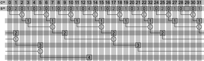
Figure 2: Block scheduling algorithm. The counter $c$ in the first row defines the current cycle. The second row shows the block $s$ that is processed in the corresponding cycle. Further below the order of processing is shown: When a block $s$ has been processed twice, the following block, $s+1$, can process the sum of the two preceding $s$-blocks.

The linear correlator as implemented here, together with its scheduler and the summation logic, is called correlation processing element (CorrPE). All channel data and intermediate summation results, the so-called pixel context, are stored in a dual-port BRAM which is associated with the CorrPE.

III.2 Multi-Pixel Correlator

The CorrPE described above is much faster than required to calculate the ACF for a single pixel in the SPAD array. Hence, we can reuse a single CorrPE for multiple pixels by switching between pixel contexts. This “pixel scheduler” uses a double-buffering strategy. While a CorrPE operates on the current context, the previous context is exchanged with the next context to be processed. The pixel contexts are stored in external background memory (SRAM), because they exceed the capacity of the internal memory. In Figure 3 we illustrate how we reuse one CorrPE for several pixels in comparison to a naïve implementation using one CorrPE per pixel.

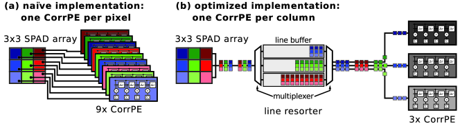
Figure 3: Comparison of a naïve implementation (a: one correlator per pixel) and an optimized implementation (b: reuse CorrPEs for several pixels) of a multi-pixel multi-$\tau$ correlator for a $3\times 3$ SPAD array.

In addition to the channel data, the cycle counter $c$ and an accumulator for the local and the global input signals have to be saved. The latter are used for normalization and cross-correlation.

A single CorrPE is used to process an entire column (ACFs of $n_{y}=32$ pixels) of our SPAD array. To handle the full $n_{x}\times n_{y}$ array of pixels, we instantiate $n_{x}=32$ CorrPEs in parallel. An overview of this scheme is shown in Figure 4. A “data acquisition” circuit communicates with the SPAD array and provides the image data for the correlators. As the image data are streamed out row by row, and each of the $n_{x}$ CorrPEs is only processing data from one specific context (i.e. a specific row), the remaining pixels have to be buffered in 32 FIFOs (first-in first-out memory buffer) localized in external RAM.

In addition our design contains two USB 2.0 interfaces. One is used to send the raw data stream from the SPAD array to the computer, which allows further data processing. We also use these raw data to verify our correlator design. Via the second interface, intermediate and final results from the correlators are transferred to the host computer. The intermediate results allow implementing a live view of the ongoing calculation of the ACFs.

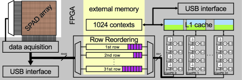
Figure 4: System layout and data path - from data acquisition to correlation. One USB interface is used to stream the raw images, the other for streaming (intermediate) results. The first level cache (L1, double buffered) is used to hold the context of the currently processed pixel. FIFOs for row resorting and for context storage use external memory.

III.3 ACF Normalization

The intensity values in the denominator of Eq. 3 are typically obtained from monitor channels $M_{\tau_{k}}$, which accumulate the total photon count at a given lag time $\tau_{k}$. In contrast to other implementations, we use only one monitor $M_{0}$ (input signal accumulator) per multi-$\tau$ correlator. Symmetric normalization (see also Eq. 3) yields the following:

$$\hat{g}_{\text{sym,\mbox{multi-$\tau$}\ }}(\tau_{s,p})=\frac{G_{\tau_{s,p}}}{2^{s}}\cdot\frac{T}{M_{0}\cdot M_{\tau_{s,p}}}$$ (9)

After measuring $T$ samples, the number of samples that have propagated through the correlator to a distinct channel $(s,p)$ is $T-\tau_{s,p}$. Under the assumption that $I_{n}$ is a stationary random process and that $T>\tau_{s,p}$, the per-channel monitors $M_{\tau_{s,p}}$ can be estimated in the following manner:

$$M_{\tau_{s,p}}=M_{0}\cdot\frac{T-\tau_{s,p}}{T}.$$ (10)

This normalization and model fitting is done on the host computer, since floating-point arithmetic cannot be implemented efficiently on an FPGA. Although the correlation on the FPGA and the normalization on the host computer can easily be done in real time, the fits in most cases cannot. Usually a single curve fit takes tens of milliseconds, thus fitting all $1024$ ACFs would amount to $\geq 10\,\mathrm{s}$ additional computing time; but this still allows to display fit parameter maps (images) within an acceptably short delay. In current imaging FCS software systemsSankaran et al. (2010) the data are loaded and correlated on the host computer, which for a measurement of typically $10\,\mathrm{s}$ takes $\geq 10\,\mathrm{min}$ for $1024$ pixels at the frame rate of our sensor.

To show that the estimation in Eq. 10 yields good results, we simulated different correlator types in software. The results for a direct estimation of the ACF using Eq. 3 (green), a multi-$\tau$ correlator with a monitor channel per lag (blue) and our estimation (magenta) can be seen in Figure 5, where the data in (a) and (b) were obtained by correlating the input signal $I(t)=1+\sin(2\pi t/(1.51\cdot 10^{-4}))$ for which the exact ACF is known to be $g^{\text{(theoretical)}}(\tau)=1+\cos(2\pi\tau/(1.51\cdot 10^{-4}))$ (time $t$ and lags $\tau$ are unit free). The data in Figure 5(c) was created by simulating a $T_{\text{sim}}=1\,\mathrm{s}$ long FCS experiment with one diffusing speciesnot (b). It was computed with our FCS simulation software described in Ref. Wocjan et al., 2009. Further details on the simulation code are shown in the appendix.

For short lags the estimated ACFs resemble the theoretical curves quite well. Multi-$\tau$ correlators have an increased absolute error for longer lags, which is due to the averaging described in Eq. 6. This can be seen especially in the case of the sine wave signal. The multi-$\tau$ estimates can still be used for FCS experiments, as here the ACFs usually decay to 1 (white noise) for large lag times, and thus the systematic error drops to zero again (for a detailed discussion of this, see e.g. Ref. Kojro et al., 1999). For $\tau\gtrsim T_{\text{sim}}/10$, multi-$\tau$ correlators show additional systematic deviations from the theoretical curve and from the direct estimation, because the channels are not averaged over sufficiently many samples to yield reliable results. Here the multi-$\tau$ implementation with multiple monitor channels performs better due to the better estimation of the normalization factor $M_{\tau_{s,p}}$.

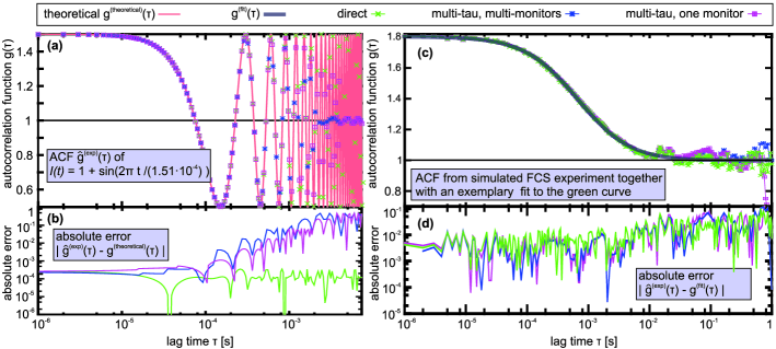
Figure 5: Simulation results for different implementations of multi-$\tau$ correlators: The left panels (a,b) show simulations for a sine wave input signal $I(t)=1+\sin(2\pi t/(0.151\,\mathrm{ms}))$. The simulations on the right (c,d) were created using an FCS simulation. The top graphs (a,c) are estimates of the autocorrelation function using direct correlation from Eq. 3 (green), a multi-$\tau$ correlator with one monitor channel per lag time (blue) and our estimated normalization from Eq. 10 (magenta). Graph (a) also shows the theorectical ACF $g^{\text{(theoretical)}}(\tau)=1+\cos(2\pi\tau/(0.151\,\mathrm{ms}))$ for the sine signal (light red). The lower graphs (b,d) show the absolute deviation of the estimates from $g^{\text{(theoretical)}}(\tau)$ (b) and from a fit to the curves (d). The parameters resulting from the fit in (c) are the same within $<2.5\%$ for all three estimates.

III.4 Crosscorrelation (CCF)

Our design can also calculate cross-correlation:

$$g^{(x,y)}(\tau)=\frac{\left\langle{I^{(x)}(t)\cdot I^{(y)}(t+\tau)}\right\rangle_{t}}{\left\langle{I^{(x)}(t)}\right\rangle_{t}\cdot\left\langle{I^{(y)}(t)}\right\rangle_{t}}$$

between two input signals $I^{(x)}(t)$ and $I^{(y)}(t)$ at the local $J^{\text{(l)}}$ and global $J^{\text{(g)}}$ inputs of the CorrPE (see Figure 1 where both signals are tied to $I(t)$ for ACF calculation). This changes the multi-$\tau$ estimator Eq. 9 to:

$$\hat{g}^{\text{(CCF)}}_{\text{sym,\mbox{multi-$\tau$}\ }}(\tau_{s,p})=\frac{G_{\tau_{s,p}}}{2^{s}}\cdot\frac{T}{M^{(g)}_{0}\cdot M^{(l)}_{\tau_{s,p}}}$$ (11)

Here the normalization uses the monitors $M^{(g)}_{0}$ for the global and $M^{(l)}_{0}$ for the local signal ($M^{(l)}_{\tau_{s,p}}=M^{(g)}_{0}\cdot(T-\tau_{s,p})/T$). For autocorrelation (see above) only one monitor channel is needed, as $M_{0}=M^{(g)}=M^{(l)}$.

IV Performance & Implementation Details

The complete design is implemented in two Virtex-II Pro FPGAs (XC2VP40, Xilinx, http://www.xilinx.com/, San Jose, USA), on a LASP development boardNiclass et al. (2008). One FPGA is used for data acquisition and line reordering, while the other one is used to implement the correlators. The total resource consumption within the second FPGA is around $80\%$. Using this hardware platform, there are currently $P=8$ channels within each of the $S=14$ linear correlator blocks.

In Eq. 7 we showed that the complete multi-$\tau$ correlator can be executed within twice the time needed for the first linear correlator block, so we devote half of the execution time to the first linear correlator and the rest to the remaining blocks. Therefore a new input sample can be accepted only once every $2\Delta t_{\text{lin}}$. Here $\Delta t_{\text{lin}}=2P+3\,\mathrm{cycles}$ is the time needed to process a new input sample $I_{n}$ in the first linear correlator block. The $3$ additional cycles are used for data hand over to the next block.

The CorrPEs run with a clock frequency of $144\,\mathrm{MHz}$, which corresponds to an execution time of $264\,\mathrm{ns}=2\Delta t_{\text{lin}}$. This is the minimum timespan between two subsequent samples, if no pixel multiplexing is used. Hence, our current FPGA platform can calculate $32$ different ACFs or CCFs with a minimum lag time of $264\,\mathrm{ns}$, which is comparable to the $100\,\mathrm{ns}$ designs presented in Ref. Jakob et al., 2006 and more recently in Ref. Mocsár et al., 2011. Trading time resolution for more correlation functions, we can process all $1024$ pixels of the SPAD array at a frame rate of $100\,\mathrm{kfps}$ in real time.

To estimate the memory consumption of our design, we first look at the pixel context, which consists of $128$ words of $64$ bits each. TAB. 3 shows a detailed memory layout. Sixteen of the upper $32\,\mathrm{bits}$ of the raw accumulators store the current value of the delay registers $J^{(l)}_{s,p}$. The lower $32\,\mathrm{bits}$ contain the accumulator $G_{\tau_{s,p}}$. The monitor channels are $32\,\mathrm{bits}$ each. Data handover between consecutive blocks (accumulated local and global signals) is done via $16\,\mathrm{bit}$-wide memory areas, which is sufficient for $S\leq 16$. Since in the later linear correlators the accumulated input signals $I_{s,n}$ are multiplied, the sums $G_{\tau_{s,p}}$ and also the $I_{s,n}$ can get relatively large and may not fit in the $32\,\mathrm{bit}$ memory locations available. However, for our FCS application we estimate that the word sizes used are sufficient, since the per-pixel input event rate is limited. For a deeper discussion of this topic, see Ref. Hoppe et al., 2001.

data word	usage
$0...111$	delay register $J^{(l)}_{s,p}$ and raw accumulator values $G_{\tau_{s,p}}$
$112$	status counter $c$
$113...125$	intermediate results for accumulated input signals $I_{s,n}$
$126$	global monitor channel $M^{(g)}_{0}$
$127$	local monitor channel $M^{(l)}_{0}$

Table 3: Memory layout of a pixel context

For our $32\times 32$ pixel SPAD array the pixel contexts are stored in $32\cdot 32\cdot 128\cdot 64\,\mathrm{bits}=512\,\mathrm{KBytes}$ of external SRAM. A second SRAM stores the $256\,\mathrm{KBytes}$ used for the FIFOs ($2048$ entries each) that hold the pixel data until they are processed.

The correlator design is implemented in VHDL (very high speed integrated circuit hardware description language). It can be configured via generics (a VHDL feature). Thus we can reuse our design for different needs (e.g. for different sensor sizes and frame rates). We expect our design to show a significant increase in performance when implemented on newer FPGA generations (e.g. Virtex 5 or Virtex 6 from Xilinx).

To ensure the functional correctness of the designed correlator, a simulation of the hardware was tested using random input data. The outcome was compared to the results of a software implementation of the multi-$\tau$ correlator using the same data set. Both yielded exactly the same results. The comparison was also done using real experimental data from the SPAD array. Again, both results were identical.

To demonstrate the functionality of the whole system, we tested the design using the SPAD array to record an LED connected to a sine wave generator set to $2.5\,\mathrm{kHz}$. Figure 6 shows the results of this measurement. A fit to the data recovered the chosen frequency.

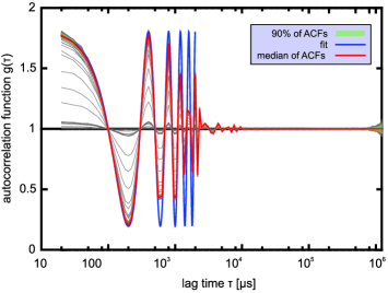
Figure 6: Distribution of 992 (gray) ACFs taken by our sensor (first 31 columns only), exposed to a 630 nm LED sine-modulated with a frequency of $2.5\,\mathrm{kHz}$. The correlator was running for $1.2\,\mathrm{s}$ (131072 samples at $\tau_{\text{min}}=10\,\mathrm{\mu s}$). The gray curves with significantly lower amplitude are due to hot pixels of the SPAD array; since these SPADs fire randomly, the corresponding correlation amplitude is decreased. The median, which tends to be less sensitive towards outliers than the mean, is shown in red. The theoretical model $g^{\text{(theoretical)}}(\tau)=1+A\cdot\cos(2\pi f\cdot\tau)$ is fitted against the median in the interval $\left[10\,\mathrm{\mu s},1\,\mathrm{ms}\right]$, and is shown until $\tau=2\,\mathrm{ms}$. The fit yields a frequency of $(2502\pm 4)\,\mathrm{Hz}$. The fanning out of the curve at high values of $\tau$ is due to unfilled correlator channels. Compare also Figure 5(a).

V Conclusion

In this paper we presented the implementation of an FPGA-based multi-$\tau$ correlator design that can calculate $1024$ correlation functions in real time at a minimum lag time of $10\,\mathrm{\mu s}$. To our knowledge this is the largest number of real-time multi-$\tau$ correlators implemented so far in a single device. The minimum lag time of $10\,\mathrm{\mu s}$ in our design is considerably longer than that of currently available hardware correlators (e.g. from ALV GmbH, Langen, Germany or correlator.com, Bridgewater, USA and Ref. Magatti and Ferri, 2003). However, those are limited to at most $32$ auto-correlators.

We use our design to correlate the output of a single-photon avalanche diode array used as image sensor. This combination will allow us to perform imaging fluorescence correlation spectroscopy at sufficiently fast time scales to resolve even the motion of small molecules in solution and living cells.

Our design is flexible, so beside estimating ACFs, temporal cross-correlation functions of different pixelsDertinger et al. (2007); Colyer et al. (2010) or multiple colorsBestvater et al. (2010) (using spectrally resolved detectors) can also be calculated.

Appendix A Relation Eq. 8

By definition, Eq. 8 can be rewritten in the following manner, with $C_{s}$ containing the cycles in which the linear correlator $s$ is processed:

$$C_{0} = \left\{c=n\cdot 2^{1}+0\mid c,n\in\mathbb{N}_{0}\right\}$$

$$C_{1} = \left\{c=n\cdot 2^{2}+3\mid c,n\in\mathbb{N}_{0}\right\}$$

$$C_{s} = \left\{c=n\cdot 2^{s+1}+2^{s}-3\mid c,n\in\mathbb{N}_{0}\right\}\forall s\geq 2$$

It remains to show that $C_{p}\cap C_{q}\forall p,q\in\mathbb{N}_{0}$, $p\neq q$. Obviously $C_{0}\cap C_{s}\;\forall s\in\mathbb{N}$, $k,l\in\mathbb{N}_{0}$:

$$C_{1}\cap C_{2} =\varnothing$$

$$\Rightarrow k\cdot 2^{2}+3 \neq l\cdot 2^{3}+1$$

$$\Leftrightarrow \underbrace{k}_{\in\mathbb{N}_{0}} \neq\underbrace{2l}_{\in\mathbb{N}_{0}}-\underbrace{\frac{1}{2}}_{\in\mathbb{Q}}$$

$$\Rightarrow \surd$$

Without limitations let $r<s$; $\forall r,s\in\mathbb{N}_{0}$; $r,s\geq 2$; $k,l\in\mathbb{N}_{0}$:

$$C_{r}\cap C_{s} =\varnothing$$

$$\Rightarrow k\cdot 2^{r+1}+2^{r}-3 \neq l\cdot 2^{s+1}+2^{s}-3$$

$$\Leftrightarrow \underbrace{k}_{\in\mathbb{N}_{0}} \neq\underbrace{l\cdot 2^{s-r}+2^{s-r-1}}_{\in\mathbb{N}_{0}}-\underbrace{\frac{1}{2}}_{\in\mathbb{Q}}$$

$$\Rightarrow \surd$$

Appendix B FCS Simulation & Fits

To test different types of autocorrelators, we used our FCS simulation program described in Ref. Wocjan et al., 2009. It simulates the 3D trajectories

$$\vec{r}_{i}(t),t=0...T_{\text{sim}},i=1..K$$

of a set of $K$ fluorescing particles performing a random walk in which each 1D step is drawn from a zero-centered Gaussian distribution with width

$$\sigma_{\text{jump}}=\sqrt{2D\cdot\Delta t_{\text{sim}}}.$$

Here $D$ is the given diffusion coefficient and $\Delta t_{\text{sim}}$ is the simulation time step. We use a Gaussian approximation for the focal illumination and detection volume:

$$h(x,y,z)=\exp\left(-2\cdot\frac{x^{2}+y^{2}}{w_{\rm xy}^{2}}-2\cdot\frac{z^{2}}{\gamma^{2}w_{\rm xy}^{2}}\right),$$

where $w_{\rm xy}$ is the lateral width of the profile, $\gamma=w_{\rm z}/w_{\rm xy}$ is its aspect ratio and $w_{\rm z}$ is its length. The program then estimates the expected number of photons $\overline{N}_{\rm phot}(t)$ detected during each simulation time step $[t,t+\Delta t_{\rm sim}]$:

$$\overline{N}_{\rm phot}(t)=\overline{N}_{0}\cdot\Delta t_{\rm sim}\cdot\sum\limits_{i=1}^{K}q_{\rm f}\cdot q_{\rm det}\cdot h(\vec{r}_{i}(t))^{2}.$$

Here $\overline{N}_{0}$ is the maximum number of detected photons per fluorophore and time step, while $q_{\rm f}$ and $q_{\rm det}$ are the quantum efficiencies of fluorescence and detection. To account for the counting statistics in the SPADs, the number of photons $N_{\rm phot}(t)$ actually detected during a simulation time step is calculated by drawing a random number from a Poissonian distribution with average $\overline{N}_{\rm phot}(t)$.

The time series created by the simulation is then fed into the three different autocorrelator software implementations: (a) direct estimation, (b) multi-$\tau$ with one monitor channel and (c) multi-$\tau$ with multiple monitor channels. The latter two (b, c) simulate the complete structure of a multi-$\tau$ correlator. In correlator (b) we use one single monitor channel, which counts the incoming photons only and then uses Eq. 10 for the normalization. In the correlator (c) we use one monitor channel per correlator lag which counts the photons actually processed by each lag.

The simulation parameters for the data in Figure 5 are summarized in TAB. 4. The average photon count rate in the simulations was $\langle I(t)\rangle\approx 157.4\,\mathrm{kHz}$ which is – due to the chosen detection efficiency $q_{\rm det}=0.5$ – about a factor of 5 higher than what would be expected from a standard confocal FCS setup. This way the signal to noise ratio is high enough to visualize easily artifacts introduced by the correlator implementation. Figure 7 shows an example of a time trace $N_{\rm phot}(t)/\Delta t_{\rm sim}$ generated by our simulation.

$T_{\rm sim}$	duration of simulation	$1\;\mathrm{s}$
$\Delta t_{\rm sim}$	simulation time step	$1\;\mathrm{\mu s}$
$K$	number of walkers	$1576$
$V_{\rm sim}$	simulation volume	$524\,\mathrm{\mu m^{3}}$
$c$	concentration of simulated particles	$5\,\mathrm{nM}$
$D$	diffusion coefficient	$20\,\mathrm{\mu m^{2}/s}$
$\overline{N}_{0}$	absorbed photons per molecule	$4.2\cdot 10^{6}\,\mathrm{s^{-1}}$
$w_{\rm xy}$	lateral width of excitation profile	$0.325\,\mathrm{\mu m}$
$q_{\rm f}$	fluorescence quantum yield	$0.8$
$q_{\rm det}$	detection efficiency	$0.5$
$\gamma$	focal aspect ration	$6$
$S$	number of linear correlator blocks	$20$
$P$	number of channels per block	$16$
$m$	lag time ratio between blocks	$2$

Table 4: Simulation parameters for the FCS simulation yielding the results, displayed in Figure 5.

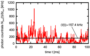
Figure 7: Typical photon count time trace $N_{\rm phot}(t)/\Delta t_{\rm sim}$ generated by our simulation

The resulting ACFs were fitted to a standard 3D FCS model functionKrichevsky and Bonnet (2002):

$$g^{\text{(fit)}}(\tau)=\frac{1}{N}\cdot\left(1+\frac{\tau}{\tau_{D}}\right)^{-1}\cdot\left(1+\frac{\tau}{\gamma^{2}\tau_{D}}\right)^{-1/2}$$

with the average particle number $N$ in the effective focal volume $V_{\rm eff}=\pi^{3/2}\cdot\gamma\cdot w_{\rm xy}^{3}$ and the diffusion decay time $\tau_{D}={w^{2}_{\rm xy}}/{4D}$. The fits were performed using a Levenberg-Marquardt least squares fitting routine.

References & Footnotes

References

- Magde, Elson, and Webb (1974a) D. Magde, E. L. Elson, and W. W. Webb, Biopolymers 13, 1 (1974a).
- Magde, Elson, and Webb (1974b) D. Magde, E. L. Elson, and W. W. Webb, Biopolymers 13, 29 (1974b).
- Krichevsky and Bonnet (2002) O. Krichevsky and G. Bonnet, Reports on Progress in Physics 65, 251 (2002).
- Mocsár et al. (2011) G. Mocsár, B. Kreith, J. Buchholz, J. W. Krieger, J. Langowski, and G. Vámosi, Review of Scientific Instruments ?, ? (2011).
- Kannan et al. (2007) B. Kannan, L. Guo, T. Sudhaharan, S. Ahmed, I. Maruyama, and T. Wohland, Analytical Chemistry 79, 4463 (2007).
- Dross et al. (2009) N. Dross, C. Spriet, M. Zwerger, G. Müller, W. Waldeck, and J. Langowski, PLoS ONE 4, e5041 (2009).
- Wohland et al. (2010) T. Wohland, X. Shi, J. Sankaran, and E. H. K. Stelzer, Optics Express 10, 10627 (2010).
- not (a) The single SPADs of Radhard2 have a photon detection probability of around at a wavelength of . The fill factor of the array is around .
- Carrara et al. (2009) L. Carrara, C. Niclass, N. Scheidegger, H. Shea, and E. Charbon, in ISSCC, IEEE International Solid-State Circuits Conference (2009) pp. 40–41.
- Schätzel (1990) K. Schätzel, Quantum Opt. 2, 287 (1990).
- Schätzel (1985) K. Schätzel, Institute of Physics Conference Series 77, 175 (1985).
- Kojro et al. (1999) Z. Kojro, A. Riede, M. Schubert, and W. Grill, Review of Scientific Instruments 70, 4487 (1999).
- Sankaran et al. (2010) J. Sankaran, X. Shi, L. Ho, E. Stelzer, and T. Wohland, Optics Express 18, 25468 (2010).
- not (b) The diffusion coefficient was (corresponding to an intermediately sized protein in water), the simulation timestep of the random walk, as well as the minimum lag time were . There were around particles in the effective measurement volume on average.
- Wocjan et al. (2009) T. Wocjan, J. Krieger, O. Krichevsky, and J. Langowski, Phys. Chem. Chem. Phys. 11, 10671 (2009).
- Niclass et al. (2008) C. Niclass, C. Favi, T. Kluter, M. Gersbach, and E. Charbon, in ISSCC, IEEE International Solid-State Circuits Conference (IEEE, 2008) pp. 44–594.
- Jakob et al. (2006) C. Jakob, A. Schwarzbacher, B. Hoppe, and R. Peters, in Irish Signals and Systems Conference, 2006. IET (IET, 2006) pp. 99–103.
- Hoppe et al. (2001) B. Hoppe, H. Meuth, M. Engels, and R. Peters, in IEEE Proceedings Circuits, Devices and Systems, Vol. 148 (IET, 2001) pp. 267–271.
- Magatti and Ferri (2003) D. Magatti and F. Ferri, Review of Scientific Instruments 74, 1135 (2003).
- Dertinger et al. (2007) T. Dertinger, V. Pacheco, der Hocht Iris von, R. Hartmann, I. Gregor, and J. Enderlein, ChemPhysChem 8, 433 (2007).
- Colyer et al. (2010) R. A. Colyer, G. Scalia, I. Rech, A. Gulinatti, M. Ghioni, S. Cova, S. Weiss, and X. Michalet, Biomedical Optics Express 1, 1408 (2010).
- Bestvater et al. (2010) F. Bestvater, Z. Seghiri, M. S. Kang, N. Gröner, J. Y. Lee, I. Kang-Bin, and M. Wachsmuth, OPTICS EXPRESS 18, 23818 (2010).