Searching for Gravitational Waves with a
Geostationary Interferometer

Abstract

We analyze the sensitivities of a geostationary gravitational wave interferometer mission operating in the sub-Hertz band. Because of its smaller armlength, in the lower part of its accessible frequency band ($10^{-4}-2\times 10^{-2}$ Hz) our proposed Earth-orbiting detector will be less sensitive, by a factor of about seventy, than the Laser Interferometer Space Antenna (LISA) mission. In the higher part of its band instead ($2\times 10^{-2}-10$ Hz), our proposed interferometer will have the capability of observing super-massive black holes (SMBHs) with masses smaller than $\sim 10^{6}$ M_⊙. With good event rates for these systems, a geostationary interferometer will be able to accurately probe the astrophysical scenarios that account for their formation.

1 Introduction

The quest for the direct observation of gravitational radiation is one of the most pressing challenges in the physics of this century. Predicted by Einstein shortly after formulating his general theory of relativity, gravitational waves (GW) will allow us to probe regions of space-time otherwise unobservable in the electromagnetic spectrum [1]. Although we have excellent indirect evidence of their existence through their effects on the orbital evolution of binary systems containing pulsars, we have not been able yet to directly detect them. Several ground-based gravitational wave detectors have been operational for awhile, and only recently they have been able to identify the most stringent upper limits to date for the amplitudes of the radiation expected from several classes of sources [2, 3, 4, 5]. Next generation of Earth-based interferometers and pulsar-timing experiments [6], as well as newly conceived space-born detectors [7] are expected to achieve this goal.

Ground-based interferometers operate in the frequency band whose lower limit is at about $10$ Hz, mainly because of the large seismic and gravity-gradient noises below this frequency cut-off. Since the mHz region is potentially very rich in gravitational wave sources, the most natural way to observe them is to build and operate a space-borne detector. The most notable example of a space interferometer, which has been under study for several years jointly by scientists in the United States of America and in Europe, is the Laser Interferometer Space Antenna (LISA) mission. By relying on coherent laser beams exchanged between three remote spacecraft forming a giant (almost) equilateral triangle, LISA aimed to detect and study cosmic gravitational waves in the $10^{-4}-1$ Hz band.

Although over the years only a few space-based detector mission concepts have been considered as alternatives to the LISA mission (with ASTROD [8], DECIGO [9], and OMEGA [10] being the most notable examples), starting in 2011 (with the ending of the NASA/ESA partnership for flying LISA) more mission concepts have appeared in the literature [11]. Their goals are to meet most (if not all) the LISA scientific objectives (highlighted in the 2010 Astrophysics Decadal Survey New Worlds, New Horizons (NWNH) [12]) at a lower cost.

In this context, motivated by the interest of the Brazilian Space Agency to pursue the development and launch of several geostationary satellites, we decided to analyze the scientific capabilities offered by a geostationary gravitational wave interferometer, henceforth called GEOGRAWI. GEOGRAWI was one of the alternative concepts to the LISA mission submitted in response to NASA’s Request for Information # NNH11ZDA019L [13]. A detailed analysis of all the submitted projects and a final study report can be found in [11]. Among them, a proposal by Sean T. McWilliams explores a mission concept very similar to the one discussed in this paper [14, 15] called GADFLI. His concept and the one proposed by us, though strikingly similar, were nonetheless independently developed and submitted.

GEOGRAWI, like LISA, has three identical spacecraft interchanging coherent laser beams and forming an (almost) equilateral triangle. However, by being in a geostationary orbit, its accessible frequency band changes to about ($10^{-3}-10$ Hz). It is worth noting that, although our interferometer reminds that of the OMEGA mission (proposed by R. Hellings [10] about 15 years ago), it is in fact very different from it. The OMEGA spacecraft were six in total, with two at each vertex of a geocentric equilateral triangle of side equal to one million kilometers. Cost of the launching vehicle as well as challenges in performing the phase measurements associated to the large relative velocities between the spacecraft make OMEGA quite different from GEOGRAWI.

The astrophysical sources that GEOGRAWI is expected to observe within its operational frequency band include extra-galactic massive and super-massive black-hole coalescing binaries, the resolved galactic binaries and extra-galactic coalescing binary systems containing white dwarfs and neutron stars, a stochastic background of astrophysical and cosmological origin, and possibly more exotic sources such as cosmic strings. With GEOGRAWI we will be able to test Einstein’s theory of relativity by comparing the waveforms detected against those predicted by alternative relativistic theories of gravity, and also by measuring the number of independent polarizations of the detected gravitational wave signals [16].

Since the sensitivities of the geostationary interferometers we considered (see section 2 below) are degraded by their shorter armlength in the frequency region ($10^{-4}-2\times 10^{-2}$) Hz, it will be impossible for them to detect the zero-order cyclic spectrum of the white dwarf-white dwarf galactic binary confusion noise. However, as pointed out in [17], the periodic nature of the galactic background signal in the data of an interferometer rotating around the Sun will contain higher-order “cyclic spectra”, which are in principle not affected by the instrumental noise (if this is stationary). This implies that we could still detect the so-called “confusion noise”, and infer properties of the distribution of the white-dwarf binary systems present in our galaxy [17].

In this article we pay particular attention to super-massive black holes, which are the main sources of GWs for interferometers operating at frequencies below $1$ Hz. We show that GEOGRAWI will be able to detect a large number of SMBHs at very high redshifts, and that a significant fraction of them will have masses smaller than $10^{6}$ M_⊙ as a consequence of its improved sensitivity at higher frequencies.

This paper is organized as follows. In section 2 we provide a description of the mission and a system noise analysis in order to evaluate the sensitivities of the Time-Delay Interferometric (TDI) [18] response $X$. It is in this section and in A where we also emphasize that additional instrumental techniques over those baselined for LISA will need to be implemented in order to achieve the derived sensitivities. These are estimated for three different on board subsystem configurations of GEOGRAWI, which we refer to as Geostationary 1 (GEO1), Geostationary 2 (GEO2) , and Geostationary 3 (GEO3). We note that the GEO1 configuration has a reduced sensitivity over that of LISA by a factor of about $70$ in the lower part of its accessible frequency band ($10^{-4}-2\times 10^{-2}$ Hz). On the other hand, in section 3 we discuss possible sources of gravitational waves observable by GEOGRAWI in the higher-part of its band ($2\times 10^{-2}-10$ Hz). Particular attention is devoted to SMBHs and we show that the number of observable signals from such systems, with masses smaller than or equal to $10^{6}$ M_⊙, would be significant. Finally, in Section 4 we provide a summary of our work and conclusions.

2 Mission Design and Interferometer Sensitivities

Our proposed space-based detector entails three spacecraft in geostationary orbit, forming an equilateral triangle with armlength of about $73,000$ km. Since the constellation plane coincides with the Earth equatorial plane, each spacecraft will need to be spherical and entirely covered with photo-voltaic cells. This will allow each spacecraft to be continuously powered (without the need of rotating it as the Earth orbits around the Sun) and maintain a high-level of thermal stability. It should be noticed also that the inclination ($23.5^{0}$) of the Earth equatorial plane with respect to the ecliptic will prevent (i) Sun light from contaminating the optics of the spacecraft during most of the interferometer orbital period around the Sun, and (ii) spacecraft occultation by the Earth. In proximity of the equinoxes, however, these properties will no longer be true and, in order to avoid these short-period operation interruptions, onboard electric power and Sun-light filters will need to be used. Sun-light filters needed for this purpose have already been developed for the OMEGA mission, which requires their usage at all times in its geocentric trajectory [19].

As the Sun and the Moon will exercise gravitational perturbations on each spacecraft (resulting into a long-term orbital drift), in order to maintain orbital stability and small inter-spacecraft relative velocities, each spacecraft will need to implement “station-keeping” [20]. This is required not only for keeping the constellation in a stable configuration, but most importantly for relying on a phase-meter design that does not need to accommodate large relative frequency offsets, making it significantly less noisy (see A). By taking the nominal value of $2\ {\rm m/s/year}$ for the “East-West” acceleration perturbation [20] acting on the spacecraft (which is responsible for the spacecraft relative velocities), it is easy to show that, in order to maintain their maximum velocities smaller than about a few decimeters per second, the station-keeping operation will need to be applied about once per week (see A).

In order to estimate the TDI sensitivities of our geostationary GW interferometer detector, we have relied on some LISA study documents [7, 21]. This allowed us to derive a break-down estimate of the various noise sources affecting the TDI observables and compute the TDI sensitivities of a geostationary interferometer under the following three different on-board subsystem configurations:

1. Some of the onboard science payload components (the laser, the optical telescope, the inertial reference sensor) are assumed to be equal and have a similar noise performance of those planned to be flown onboard the LISA mission. Other subsystems are regarded to have a noise performance that results in a high-frequency noise spectrum that is essentially determined by the photon-counting statistics. It should be emphasized, however, that our assumed noise performance in the high-frequency region of the accessible band requires additional instrumental developments over those baselined for the LISA mission [22, 23, 24]. In order to better understand this point we refer the reader to A where it is discussed somewhat at length. We will refer to this configuration as “Geostationary 1” (or GEO1).

2. The output power of the onboard lasers and the size of the optical telescopes are assumed to be equal to those of the LISA mission, while the noise performance of the gravitational reference sensors (GRS) is taken to be a factor of ten worse than that of the GRSs planned for the LISA mission. The remaining noises are as in the GEO1 case, and this configuration will be referred to as “Geostationary 2” (or GEO2).

3. The noise performance of each GRS is taken a factor of ten worse than that of the GRS planned for the LISA mission, the output power of the lasers is assumed to be a factor of $10$ smaller than that of the lasers onboard LISA, the diameter of the optical telescopes has been reduced by a factor of $\sqrt{10}$ over that of the LISA telescopes, and the remaining noises are assumed to be equal to those for the GEO1 configuration. This configuration will be called “Geostationary 3” (or GEO3).

The sensitivity of an interferometer detector of gravitational radiation has been traditionally taken to be equal to (on average over the sky and polarization states) the strength of a sinusoidal GW required to achieve a signal-to-noise ratio of $5$ in a one-year integration time, as a function of Fourier frequency. For sake of simplicity we will limit the derivation of the sensitivities of the three geostationary configurations described above to only the “X” TDI combination, as those for the other TDI combinations can be inferred by properly scaling those for $X$. To this end we will be following the same procedure described in [27, 28], and rely on the following expression for the power spectrum of the noises affecting the $X$ combination (see Figure 1)

$$S_{X}(f)=[8\sin^{2}(4\pi fL)+32\sin^{2}(2\pi fL)]S^{pm}_{y}(f)+16\sin^{2}(2\pi fL)\ S^{op}_{y}(f)\ ,$$ (1)

where $S^{pm}_{y}(f)$ is the spectrum of the relative frequency fluctuations due to each proof mass, and $S^{op}_{y}(f)$ is the spectrum of optical path (mainly shot and beam pointing) noise. Both these noises have been regarded as the main limiting noise sources for LISA [7, 28], and will be treated as such for our geostationary interferometer configuration (see A for details). It should be acknowledged, however, that the dramatic reduction in optical path noise assumed in this article reflects the implementation of additional instrumental techniques over those baselined for LISA [22, 23, 24].

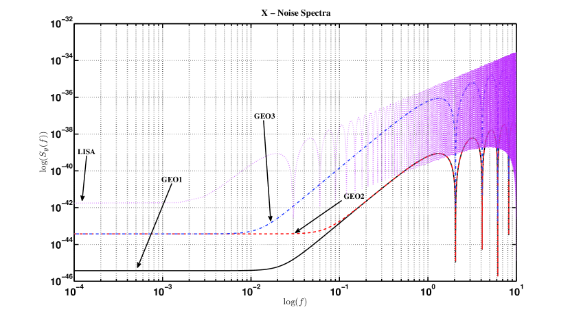
Figure 1: Noise spectra for the $X$ time-delay interferometric combination for the three on-board hardware configurations (I), (II), and (III) (see text). The varying depths of the minima in the high-frequency range is an artifact of numerically calculating these functions at discrete frequencies

The numerical expressions for the spectra $S^{pm}_{y}(f)$, $S^{op}_{y}(f)$ associated to the LISA mission were provided in [28] and they are equal to $S^{pm}_{y}(f)|_{LISA}=2.5\times 10^{-48}\ [f/1Hz]^{-2}\ {\rm Hz}^{-1}$ and $S^{op}_{y}(f)|_{LISA}=1.8\times 10^{-37}[f/1Hz]^{2}\ {\rm Hz}^{-1}$. The configurations (I), (II) and (III) discussed above require appropriate scaling factors of these noise levels, and they are given in Table 1 (also see A for detail analysis of the other noise sources).

Mission	$S^{op}_{y}|_{LISA}$	$S^{pm}_{y}|_{LISA}$
LISA	$1$	$1$
Geo. 1	$(L_{GEO}/L_{LISA})^{2}$	$1$
Geo. 2	$(L_{GEO}/L_{LISA})^{2}$	$10^{2}$
Geo. 3	$(L_{GEO}/L_{LISA})^{2}\times 10^{3}$	$10^{2}$

Table 1: Noise spectra scaling factors as functions of the different instrument configurations analyzed. See text for more details.

Gravitational wave sensitivity is the wave amplitude required to achieve a given signal-to-noise ratio. We calculate it in the conventional way, requiring a signal-to-noise ratio of $5$ in a one year integration time: $5\ \sqrt{S_{X}(f)\ B}$/(root-mean-squared gravitational wave response of $X$). The bandwidth, $B$, was taken to be equal to one cycle/year (i.e. $3.17\times 10^{-8}$ Hz), while the root-mean-squared gravitational wave response was calculated by averaging over random sources of monochromatic GWs uniformly distributed over the celestial sphere and over their polarization states. This was done by taking the wave functions, ($h^{(+)}$, $h^{(\times)}$), in terms of a nominal wave amplitude, $H$, and the two Poincaré parameters, ($\Phi,\Gamma)$, in the following way [27]

$$h^{(+)}(t) = H\ \sin(\Gamma)\ \sin(\omega t+\Phi)\ ,$$ (2)

$$h^{(\times)}(t) = H\ \cos(\Gamma)\ \sin(\omega t)\ .$$ (3)

We averaged over source direction by assuming uniform distribution of the sources over the sky, and also averaged over elliptical polarization states uniformly distributed on the Poincaré sphere for each source direction. The averaging was done via Monte Carlo integration with $10000$ source position/polarization state pairs per Fourier frequency bin and $10000$ Fourier bins across the entire band analyzed ($10^{-4}-10$) Hz.

Figure 2 shows the root-mean-squared (r.m.s.) responses of the TDI combination $X$ for a geostationary interferometer and for the interplanetary LISA mission (which is shown here for comparison). In the low-part of the accessible frequency band we may notice that the r.m.s. response of the geostationary interferometer is, as expected, penalized by the shorter armlength. At higher frequencies instead it is comparable to that of LISA because, in this region of the band, the response does no longer grow with the armlength of the detector. Note also that the varying depths of the minima in the high-frequency range is an artifact of numerically calculating these functions at discrete frequencies.

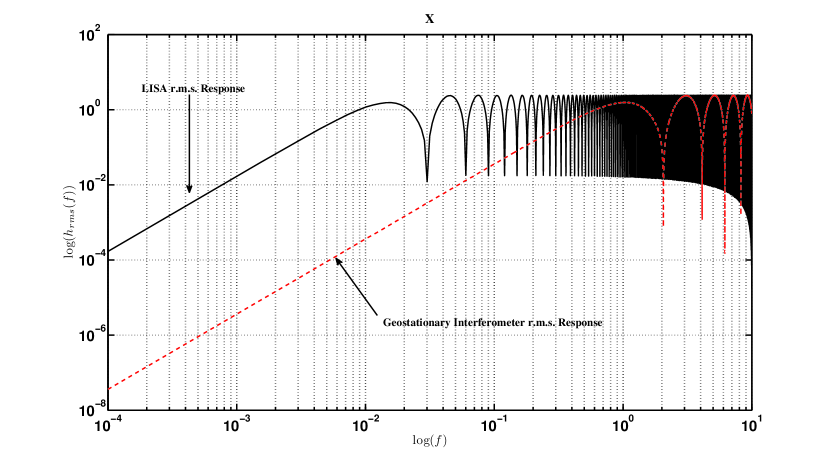
Figure 2: Root-Mean-Square response of the $X$ TDI combination for a geostationary interferometer. For completeness we have included also that for the interplanetary LISA mission, whose armlength is of $5\ \times 10^{6}$ km. The r.m.s. has been calculated by assuming an ensemble of sinusoidal signals uniformly distributed on the celestial sphere and randomly polarized.

In Figure 3 we then plot the sensitivities of the TDI combination $X$ for the various on-board hardware configurations discussed above. The characteristic behavior of the r.m.s. responses in Figure 2 folds into the plots presented here. At high-frequencies ($f\geq 0.05$ Hz) the sensitivities of the GEO1 and GEO2 configurations are significantly better than that of the LISA mission, while that of the GEO3 configuration shows a sensitivity marginally better than that of LISA only for frequencies $f\geq 0.5$ Hz. At lower frequencies instead, the LISA’s longer armlength results into a sensitivity better than those of the GEOGRAWI configurations we considered.

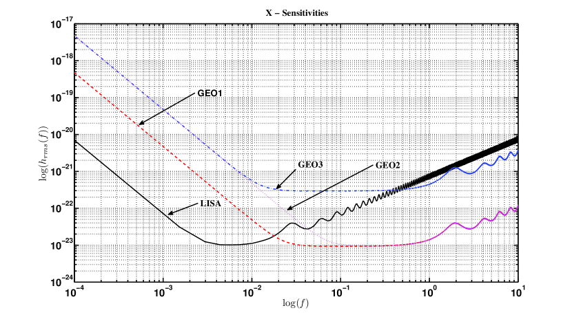
Figure 3: Sensitivity of the $X$ combination of a geostationary interferometer. Its noise performance is characterized by the noise spectra shown in Table (1) associated to the three different onboard subsystems configurations discussed. See text for more details.

Although the sensitivities at lower frequencies of any of the geostationary interferometers we considered are penalized by their shorter armlength or worse GRS noise, they can still provide a wealth of information about several astrophysical sources LISA was expected to detect and study. In the following section we turn to the science that a GEOGRAWI detector will be able to deliver.

3 Science with GEOGRAWI

In the previous section we have seen that a GEOGRAWI can operate in the $10^{-4}-10$ Hz frequency band, and it could be more sensitive than LISA (configuration (I,II) discussed in section 2) by a factor as large as $70$ in the frequency region above $20$ mHz. As a consequence of this result, it is natural to presume that a geostationary detector will be able to observe massive and super-massive Black Holes (SMBHs) and stellar-mass binary systems in the region of the frequency band where it achieves its best sensitivity. In the next subsections we focus our attention on SMBHs, as the sensitivity plots presented in Section 2 already imply the detectability of several binary systems present in our own galaxy (the so called “calibrators”) [7], and other sources emitting in the higher region of the accessible frequency band.

3.1 Detecting Supermassive Black Holes with GEOGRAWI

A significant amount of GW energy can be released during the three evolutionary phases (namely inspiral, merger and ring-down) of coalescing binaries containing SMBHs (BSMBH). To assess how well and how often a geostationary interferometer could detect SMBHs during these three phases, one should calculate the maximum redshift, for a given signal-to-noise ratio (SNR), at which these systems could be detectable.

To perform the calculations above one needs to know the waveforms. For the inspiral and ringdown phases there are well known analytical solutions [see, e.g., 29], which provide reliable results. For the merging phase, however, one needs to rely on fully numerical solutions of Einstein’s equations [30, 31, 32, 33, 34].

In recent years, it has been shown in the literature [see, e.g., 36] that there exist some reliable analytic approximations of the numerically derived waveforms valid under the assumption of two non-spinning black-holes.

In order to calculate the maximum redshift we consider the formula for the SNR based on the well known matched filtering technique (see, for example, Flanagan and Hughes [29]). The matched-filtering expression for the averaged squared SNR, in terms of the energy spectrum of the gravitational waves $dE/df$, is equal to [29]

$$\langle SNR^{2}\rangle=\frac{2(1+z)^{2}}{5\pi^{2}D_{L}(z)^{2}}\,\int_{0}^{\infty}df\,\frac{1}{f^{2}S_{h}(f)}\,\frac{dE}{df}[(1+z)f]\ ,$$ (4)

where $z$ is the cosmological redshift of the source, $D_{L}$ is the corresponding luminosity distance and $S_{h}(f)$ is the spectral density of the strain noise of the GW detector. On the left-hand-side of Eq. (4) the angle-brackets denote an ensemble average over sources uniformly distributed over the celestial sphere and polarization states.

Once the energy spectrum of the GWs (or its corresponding waveform) is given, Eq. (4) allows us to infer, for a given signal-to-noise ratio and a specific GEOGRAWI configuration, the maximum redshift at which a source can be detected, and then to estimate the SMBHs observable event rate.

It is worth noting that, although introduced many years before the first fully numerical relativity calculations of BBH mergers were available, the waveform proposed by Flanagan & Hughes [29] gives results that are within an order of magnitude of those derived numerically. Numerical relativity in fact showed that their white spectrum approximation for characterizing the merging phase resulted into an overestimated emitted GW energy [see, e.g., 37].

In the next subsections we separately consider the three different phases of the coalescing BSMBHs mentioned above. For the inspiraling and the ringdown phases we adopt the energy spectrum presented by Flanagan & Hughes [29]. For the merging phase we adopt instead the waveform by Ajith et al. [36], which captures in analytic form the features of the waveforms derived numerically for two non-spinning black holes. Some of our calculations are also based on the analysis recently done by Filloux et al. [38, 39] on the formation and evolution of SMBHs.

3.1.1 Detecting SMBH in the Ringdown phase

In the present study the SMBHs are formed as a result of the merging of two other SMBHs, which for simplicity have been assumed of equal masses. The SMBH so formed goes through the process of “ringdown”, and the resulting characteristic wave it emits is a damped sinusoid

$$h(t)\propto e^{-t/\tau}\cos(2\pi f_{rd}t)\ ,$$ (5)

where $\tau$ is the characteristic ringdown damping time and $f_{rd}$ is the frequency of the radiated signal. Following, e.g., Ref. [29], the energy spectrum is equal to

$$\frac{dE}{df}\simeq\frac{1}{8}{\cal A}^{2}QM^{2}f_{rd}\,\,\delta(f-f_{rd}),$$ (6)

where $M$ is the SMBH mass, ${\cal A}$ is a dimensionless coefficient that describes the magnitude of the perturbation when the ringdown begins and $Q$ is the quality factor of the mode.

Following Ref. [40], $f_{rd}$ and $Q$ can be related to the spin parameter $a$ and to the mass $M$ in the following way

$${f_{rd}}\simeq\left[1-0.63(1-a)^{3/10}\right]\ \frac{1}{2\pi M},$$ (7)

$$Q=\pi\tau f_{rd}\simeq 2\,(1-a)^{-9/20}\ .$$ (8)

The energy associated with the ringdown process can be written as

$$E_{\rm rd}\simeq\frac{1}{8}{\cal A}^{2}M^{2}f_{rd}Q,$$ (9)

which we will take to be a fraction, $\varepsilon_{rd}$, of the total mass $M$ of the black-hole. Although it has been argued in the literature that $\varepsilon_{rd}$ could very well be as large as a few percents (see Ref. [29] for an interesting discussion on this issue), here we will consider only two different (conservative) values for it, namely: $\varepsilon_{rd}=1\ \%$ and $\varepsilon_{rd}=0.1\ \%$.

Finally, from the above equations, the SNR (Eq. 4) can be rewritten in the following form

$$\langle SNR^{2}\rangle=\frac{8}{5}\,\frac{\varepsilon_{rd}}{D_{L}(z)^{2}F(a)^{2}}\frac{(1+z)^{3}M^{3}}{S_{h}[f_{rd}/(1+z)]},$$ (10)

where $F(a)=1-0.63(1-a)^{3/10}$.

With the expression (10) in hand we can calculate the redshift, $z_{max}$, below which a given SMBH of mass $M$ can be detected with a specified SNR, spin parameter $a$ and energy fraction $\varepsilon_{rd}$.

Since the luminosity distance depends on the cosmological parameters, in what follows we will assume a $\Lambda$CDM flat cosmology with the Hubble parameter $H_{0}=70\,{\rm km}\,{\rm s}^{-1}\,{\rm Mpc}^{-1}$, the total matter density parameter $\Omega_{m}=0.3$ and the cosmological constant density parameter $\Omega_{\Lambda}=0.70$.

In Figure 4 we plot $z_{max}$ as a function of the mass of the SMBH by taking ${\rm SNR}=10$ for the three GEOGRAWI configurations discussed in Section 2. Also shown for comparison are the results for LISA with (LISA CN) and without (LISA) the confusion noise (CN) contribution. Since $z_{max}$ mildly depends on the spin parameter $a$, we have fixed its value to $0.5$. On the other hand, since $z_{max}$ is very sensitive to the percentage of radiated energy, we have analyzed the following two possible values for $\varepsilon_{rd}$: $0.01$ and $0.001$.

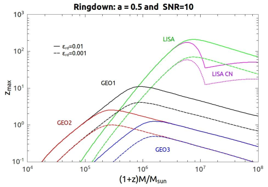
Figure 4: $z_{max}$ as a function of the SMBH mass M for $SNR=10$, $a=0.5$ and $\varepsilon_{rd}$ = 0.01 and 0.001, for the three GEOGRAWI configurations. Also shown for comparison are the results for LISA with (LISA CN) and without (LISA) the confusion noise contribution.

Although LISA can observe these signals at much larger redshifts than any GEOGRAWI configuration discussed in this article, the GEO1 configuration certainly represents an interesting alternative to LISA by being able to observe SMBHs at redshifts as high as $z=10$ when $\varepsilon_{rd}=0.01$.

From the above results we can now estimate the event rates of these systems for the different GEOGRAWI configurations. To perform this calculation we model the formation of SMBHs by relying on a recent study by Filloux et al. (see [38] and references therein), where the coalescence history of SMBHs is derived from cosmological simulations. Filloux et al. were able to derive the coalescence rate per unit volume and mass intervals as a function of the resulting BH mass and redshift (see Fig. 3 of [38]), $\Psi(M,z)$. With $\Psi(M,z)$ we can write the differential coalescence rate at the detector frame in the following way

$$dR_{obs}(M,z)=\frac{\Psi(M,z)}{1+z}dM\frac{dV}{dz}dz\ ,$$ (11)

where the factor $(1+z)$ takes into account the time dilation.

For additional discussions, concerning the coalescence rate related to this study and the corresponding cosmological simulations, besides Ref. [38] we refer the reader to Ref. [39] and B.

Note that the above equation depends on the co-moving volume element $dV$ which, for a flat cosmology, is equal to

$$dV=4\pi\left(\frac{c}{H_{0}}\right)\frac{r^{2}(z)dz}{\sqrt{\Omega_{\Lambda}+\Omega_{m}(1+z)^{3}}}$$ (12)

and $r(z)$ is the co-moving distance

$$r(z)=\frac{c}{H_{0}}\int_{0}^{z}\frac{dz^{\prime}}{\sqrt{\Omega_{\Lambda}+\Omega_{m}(1+z^{\prime})^{3}}}.$$ (13)

With $z_{max}(M)$ we can now integrate Eq. (11) in the $M$ and $z$ variables to estimate the event rate for each GEOGRAWI configuration as a function of the SNR, $a$ and $\varepsilon_{rd}$.

In Table II we show our estimated ringdown observation rates for GEOGRAWI and, for comparison, also those for LISA. It can be noticed that, for $\varepsilon_{rd}=0.01$, the event rates for GEO1 are comparable to those for LISA. This can be better understood with the aid of Fig.5, which shows the logarithmic differential ringdown observation rate as a function of frequency, together with the differential ringdown rate for comparison (see B for details.)

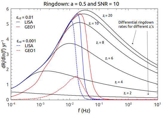
Figure 5: Differential ringdown observation rate as a function of frequency for the GEOGRAWI configuration 1 (GEO1) and for LISA. Also plotted, the differential ringdown production rate for different initial redshifts (notice that not all of it is seen neither by LISA nor GEO1); see B for details.

Note that when $\varepsilon_{rd}=0.01$ the curve of the differential ringdown observation rate of GEO1 extends at higher frequencies more than the LISA curve. In this region of its accessible frequency band GEO1 can detect ringdown gravitational waves emitted by systems of smaller masses. Since these observed systems are larger in number than the more massive SMBHs, we can see why GEO1 has a ringdown observation rate comparable to that of LISA. On the other hand, as it will be shown in section 3.1.3, these same systems will be observed by LISA with a SNR larger than that achievable by GEO1 during the inspiraling phase.

As shown in B, the model by Filloux et al. [38] for the current value of the coalescence rate amounts to $\simeq$ 43 yr^-1. This implies that, depending on the values of $\varepsilon_{rd}$ and $a$, GEO1 can detect a large fraction of ringdown SMBHs.

Table 2: The ringdown observation rates for LISA, GEO1, GEO2 and GEO3 with a SNR = 10 and for different values of $\varepsilon_{rd}$ and $a$.

Antenna		$a$		$\varepsilon_{rd}$		R(yr-1)
LISA CN		0		0.001		16.8
LISA CN		0.5		0.001		15.7
LISA CN		0.95		0.001		14.1
LISA CN		0		0.01		19.8
LISA CN		0.5		0.01		18.5
LISA CN		0.95		0.01		16.7
GEO1		0		0.001		2.41
GEO1		0.5		0.001		3.27
GEO1		0.95		0.001		5.29
GEO1		0		0.01		16.8
GEO1		0.5		0.01		18.3
GEO1		0.95		0.01		19.0
GEO2		0		0.001		0.049
GEO2		0.5		0.001		0.066
GEO2		0.95		0.001		0.10
GEO2		0		0.01		0.58
GEO2		0.5		0.01		0.82
GEO2		0.95		0.01		1.35
GEO3		0		0.001		0.008
GEO3		0.5		0.001		0.011
GEO3		0.95		0.001		0.018
GEO3		0		0.01		0.098
GEO3		0.5		0.01		0.13
GEO3		0.95		0.01		0.22

3.1.2 Detecting SMBH in the Merger phase

The merger phase can be related to the Fourier frequency interval associated to the merger (lower) frequency $f_{m}$ all the way to the ring-down frequency $f_{rd}$. During this evolutionary phase a significant amount of GW energy, comparable to that emitted during the ring-down phase, is radiated.

One of the main issues regarding the characterization of the merger phase is the determination of the frequency $f_{m}$. We do not address this issue here, and refer the reader to Ajith et al. [36], where it is shown that $f_{m}\simeq 0.04/M$ for equal mass BBH systems. Also in [36] it is shown that there exist a reliable analytic approximation for the merging-phase waveforms derived numerically. The resulting expression for the radiated energy spectrum is equal to

$$\frac{dE}{df}=\frac{1}{3}\pi^{2/3}\mu M^{2/3}\frac{f^{2/3}}{f_{m}}$$ (14)

which is valid for two non-spinning and equal mass black-holes.

Finally, substituting the above equation into equation (4) we get

$$\langle SNR^{2}\rangle=\frac{[(1+z)M]^{5/3}}{30\pi^{4/3}f_{m}D_{L}(z)^{2}}\,\int_{f_{min}/(1+z)}^{f_{m}/(1+z)}\,\frac{df}{f^{4/3}S_{h}(f)}.$$ (15)

Following the same prescription as for the ring-down case, we can then calculate the redshift, $z_{max}$, below which a given SMBH of mass $M$ can be detected with a given SNR. In Figure 6 we plot $z_{max}$, for the three different GEOGRAWI configurations, as a function of the mass $M$ of the SMBH system. As before we have included the results valid for LISA and LISA CN. Also in this case the GEO1 configuration represents an interesting alternative to LISA as merging SMBHs could be seen at redshifts as high as $z=10$.

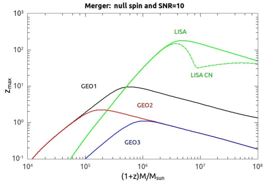
Figure 6: $z_{max}$ as a function of the SMBH mass M for $SNR=10$, and null spin, for the different GEOGRAWI configurations. Included for comparison are the results for LISA and LISA CN.

For sake of curiosity, we compared our results against those corresponding to a “white” spectrum [29]. We found that the two would agree quite well by assuming a white spectrum corresponding to an energy emission efficiency of about $1\%$ (i.e. $1\%$ of the total mass $M$ of the BBHs is converted to gravitational radiation).

3.1.3 Detecting SMBH in the inspiral phase

In this section we finally analyze the inspiraling phase of a binary system containing SMBH. In this case the signals frequency components will fall into the region of the band where $f<f_{m}$, which is accessible to all the GEOGRAWI configurations considered here.

The energy spectrum for the inspiraling phase is given by the well known formula [1]

$$\frac{dE}{df}=\frac{1}{3}\pi^{2/3}\mu M^{2/3}f^{-1/3}\$$ (16)

and, for the particular case of binary systems whose components have equal mass, the SNR becomes equal to

$$\langle SNR^{2}\rangle=\frac{[(1+z)M]^{5/3}}{30\pi^{4/3}D_{L}(z)^{2}}\,\int_{f_{min}/(1+z)}^{f_{m}/(1+z)}\,\frac{df}{f^{7/3}S_{h}(f)}.$$ (17)

Note that now, in order to obtain $z_{max}$ as a function of $M$, we had to treat the $SNR$ and $f_{min}$ as free parameters. As before, we take the $SNR=10$. The value of $f_{min}$ is chosen in such a way that the signal is integrated (observed) over the last year of inspiraling. For binary systems whose components have equal masses it is easy to show that $f_{min}$ is given by the following expression

$$f_{min}(T)=\left\{f_{m}^{-8/3}+\frac{64}{5}\pi^{8/3}[M(1+z)]^{5/3}T\right\}^{-3/8},$$ (18)

where $T$ is the time before merging. In Figure 7 we plot $z_{max}$ as a function of the mass of the system of SMBHs for ${\rm SNR}=10$ and for one year of observation.

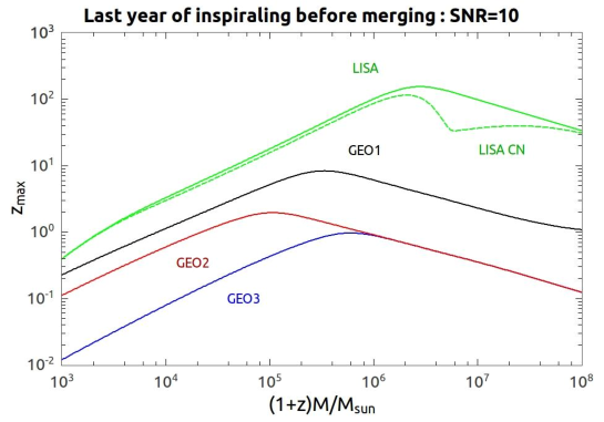
Figure 7: $z_{max}$ as a function of the SMBH mass M for $SNR=10$ for the different GEOGRAWI configurations. Also shown for comparison are the curves corresponding to LISA and LISA CN.

Although Fig. (7) shows that, at an SNR=10, the maximum redshift achievable by LISA is consistently larger than that for GEO1, also indicates that the maximum redshift at which the coalescence phase can be observed by GEO1 is equal to about 5.

In summary, LISA can reach a larger redshift as compared to any GEOGRAWI configuration independently of the SMBH masses.

4 Conclusions

The main goal of this article was to analyze the performance and some scientific capabilities of a geostationary gravitational wave interferometer. We have done so by estimating its sensitivities to gravitational radiation when operated under three different onboard subsystem configurations, and analyzed the kind of gravitational wave sources it will be able to detect and study in the sub-Hertz band. We found our proposed Earth-orbiting detector less sensitive than the Laser Interferometer Space Antenna mission by about a factor of seventy in the lower part of its accessible frequency band ($10^{-4}-2\times 10^{-2}$ Hz). On the other hand, in the higher part of the band ($2\times 10^{-2}-10$ Hz), it was shown that GEOGRAWI has observational capabilities that are complementary to those of the LISA mission. In relation to this point, we emphasized that our assumed noise performance in the high-frequency region of the accessible band requires additional instrumental capabilities over those baselined for the LISA mission. Although current experimental evidence [22, 23, 24] indicates that they will be available by the time such a mission will be considered, a more in-depth analysis of these challenges is beyond the scope of this paper.

In the case of binary systems containing SMBHs, our analysis has shown that the GEO1 interferometer could observe a great number of events per year. This is direct consequence of its good sensitivity in the frequency region ($2\times 10^{-2}-10$ Hz), where lighter (and larger in number) black-holes radiate in the merger and ring-down phases. Consistently we have also shown that these same systems will be detectable by LISA with a SNR larger than that achievable by GEO1 during the inspiraling phase (see Fig. 7).

Since most of the SNR from the coalescence phase of a binary system containing SMBHs is achieved after about a week of integration time before coalescence, because GEOGRAWI will make most of its observations in the high-part of its accessible frequency band, and because during a time period of one week the amplitude modulation of the GEOGRAWI response will result into a frequency modulation of the observed GW signal that depends on the source location in the sky, one can argue that GEOGRAWI should achieve very good accuracies in the reconstructed GW source parameters of SMBH with masses that are in the range $10^{4}-10^{6}\ M_{\odot}$. It is worth noting that McWilliams [11, 41] has performed such an analysis for the GADFLI mission concept (which is similar to GEOGRAWI). He showed that the precision in the estimation of the parameters achievable by GADFLI (which is analogous to our GEO1 configuration) is somewhat better than that for LISA. Although these results imply that GEO1 should achieve comparable accuracies in estimating the parameters characterizing SMBHB, it is our intention to quantitatively study this problem in a forthcoming article.

Since the high-part of the accessible frequency where GEOGRAWI achieves its best sensitivity is at around $1$ Hz, we will investigate also its ability to perform low-latency searches of burst events. Mainly due to its capability of continuously transmitting real-time data to the ground (by being geostationary), it should be able to trigger simultaneous searches for electromagnetic counter-parts.

Appendix A Noise analysis

In this Appendix we provide an analysis of the noise sources affecting the heterodyne measurements performed by the geostationary GW interferometer GEO1. Since some of its onboard instrumentation is similar to that of the LISA mission, it imposes the most stringent noise-performance requirements on the subsystems affecting the one-way heterodyne measurements. Furthermore, as it will be discussed below, the noise performance in the high-frequency region of the accessible band requires additional instrumental capabilities over those baselined for the LISA mission. Although current experimental evidence [42, 43, 44, 45, 22, 23, 24] induces us to believe that they will be available by the time such a mission will be further analyzed, it is clear that these potential challenges are well beyond the scope of this paper.

Our analysis will also rely on two LISA study documents as guiding references [7, 21]. There it was shown that there exist two main categories of sensitivity-limiting noise sources:

1. Acceleration noises

2. Optical-Path noises

The acceleration noises are due to residual forces acting on the proof-masses of the Gravitational Reduction System (GRS), and result into Doppler fluctuations into the heterodyne measurements. Their magnitudes are most prominent in the low-part of the accessible frequency band ($10^{-4}-10^{-2}$ Hz) and depend on the (i) adopted GRS design, (ii) the spacecraft design, and (iii) the mission trajectory and space environment within which the spacecraft will be operating. For these reasons the classification of the acceleration noises is a multi-parameters problem and a very challenging one. In the case of the LISA mission this has already been studied extensively and it will be finalized through the LISA Pathfinder experiment [25, 26]. This is a ESA mission aimed at testing the noise modeling, classification, and performance of the LISA GRS system.

The LISA GRS was envisioned to have two cubic proof-masses onboard each spacecraft and whose positions relative to the spacecraft were measured with electrostatic (capacitative) readouts that were part of their caging systems. In recent years, however, it has been argued that a single, spherical proof-mass design (whose position relative to its enclosing cage is measured optically) could be used instead, providing significant simplifications of the GRS and of the optical bench where the heterodyne measurements are performed [46].

Although a single, spherical proof-mass GRS implementation might result into a better noise performance than that with two cubic masses [46], in our analysis we will assume GEO1 to rely on a spherical GRS design whose performance is similar to that of the LISA GRS, i.e. with a square-root of the acceleration spectral density equal to a value of $3\ \times 10^{-15}\ {\rm m/s}\ {\rm Hz}^{-1/2}$ over the accessible frequency band. In ultimate analysis it will be the LISA Pathfinder experiment that will show us whether the types and magnitudes of the noise sources affecting the GRS performance are what we expect them to be.

The primary noise sources within the second category, i.e. Optical-path noises, are much easier to identify and are most prominent in the higher part of the accessible frequency band. They can be summarized as [7, 21]

• Shot-noise at the photo-detectors,

• Residual laser phase noise in the TDI observables,

• Laser beam-pointing fluctuations,

• Phase-meter noise,

• Master clock noise,

• Scattered light effects.

The Shot-Noise is a fundamental noise limitation to the sensitivity of a laser interferometer GW detector in the high-part of its accessible frequency band. It affects the one-way Doppler measurements right at the photo-detector where two laser beams are made to interfere, and it leads to the following spectral density of relative frequency (Doppler) fluctuations [7]

$$S_{\rm shot}(f)=\frac{hf^{2}}{\nu_{0}\ P_{\rm avail}}\ .$$ (19)

In Eq. (19) $h$ is the Planck constant, $\nu_{0}\equiv 3.0\times 10^{14}{\rm Hz}$ is the nominal laser frequency, $f$ is the Fourier frequency, and $P_{\rm avail}$ is the effective power available at the receiving photodetector. By assuming the same optics, optical telescope size, laser power, and photodetector quantum efficiency as those of LISA, from Eq. (19) we conclude that the amplitude of the relative frequency fluctuations due to shot noise affecting the GEO1 interferometer scale down linearly with the interferometer armlength.

The Residual laser phase noise represents the “left-over” of the laser noise in the TDI observables after the TDI algorithm is applied to the one-way Doppler measurements by properly time-shifting and linearly combining them. It is primarily due to the finiteness in the accuracy by which the armlengths are known, and is proportional to the amplitude of the laser frequency fluctuations. The relationship between the magnitude of the spectrum of the residual laser frequency fluctuations, $S_{\Delta C}(f)$, and the armlength accuracies, $\delta L_{i}\ ,i=1,2$, is given in [47] for the unequal-arm Michelson interferometer TDI combination and has the following form

$$S_{\Delta C}(f) = 64\pi^{2}f^{2}S_{C}(f)\left\{\delta L_{1}^{2}\sin^{2}(2\pi fL_{2})+\delta L_{2}^{2}\sin^{2}(2\pi fL_{1})\right.$$ (20)

$$- \left.\delta L_{1}\delta L_{2}[\sin^{2}(2\pi fL_{1})+\sin^{2}(2\pi fL_{2})-\sin^{2}(2\pi f(L_{2}-L_{1}))]\right\}\ .$$

In the long-wavelength limit it is easy to show from the above equation that the amplitude of the residual laser frequency fluctuations scale linearly with the armlength of the interferometer (see Eq. (3.18) of [47]). On the other hand, this scaling no longer exists at higher-frequencies and, in order to maintain this noise source negligible in the GEO1 noise budget, a higher level of accuracy in the knowledge of the armlengths is required. Since the GEO1 configuration will have a shot noise amplitude smaller than that of LISA by about a factor of $70$, by measuring the GEO1 armlength with an accuracy that is seventy times better than that of LISA we will make this noise source negligible in the GEO1 TDI combination $X$. Given that the required LISA armlength accuracy for $X$ has been estimated to be equal to about $30$ meters [47], we conclude that the armlength accuracy needed for GEO1 should be of about $40$ centimeters. Such a level of laser ranging accuracy has already been demonstrated experimentally [42] at a much lower receiving laser power. This means that, in the case of the GEO1 mission, the achievable armlength accuracy will be smaller than $40$ cm, further reducing the GEO1 residual laser frequency noise.

The Laser beam-pointing fluctuations are due to distortions in the transmitted laser beam wavefront that appear at the receiving spacecraft as additional frequency fluctuations generated by small pointing fluctuations from the transmitting spacecraft. In the case of the LISA mission, whose pointing fluctuations specifications were required not to be greater than $6\ {\rm nrad}\ {\rm Hz}^{-1/2}$, it was shown [43] that a way for substantially reducing pointing-induced frequency fluctuations was to rely on the light received from the far spacecraft to sense the orientation of the receiving spacecraft. An ingenious way for doing so [43] is by sampling some of the incoming light on a CCD array. By detecting the position of the beam on the CCD it is then possible to deduce the alignment of the spacecraft and implement it by proper control signals. This measurement is shot-noise limited and, in the case of the LISA mission, it was proposed to implement it by extracting $10$ percent of the power of the incoming laser light. This resulted into a pointing noise of about $0.5\ {\rm nrad}\ {\rm Hz}^{-1/2}$, more than a factor of $10$ better than that specified for LISA. Since the shot-noise level associated with this pointing measurement technique scales down linearly with the armlength (by being inversely proportional to the square-root of the received laser power) we conclude that the pointing shot-noise limit for GEO1 will scale down linearly with the armlength from the level estimated for LISA.

The Phase-meter is the subsystem that measures the difference between the phase of the incoming laser beam and that from the local laser, and in the process it introduces an additional phase noise in the one-way Doppler measurements. Although the noise it generates does not scale with the armlength, it does depend on the magnitude of the relative frequency offset between the transmitted and received frequencies of the two interfering laser beams [44]. As an example, it has been shown that the frequency stability of the phase-meter to be flown on the LISA Pathfinder mission (which has an heterodyne frequency range of about a few kHz) will be several orders of magnitude better than that of the phase-meter for the LISA mission [44, 45]. It is for this reason that, in order to compensate for the Sun and the Moon gravitational perturbations on each spacecraft and maintain orbital stability and small inter-spacecraft relative velocities, each spacecraft will implement “station-keeping” [20, 48]. Since this operation will need to be performed about once per week [49] in order to maintain the spacecraft relative velocities smaller than about a few decimeters per second, it will not disrupt significantly the science data acquisition. As an additional note, GEO1 will also rely on molecular iodine laser frequency stabilization, which has been shown to provide laser frequency stability superior to that achievable by optical cavity stabilization and a laser frequency accuracy at the level of $1$ to $2$ kHz [22].

The Master clock noise affects the LISA measurements because it is used for removing the large Doppler beat-notes (as large as $20$ MHz) affecting the Doppler measurements. Since GEO1 will not be subject to large orbital perturbations as those affecting LISA and it will rely on station-keeping in order to maintain a “stationary” configuration, the noise due to the onboard master clock for performing the heterodyne measurements will be negligible as it is proportional to the magnitude of the beat note at the photodetector [50]. This will result into a significant simplification of the designs of the phase-meter and transmitting modules as modulations of the transmitting and receiving beam (for implementing the clock-noise cancellation scheme) will not be needed.

Scattered Light effects are due to spurious light signals generated from the interaction of the received main laser beam with the optical telescope, beam-splitter, and other optical components of the optical bench the beam interacts with before being made to interfere with the light of the local laser. Although this noise source for quite sometimes has been thought to be unavoidable, in recent years new developments in laser metrology have indicated that scattered light noise can be suppressed to sub-picometer levels in the frequency band of interest to space-based GW interferometers. In one such laser metrology technique, called “Digital Interferometry” (DI) [23, 24], laser light is phase modulated with a pseudo-random noise (PRN) code that time stamps the light, allowing isolation of individual propagation paths based on their times of flight through the system. After detection, the PRN phase shift is removed by decoding with an appropriately delayed copy of the code. By matching the decoding delay to the propagation delay the signal is coherently recovered, allowing phase measurements to extract displacement information at resolutions much smaller than the laser wavelength. This matched-delay filtering of DI allows isolation of reflections from an object at a particular distance, such as the optical components giving origin to the scattered light noise.

In summary, the magnitude of the relative frequency fluctuations due to the shot-noise and the laser beam-pointing fluctuations scale linearly with the armlength, as it follows from the considerations leading to equation (4.4) at page 82 of [7], and sections 3 at page 1576 of [43] respectively. Although the frequency fluctuations due to the residual laser phase noise, the scattered-light noise, and the phase-meter noise do not follow a similar scaling, we have shown that they can be made negligible within the GEO1 noise budget. This is because of a demonstrated better armlength accuracy [42], of digital interferometry as it suppresses scattered light effects, and adoption of a simpler phase-meter design [44] that takes advantage of much smaller “beat-note” frequencies among the lasers. The latter is made possible through a combination of laser iodine stabilization [22] together with spacecraft station-keeping maneuvers [20].

Appendix B Coalescence rate

In this Appendix we discuss the differential coalescence rate per logarithm frequency interval as this can be related to the differential event rate associated, for example, with the ring-down phase shown in Fig. 5. For a more detailed analysis regarding the coalescence rate and the corresponding cosmological simulations, we refer the reader to Refs. [38] and [39] respectively.

The differential coalescence rate is obtained from an appropriate combination of Eqs. (11) and (7) and an integration in a given redshift interval, namely $0<z<z_{initial}$, where $z_{initial}$ refers to a value selected at the beginning of the simulation.

Fig. 8 shows the differential coalescence rate per logarithmic frequency interval as a function of the frequency and for different intervals of integration in the redshift. We have not included curves corresponding to values of the redshift higher than $20$ because they all “saturate” to the curve corresponding to this value of $z_{initial}$.

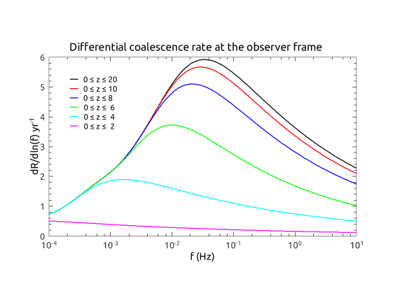
Figure 8: Differential coalescence rate as a function of the Fourier frequency and for different interval of integration in redshift.

Another interesting information concerning the study by Filloux et al. [38] refers to the coalescence rate at the observer frame, which can be obtained by integrating the differential coalescence rate. After performing such an integration we find a coalescence rate of $\sim$ 43 yr^-1 (associated with the ring-down phase), which should be regarded as the maximum event rate a given gravitational wave antenna might detect. Our study has actually shown that LISA and GEO1 should be able to detect a large fraction of this rate.

Implicit in the integration just mentioned, there is an integration in the redshift interval $0<z<z_{initial}$, where $z_{initial}$ was taken to be equal to $60$ in the present study. In practice, however, there is a saturation around $z\sim 12$, as can be seen in Fig. 9, where the cumulative event rate as a function of $z_{initial}$ is plotted and tabulated. Note that half of the coalescence rate comes from events occurring at $z>5$.

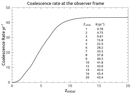
Figure 9: Coalescence rate as a function of $z_{initial}$. Note how this function starts to plateau at $z_{initial}\approx 12$.

References

- Thorne [1987] Thorne, K. S., 1987. In: Three Hundred Years of Gravitation, 330-458, Eds. Hawking, S. W., & Israel, W., (Cambridge University Press, New York)
- LIGO [2012] http://www.ligo.caltech.edu/ .
- VIRGO [2012] http://www.virgo.infn.it/ .
- GEO [2012] http://www.geo600.uni-hannover.de/ .
- TAMA [2012] http://tamago.mtk.nao.ac.jp/ .
- Detweiler [1979] Detweiler, S., 1979, Ap. J., 234, 1100-1104.
- Bender et al. [1998] P. Bender, K. Danzmann, & the LISA Study Team, 1998, Laser Interferometer Space Antenna for the Detection of Gravitational Waves, Pre-Phase A Report, MPQ233 (Max-Planck- Institüt für Quantenoptik, Garching, Germany.
- Ni [2002] Ni, W. T., 2002, Int. J. Mod. Phys. D, 11 (7), 947.
- Seto et al. [2001] Seto, N., Kawamura, S., & Nakamura, T., 2001, Phys. Rev. Lett, 87, 221103.
- Hiscock & Hellings [1997] Hiscock, B., Hellings, R. W., 1997, Bull. Am. Astron. Soc., 29, 1312.
- Physics of the Cosmos [2012] http://pcos.gsfc.nasa.gov/studies/gravitational-wave-mission.php/ .
- NRC Report [2010] NRC 2010, http:// www.nap.edu/catalog/12951.html
- NASA Solicitation [2011] NASA solicitation # NNH11ZDA019L titled: Concepts for the NASA Gravitational-Wave Mission. Document available at: http://nspires.nasaprs.com/external/ .
- Tinto et al. [2011] Tinto, M., de Araujo, J. C. N., Aguiar, O. D., & M.E.S. Alves, 2011, A Geostationary Gravitational Wave Interferometer (GEOGRAWI) (http://arxiv.org/pdf/1111.2576.pdf).
- McWilliams [2011] McWilliams, S. T., 2011, Geostationary Antenna for Disturbance-Free Laser Interferometry (GADFLI) (http://arxiv.org/PS_cache/arxiv/pdf/1111/1111.3708v1.pdf).
- Tinto & Alves [2010] Tinto, M., & Alves, M. E. S., 2010, Phys. Rev. D, 82, 122003.
- Edlund et al. [2005] Edlund, J. A., Tinto, M., Królak, A., & Nelemans, G., 2005, Classic. Quantum Grav., 22, S913-S926.
- Tinto & Dhurandhar [2005] Tinto, M., & Dhurandhar, S. V., 2005, Living Rev. Relativity, 8, 4. http://www.livingreviews.org/lrr-2005-4
- Hellings et al. [2011] Hellings, R., Larson, S. L., Jensen, S., Fish, C., Benacquista, M., Cornish, N., & Lang, R., A LOW-COST, HIGH-PERFORMANCE SPACE GRAVITATIONAL ASTRONOMY MISSION (http://pcos.gsfc.nasa.gov/studies/rfi/GWRFI-0007-Hellings.pdf).
- Soop [1994] Soop, E. M., 1994,Handbook of Geostationary Orbits, Kluwer Academic Publishers (Dordrecht, The Netherlands).
- LISA Study [2011] “LISA: Unveiling a hidden Universe”, ESA publication # ESA/SRE(2011)3 (February 2011). Also available at: http://sci.esa.int/science-e/www/object/index.cfm?fobjectid=48364
- Leonhardt & Camp [2006] Leonhardt, V., & Camp, J.B., 2006, APPLIED OPTICS, 45, 4142.
- Shaddock [2007] Shaddock, D. A., 2007, Opt. Lett., 32, 3355.
- Wuchenich et al. [2011] Wuchenich, D. M. R., Lam, T. T.-Y., Chow, J. H., McClelland, D. E., & Shaddock, D. A., 2011, Opt. Lett., 36, 672.
- Antonucci et al. [2011] Antonucci, F., et al, 2011, Class. Quantum Grav., 28 094001.
- Antonucci et al. [2011] Antonucci, F., et al, 2011, Class. Quantum Grav., 28 094002.
- Armstrong et al. [1999] Armstrong, J. W., Estabrook, F. B., & M. Tinto, 1999, Ap. J., 527, 814.
- Estabrook et al. [2000] Estabrook, F. B., Tinto, M., & Armstrong, J. W., 2000, Phys. Rev. D, 62, 042002.
- Flanagan & Hughes [1998] Flanagan, E. E., & Hughes, S. A., 1998, Phys. Rev. D, 57, 4535.
- Pretorius [2005] Pretorius, F., 2005, Phys. Rev. Letters, 95, 121101.
- Baker et al [2006] Baker, J. G., Centrella, J. M,. Choi, D.-I., Koppitz, M. & van Meter, J. R., 2006, Phys. Rev. Letters, 96, 111102
- Campanelli et al [2006] Campanelli, M., Lousto, C. O., Marronetti, P. & Zlochower, Y., 2006, Phys. Rev. Letters, 96, 111101.
- McWilliams [2011] McWilliams, S. T., 2011, Class. Quantum Grav., 28, 134001
- Hinder [2010] Hinder, I., 2010, Class. Quantum Grav., 27, 114004
- Centrella et al [2010] Centrella, J. M., Baker, J. G., Kelly, B. J. & van Meter, J. R., 2010, Phys. Rev. Mod. Phys., 82, 3069.
- Ajith [2008] Ajith, P., Babak, S., Chen, Y., Hewitson, M., Krishnan, B., Sintes, A. M., Whelan, J. T., Brügmann, B., Diener, P., Dorband, N., Gonzalez, J., Hannam, M., Husa, S., Pollney, D., Rezzolla, L., Santamaría, L., Sperhake, U., & Thornburg, J., 2008, Phys. Rev. D, 77, 104017
- Baker [1989] Baker, J. G., McWilliams, S. T., van Meter, J. R., Centrella, J. M. Choi, D.-I., Kelly, B. J. & Koppitz, M., 2007, Phys.Rev. D 75, 124024.
- Filloux et al. [2011] Filloux, Ch., de Freitas Pacheco, J. A., Durier, F. & de Araujo, J. C. N., 2011, IJMPD, 20, 2399.
- Filloux et al. [2010] Filloux, Ch., Durier, F., de Freitas Pacheco, J. A. & Silk, J., 2010, IJMPD, 19, 1233.
- Echeverria [1989] Echeverria, F., 1989, Phys.Rev. D 40, 3194.
- [41] http://www.apc.univ-paris7.fr/FACe/en/content/elisango
- Esteban et al. [2011] Esteban, J. J., Garcia, A. F., Barke, S., Peinado, A. M., Cervantes, F. G., Bykov, I., Heinzel, G., & K. Danzmann, 2011, Opt. Express, 19, 15937.
- Robertson et al. [1997] Robertson, D. I., McNamara, P., Ward, H., & Hough, J., 1997, Class. Quantum Grav., 14, 1575.
- Wand [2007] Wand, V., 2007, Interferometry at low frequencies: optical phase measurement for LISA and LISA Pathfinder, Ph. D. thesis, University of Hannover, unpublished.
- Shaddock et al. [2006] Shaddock, D., Ware, B., Halverson, P., Spero, R. E., & Klipstein, B., 2006, Overview of the LISA Phasemeter, International LISA Symposium, eds. S.M. Merkowitz, & J.C. Livas, Springer (Berlin, Germnay, pp. 654-660).
- Sun et al. [2005] Sun, Ke-Xun, Allen, G., Buchman, S., DeBra, D., & Byer, R., 2005, Class. Quantum Grav., 22, S287 - S296.
- Tinto & Armstrong [1999] Tinto, M., & Armstrong, J. W., 1999, Phys. Rev. D, 59, 102003.
- Maral & Bousquet [2009] Maral, G., & Bousquet, M., 2009, Satellite Communications Systems, fifth edition, John Wiley & Sons, (Chichester, England, U.K.)
- Kamel et al. [1999] Kamel, A. A., Gelon, W., & Reckdahl, K., 1999. In proceedings of: AAS/AIAA Astrodynamics Specialist Conference, Girdwood, Alaska, August 16-18, AAS Paper No. AAS 99-388.
- Tinto et al. [2002] Tinto, M., Estabrook, F. B., & J.A. Armstrong, 2002, Phys. Rev. D, 65, 082003.