Are private schools better than public schools? Appraisal for Ireland by methods for observational studies

Abstract

In observational studies the assignment of units to treatments is not under control. Consequently, the estimation and comparison of treatment effects based on the empirical distribution of the responses can be biased since the units exposed to the various treatments could differ in important unknown pretreatment characteristics, which are related to the response. An important example studied in this article is the question of whether private schools offer better quality of education than public schools. In order to address this question, we use data collected in the year 2000 by OECD for the Programme for International Student Assessment (PISA). Focusing for illustration on scores in mathematics of 15-year-old pupils in Ireland, we find that the raw average score of pupils in private schools is higher than of pupils in public schools. However, application of a newly proposed method for observational studies suggests that the less able pupils tend to enroll in public schools, such that their lower scores are not necessarily an indication of bad quality of the public schools. Indeed, when comparing the average score in the two types of schools after adjusting for the enrollment effects, we find quite surprisingly that public schools perform better on average. This outcome is supported by the methods of instrumental variables and latent variables, commonly used by econometricians for analyzing and evaluating social programs.

Are private schools better than public schools? Appraisal for Ireland by methods for observational studies

TITL1Supported by the Israel Science Foundation Grant 1277/05.

and

1 Introduction

In observational studies the assignment of units to treatments often depends on latent variables that are related to the response variable even when conditioning on known covariates. Consequently, a direct comparison of the response distributions (given the model covariates) or moments of these distributions between treatment groups could be biased and result in wrong conclusions. An important example studied in this article is the question of whether private schools offer better quality of education than public schools. This question has important impact on educational policy and public finance [Hanushek (2002)]. It is known that pupils enrolling to the two types of schools differ in their family background and other characteristics related to their scholastic achievements, such that a raw comparison of the scores of pupils attending the two types of schools can be misleading. In an attempt to deal with this question, we use data collected in the year 2000 by OECD for the Programme for International Student Assessment (PISA). The purpose of this program is to study and compare the proficiency of pupils aged 15 from over more than 30 countries in mathematics, science and reading. In this article we focus on scores in mathematics in Ireland and estimate the difference in the average score between the two types of schools by adjusting for the quality of pupils enrolling to them and for the effects of known covariates.

We start by applying several existing methods for observational studies to the data, which are described in Section 3, and find, similarly to Vanderberghe and Robin (2004), that some of these methods produce estimates of different magnitude and sign. We attempt to resolve this conflict by developing and applying a new method for inference from observational data, which extends recent methodology for analyzing sample survey data. The method derives the sample distribution of the observed response under a given treatment (score in mathematics in a given type of school in our application) as a function of the distribution that would be obtained under a strongly ignorable assignment of subjects to treatments (assumptions $\operatorname{SI}(a)$, $\operatorname{SI}(b)$ in Section 3), and the assignment probability, which is allowed to depend on the response value. The use of this approach is established by showing that the sample distribution is identifiable under some general conditions. The goodness of fit of the sample distribution can be tested by standard test statistics since it refers to the observed data.

By fitting the sample distribution to the observed data, we can estimate the distribution under strongly ignorable assignment to treatments, and the assignment probabilities, which are then used for estimating population means or contrasts between them. Our approach permits also testing some of the assumptions underlying other methods for analyzing observational data, thus enabling us to understand better why different methods yield different answers in our application.

Section 2 describes the PISA data and defines the problem underlying this study more formally. Section 3 overviews some of the existing methods for observational studies and shows the results obtained when applying them to the PISA data for Ireland. We also consider “probability weighted” versions of the estimators, which account for unequal sample selection probabilities that are possibly related to the response and may thus bias the inference. Computation of these estimators yields very similar estimates to the estimates obtained under the standard methods. Section 4 presents the proposed approach and shows the results obtained when applying it to the PISA data. The main outcome of this analysis is that after controlling for the effect of the enrollment process, the public schools actually outperform the private schools in the average math score, suggesting better quality of education. Here also we extend the method to account for unequal selection probabilities and obtain similar estimates. Section 5 overviews the main theoretical properties of the new approach. The technical derivations are presented in Supplements C and D of the supplementary material [Pfeffermann and Landsman (2011)]. We conclude with a brief summary in Section 6.

2 Data used for application and formulation of the problem

2.1 Sampling design and response values

In order to compare the private and public schools, we use data collected in Ireland in the year 2000 by OECD for PISA.

Sampling design

PISA uses in most countries a stratified two-stage sampling design. The strata are defined by the size of the school, type of school and gender composition. In each stratum, a probability proportional to size (PPS) sample of schools was selected with the size defined by the number of 15-year-old pupils enrolled in the school. A minimum of 150 schools has been selected in each country, or all the schools if there are less. In the second stage an equal probability sample of 35 pupils from the corresponding age group was drawn from each of the sampled schools (or all the pupils in schools with less than 35 pupils aged 15). By this sampling design, pupils included in the sample do not have equal selection probabilities and each pupil is assigned therefore a sampling weight. The weight is the reciprocal of the pupil’s sample inclusion probability, adjusted for nonparticipation of schools and nonresponse of pupils.

PISA distinguishes between two types of private schools: private-dependent schools where the government contributes 50% or more to the school core funding and private-independent schools with less than 50% government funding. The sample from Ireland consists of 54 public schools, 79 private-dependent schools and only 4 private-independent schools and, hence, in this paper we do not distinguish between the two types of schools and refer to them simply as private schools. For more information on the PISA sampling design and weighting, see Adams and Wu (2002).

Computation of response values

The pupils’ proficiencies (scores in mathematics in our case) are not observed directly in the PISA study and are viewed as missing data, which are imputed from the item responses $d_{j}=(d_{1j},d_{2j},\ldots,d_{mj})$, where $d_{ij}=1$ if pupil $j$ answers correctly question $i$ of the examination and $d_{ij}=0$ otherwise, $i=1,\ldots,m$. PISA uses two approaches for imputing the scores: a maximum likelihood approach and a multiple imputation approach. In this paper we used the imputed values obtained under the second approach. See Appendix A for the imputation model. The PISA database contains five sets of imputed values. We standardized the imputed scores in each set by dividing them by their empirical standard deviation and then defined the response value to be the average of the five standardized values. After standardization and averaging, the range of the response values is approximately from 1 to 10. We compared the use of the average values to the results obtained when analyzing each of the five sets of standardized values separately and then combining the results using multiple imputation theory and obtained very similar results in all the analyses performed. Consequently, in this paper we restrict to the average response since it is convenient to have a single working model when simulating new observations, which is needed for the goodness-of-fit tests discussed later.

2.2 Formulation of the problem

The formulation of the problem for the PISA data follows what is known in the literature as the counterfactual approach. By this approach, every unit in the population is potentially exposed to every treatment. See, for example, Rubin (1974), Rosenbaum and Rubin (1983), Smith and Sugden (1988) and Rosenbaum (2002).

Let $U$ define the population of 15-year-old pupils in Ireland. Every pupil $i\in U$ has two potential responses: $Y_{1i}$—the proficiency score if the student attends a private school, and $Y_{0i}$—the proficiency score if the student attends a public school. Let $\mathrm{x}$ denote a set of $k$ known covariates (background characteristics) that affect the responses, with values $\mathrm{x}_{i}$ for pupil $i$. The (potential) population mean score in private schools (hereafter the treatment group) is defined as $\mu_{1}=\frac{1}{N}\sum_{i=1}^{N}E_{p}[Y_{1i}|\mathrm{x}_{i}]$, where $N$ is the population size and the expectation $E_{p}(\cdot)$ is with respect to the population model holding for the responses. The population mean score in public schools (hereafter the control group) is defined accordingly as $\mu_{0}=\frac{1}{N}\sum_{i=1}^{N}E_{p}[Y_{0i}|\mathrm{x}_{i}]$. In many observational studies, contrasts between the parameters $\mu_{1}$ and $\mu_{0}$ are of primary interest. In this paper we focus on estimating the difference between the mean score in private and public schools, defined as

$$\tau=\mu_{1}-\mu_{0}=\frac{1}{N}\sum_{i=1}^{N}E_{p}[Y_{1i}|\mathrm{x}_{i}]-\frac{1}{N}\sum_{i=1}^{N}E_{p}[Y_{0i}|\mathrm{x}_{i}].$$ (1)

The contrast $\tau$ is known in the literature as the average treatment effect (ATE).

In practice, every unit in the population is only exposed to one treatment. Also, it is rarely the case that all the population units participate in the study. The observed data refer therefore to a sample $S$ of size $n$, which in our application is divided into the two subsamples $S_{1}$ and $S_{0}$, where $S_{1}$ $(S_{0})$ is the subsample of pupils attending private (public) schools. For every pupil $i\in S$ we observe therefore $y_{1i}$ if $i\in S_{1}$ or $y_{0i}$ if $i\in S_{0}$.

Denote by $\pi_{i}$ the probability that pupil $i$ is included in the sample $S$ and by $\tilde{p}_{ti}$ the probability that sampled pupil $i$ is enrolled in school of type $t$. The sample inclusion probabilities $\pi_{i}$ (or the sampling weights $w_{i}=1/\pi_{i}$, with possible adjustments for nonresponse or calibration) are typically known for the sampled units, as is the case in the PISA survey, but the treatment assignment probabilities, $\tilde{p}_{ti}$, are usually unknown and may depend on latent variables that are related to the response, $Y_{ti}$. As is well known and illustrated later, if the effect of these latent variables on the response is not accounted for by the observed covariates, the resulting estimators of the population parameters can be highly biased.

Remark 1.

The sample inclusion probabilities may likewise be related to the response values and thus bias the inference if not accounted for adequately. This is known in the survey sampling literature as informative sampling. Smith and Sugden (1988) define conditions on the sampling design and the treatment assignment process that warrant ignoring them in the inference process. As shown in subsequent sections, there is no evidence for informative sampling with the kind of models and inference methods applied to the PISA data from Ireland.

3 Existing methods, application to PISA data

In what follows we focus on the estimation of the ATE defined by (1), assuming that the sample selection probabilities are not related to the response variable and the covariates, and hence that there are no sampling effects. This is the common assumption in the literature even though seldom stated explicitly. After describing several methods in common use and applying them to the PISA data, we show the results obtained when extending the methods to the case where the sample is selected with known unequal probabilities that might be related to the response and/or the covariates and compare the results with the results obtained when ignoring the sample selection. Let $T$ define the indicator of the treatment group ($T=1$ for private schools, $T=0$ for public schools). Rosenbaum and Rubin (1983) establish two conditions that warrant ignoring the treatment assignment in the inference process when conditioning on x:

• $\operatorname{SI}(a)$: the assignment $T$ and the response values $(Y_{1},Y_{0})$ are independent given the covariates, $\mathrm{x}$, for every unit (pupil),

• $\operatorname{SI}(b)$: $0<\Pr(T=1|\mathrm{x})<1$ for every possible $\mathrm{x}$.

Conditions $\operatorname{SI}(a)$ and $\operatorname{SI}(b)$ define a strongly ignorable assignment process given the covariates. When the assignment is strongly ignorable, it permits the application of a number of simple estimation techniques, which we review in Section 3.1. In Sections 3.2 and 3.3 we consider the latent variables method (LV) and the use of instrumental variables (IV), which do not assume strong ignorability assumptions.

3.1 Methods for strongly ignorable treatment assignments

Regression estimator. Suppose that the true relationship between $Y$ and $\mathrm{x}$ in the population has the general form $Y_{t}=r_{t}(\mathrm{x})+u_{t}$, $E_{p}(u_{t}|\mathrm{x})=0$ for some functions $r_{t}(\mathrm{x})$, $t=0,1$, where $E_{p}(\cdot)$ is the expectation under a strongly ignorable assignment. Then, the ATE is $(\bar{r}_{1}-\bar{r}_{0})$, where $\bar{r}_{t}=\frac{1}{N}\sum_{i=1}^{N}r_{t}(\mathrm{x}_{i})$. When the expectations $r_{t}(\mathrm{x})$ are linear, $r_{t}(\mathrm{x})=\mathrm{x}^{\prime}\beta_{t}$, then under the assumptions $\operatorname{SI}(a)$, $\operatorname{SI}(b)$ the regression coefficients can be estimated by ordinary least squares (OLS) and the ATE estimator takes the form

$$\hat{\tau}_{\mathrm{OLS}}=\bar{\mathrm{x}}^{\prime}(\hat{\beta}_{1,\mathrm{OLS}}-\hat{\beta}_{0,\mathrm{OLS}}),$$ (2)

where $\mathrm{\bar{x}^{\prime}}=(\mathrm{\bar{x}}_{1},\ldots,\bar{\mathrm{x}}_{K})=\sum_{i=1}^{n}\mathrm{x}_{i}/n$ and $\hat{\beta}_{t,\mathrm{OLS}}$ is the OLS estimator in subsample $S_{t}$.

Matching estimator. Another procedure in common use is to match the units from the treatment and control groups based on the covariates and then compare the responses. Matching procedures are widely discussed in the literature; see, for example, Rosenbaum (2002). They do not require specifying the form of the functions $r_{t}(\mathrm{x})$. Abadie and Imbens (2006) consider the following matching estimate with replacement. Denote by $J_{iM}(t)$ the indices of the $M$ closest matches in $S_{t}$ for unit $i\in S_{1-t}$, $t=0,1$. Define for unit $i\in S_{1-t},\hat{y}_{(1-t),i}=y_{(1-t),i}$ and $\hat{y}_{ti}=\frac{1}{M}\sum_{j\in J_{iM}(t)}y_{tj}$. Estimate

$$\hat{\tau}_{\mathrm{M}}=\frac{1}{n}\sum_{i=1}^{n}(\hat{y}_{1i}-\hat{y}_{0i}).$$ (3)

Other methods use probability weighting with the weights defined by the inverse of the “propensity score,” $e(\mathrm{x})=\Pr(T=1|\mathrm{x})$. Rosenbaum and Rubin (1983) show that the conditions $\operatorname{SI}(a)$, $\operatorname{SI}(b)$ for strong ignorability imply the same conditions when $\mathrm{x}$ is replaced by $e(\mathrm{x})$, thus validating the use of propensity scores for ATE estimation. In practice, the propensity scores are unknown and are estimated by fitting logistic or probit models, or by use of nonparametric techniques [McCaffrey, Ridgeway and Morral (2004)]. Below we describe two ATE estimators that use the estimated propensity scores, $\hat{e}({\mathrm{x}}_{i})$, for weighting.

Brewer–Hajek (B–H) estimator. This estimator resembles the familiar Brewer–Hajek [Brewer (1963); Hajek (1971)] estimator in survey sampling. Let $T_{i}=1(0)$ if unit $i\in S_{1}$ $(i\in S_{0})$ and define $Y_{i}=T_{i}Y_{1i}+(1-T_{i})Y_{0i}$. The B–H estimator is

$$\hskip 27.0pt\hat{\tau}_{\mathrm{B\mbox{--}H}}=\Biggl{(}\sum_{i=1}^{n}\frac{T_{i}}{\hat{e}(\mathrm{x}_{i})}\Biggr{)}^{-1}\sum_{i=1}^{n}\frac{T_{i}Y_{i}}{\hat{e}(\mathrm{x}_{i})}-\Biggl{(}\sum_{i=1}^{n}\frac{1-T_{i}}{1-\hat{e}(\mathrm{x}_{i})}\Biggr{)}^{-1}\sum_{i=1}^{n}\frac{(1-T_{i})Y_{i}}{1-\hat{e}(\mathrm{x}_{i})}.$$ (4)

Doubly-robust (DR) estimator. If the population expectation $E_{p}(Y_{t}|\mathrm{x})$ can be modeled by some function $r_{t}(\mathrm{x})$, then by $\operatorname{SI}(a)$, $r_{t}(\mathrm{x})$ is also the sample expectation and the ATE can be estimated as

$$\hat{\tau}_{\mathrm{DR}} = \frac{1}{n}\sum_{i=1}^{n}\frac{T_{i}Y_{i}-[T_{i}-\hat{e}(\mathrm{x}_{i})]\hat{r}_{1}(\mathrm{x}_{i})}{\hat{e}(\mathrm{x}_{i})}$$

$${}-\frac{1}{n}\sum_{i=1}^{n}\frac{(1-T_{i})Y_{i}+[T_{i}-\hat{e}(\mathrm{x}_{i})]\hat{r}_{0}(\mathrm{x}_{i})}{1-\hat{e}(\mathrm{x}_{i})}.$$

The estimator (3.1) has the “double-robustness” property of being consistent even if only the model assumed for the propensity scores or the population expectations are correctly specified [Lunceford and Davidian (2004)]. Qin and Zhang (2007) consider another estimator that has a somewhat stronger robustness property.

3.2 Latent variable models

This method specifies the joint distribution of the outcome and the treatment selection by use of latent variable (LV) models. The model assumes the following:

• $\operatorname{LV}(a)$—a structural equation for the population outcomes of the form, $Y_{t}=r_{t}(\mathrm{x})+u_{t};E_{p}(u_{t}|\mathrm{x})=0,t=0,1$, and

• $\operatorname{LV}(b)$—a latent variable $u_{T}$ and an assignment rule $T$ satisfying $T=1[l(\mathrm{v};\alpha)+u_{T}>0]$, where $1[\cdot]$ is the indicator function and $l(\mathrm{v};\alpha)$ is a given function of known covariates $\mathrm{v}$, governed by a vector parameter $\alpha$.

The covariates in $\mathrm{v}$ may include some of the covariates in $\mathrm{x}$, but it is generally recommended that $\mathrm{v}\neq\mathrm{x}$ to avoid colinearity problems in the estimation process; see below. The random variables $(u_{1},u_{0},u_{T})$ are dependent. Under these assumptions, $E_{S_{t}}(Y_{t}|\mathrm{x})=E(Y_{t}|\mathrm{x},T=t)=r_{t}(\mathrm{x})+E(u_{t}|\mathrm{x},T=t)\neq r_{t}(\mathrm{x})=E_{p}(Y_{t}|\mathrm{x})$, since $E(u_{t}|\mathrm{x},T=t)\neq 0$. However, assuming that $r_{t}(\mathrm{x})=\mathrm{x}^{\prime}\beta_{t},(u_{1},u_{0},u_{T})$ are jointly normal and $l(\mathrm{v};\alpha)=\mathrm{v}^{\prime}\alpha,\beta_{t}$ can be estimated by the two-stage Heckman’s method [Maddala (1983)], yielding

$$\hat{\tau}_{\mathrm{LV}}=\bar{\mathrm{x}}^{\prime}(\hat{\beta}_{1,\mathrm{LV}}-\hat{\beta}_{0,\mathrm{LV}}),$$ (6)

where $\hat{\beta}_{t,\mathrm{LV}}$ is the LV estimator of $\beta_{t},t=0,1$. Heckman and Vytlacil [(2006), Ch. 70] refer to the latter model as the Generalized Roy Model and discuss semi-parametric econometric models, which relax some of the assumptions of this model.

3.3 Instrumental variables models

Let $Y_{t}=\mathrm{x}^{\prime}\beta_{t}+u_{t};E_{p}(u_{t}|\mathrm{x})=0,t=0,1$. Then for unit $i\in S$,

$$Y_{i}=T_{i}\mathrm{x}^{\prime}_{i}\beta_{1}+(1-T_{i})\mathrm{x}^{\prime}_{i}\beta_{0}+u_{i}=\mathrm{\tilde{x}^{\prime}}_{i}\theta+u_{i},$$ (7)

where $Y_{i}=T_{i}Y_{1i}+(1-T_{i})Y_{0i}$, $\mathrm{\tilde{x}^{\prime}}_{i}=(T_{i}\mathrm{x}^{\prime}_{i},(1-T_{i})\mathrm{x}^{\prime}_{i})$, $\theta=(\beta_{1}^{\prime},\beta_{0}^{\prime})^{\prime}$ and $u_{i}=T_{i}u_{1i}+(1-T_{i})u_{0i}=u_{0i}+T_{i}(u_{1i}-u_{0i})$. In observational studies $u_{1}$ and $u_{0}$ are correlated with $T$ and, hence, $\theta$ cannot be estimated consistently from (7) without additional assumptions. Below we define a set of plausible assumptions warranting that the ATE is estimated consistently. See Wooldridge (2002) for discussion of this and alternative sets of assumptions. Assume the availability of an instrument $h$ satisfying the following:

• IV(a)—$E_{p}(Y_{t}|\mathrm{x},h)=E_{p}(Y_{t}|\mathrm{x})$ (the population expectation under strongly ignorable assignment does not depend on the instrument, given the covariates);

• IV(b)—$E_{p}[T(u_{1}-u_{0})|\mathrm{x},h]=0$ (the assignment and the counterfactual gain in the error terms are uncorrelated given the covariates and the instrument);

• IV(c)—$\Pr(T=1|\mathrm{x},h)=g(\mathrm{x},h)\neq\Pr(T=1|\mathrm{x})$ (the assignment probabilities depend on the instrument and possibly on $\mathrm{x}$).

Multiplying both sides of (7) by the column vector $\mathrm{z}_{i}=(g_{i}\mathrm{x}^{\prime}_{i},(1-g_{i})\mathrm{x}^{\prime}_{i})^{\prime}$, where $g_{i}=g(\mathrm{x}_{i},h_{i})$ and taking expectations yields $E_{p}(\mathrm{z}_{i}Y_{i}|\mathrm{x}_{i},h_{i})=E_{p}(\mathrm{z}_{i}\mathrm{\tilde{x}^{\prime}}_{i}|\mathrm{x}_{i},h_{i})\theta$, since under the model and IV(b), $E_{p}(\mathrm{z}_{i}u_{i}|\mathrm{x}_{i},h_{i})=0$. The IV estimator of $\theta$ computed from all the observations is $\hat{\theta}_{\mathrm{IV}}=\break(\sum_{i=1}^{n}\hat{\mathrm{z}}_{i}\tilde{\mathrm{x}}^{\prime}_{i})^{-1}\sum_{i=1}^{n}\hat{\mathrm{z}}_{i}Y_{i}$, where $\hat{\mathrm{z}}_{i}=(\hat{g}_{i}\mathrm{x}^{\prime}_{i},(1-\hat{g}_{i})\mathrm{x}^{\prime}_{i})^{\prime}$. The estimator $\hat{g}_{i}=\hat{g}(\mathrm{x}_{i},h_{i})$ is commonly obtained by fitting probit or logit models. The ATE estimator is

$$\hat{\tau}_{\mathrm{IV}}=\bar{\mathrm{x}}^{\prime}(\hat{\beta}_{1,\mathrm{IV}}-\hat{\beta}_{0,\mathrm{IV}}),$$ (8)

with $\hat{\beta}_{t,\mathrm{IV}}$ defined by $\hat{\theta}_{\mathrm{IV}},t=0,1$.

Remark 2.

Condition IV(c) is testable from the data, but conditions IV(a) and IV(b) relate to unobservable quantities and cannot in general be tested directly. Imbens and Angrist (1994) show that for a binary instrument, if condition IV(b) is not satisfied, then under a weaker monotonicity condition, $\hat{\tau}_{\mathrm{IV}}$ estimates the treatment effect for a subpopulation consisting of units for which the treatment status would be altered by the instrument. This treatment effect is called local average treatment effect (LATE).

3.4 Application of the methods to PISA data for Ireland

We applied the methods reviewed so far to the PISA data for Ireland described in Section 2. The sample consists of 1,244 pupils from private schools and 694 pupils from public schools. Six covariates were found to be significant in at least one of the models described in Section 4: gender (GEN; 1 for girls, 0 for boys), mother’s education (ME; 1 for high education, 0 otherwise), family socio-economic index (SEI), index of home educational resources (HER), average socio-economic index of the pupil’s schoolmates [SES; proposed by Vandenberghe and Robin (2004) to account for potential peer effects], and school location (S.loc; 1 if the school is located in an urban area, 0 otherwise). The continuous covariates have been standardized. To warrant fair comparability between the various methods, we included for the first four methods [equations (3.1)–(3.1)] all the six covariates in both the regressions and the models used for computing the propensity scores. For the LV and IV methods we included all the covariates except for S.loc in the regressions and all the covariates including S.loc in the school selection models (see Remark 3). Vandenberghe and Robin (2004) considered additional covariates, but these were not found to be significant in our analysis.

Table 1: Estimates of ATE and standard errors under existing methods

Method	$\bolds{\hat{\tau}_{\mathrm{D}}}$	$\bolds{\hat{\tau}_{\mathrm{OLS}}}$	$\bolds{\hat{\tau}_{\mathrm{M}}}$	$\bolds{\hat{\tau}_{\mathrm{B\mbox{{--}}H}}}$	$\bolds{\hat{\tau}_{\mathrm{DR}}}$	$\bolds{\hat{\tau}_{\mathrm{LV}}}$	$\bolds{\hat{\tau}_{\mathrm{IV}}}$
Estimate	0.36	0.12	0.21	0.16	0.17	$-$0.49	$-$0.61
Std. error	0.05	0.05	0.05	0.05	0.05	$-$0.19	$-$0.24

Remark 3.

The variable school location was used by Vandenberghe and Robin (2004) as an instrumental variable. The authors show that it has a significant effect on the probability of attending private schools, thus satisfying the condition IV(c) in Section 3.3. However, the approaches considered in the literature for observational studies do not permit testing that the school location is exogenous to the pupil’s proficiency given the other covariates, as required by condition IV(a), because this condition refers to the population models of the unobservable potential responses. The authors argue that this requirement is plausible, using similar arguments to Hoxby (2000). See Section 4.6 for how we can test this condition under the approach proposed in Section 4.

Table 1 presents the ATE estimates and their standard errors. The first estimate, $\hat{\tau}_{\mathrm{D}}=\bar{y}_{1}-\bar{y}_{0}$, is the crude difference between the simple sample means in the two types of schools. The matching estimator is computed based on $M=4$ matches. We considered several matching estimates as obtained under different metrics for finding the matches, with and without adjustments for imperfect matching, and obtained very close results in all the cases. For the instrumental variables method we used the school location as the instrument.

The estimates $\hat{\tau}_{\mathrm{M}},\hat{\tau}_{\mathrm{LV}}$ and $\hat{\tau}_{\mathrm{IV}}$ were computed by using the functions nnmatch, treatreg and ivreg of the Stata software [StataCorp (2004)]. The remaining estimates were programmed using the R software [R Development Core Team (2004)]. Estimation of the standard errors of the matching estimators and the LV and IV estimators is incorporated in the Stata functions. See Abadie and Imbens (2006) and Wooldridge (2002) for details. Estimation of the standard errors of the Brewer–Hajek estimator and the doubly robust estimator is developed by Lunceford and Davidian (2004). The estimated standard errors account for the error distributions of the responses under the respective models.

The first notable outcome in Table 1 is that the difference $\hat{\tau}_{\mathrm{D}}$ between the simple sample means in the two types of schools is positive, which we anticipated because the more able pupils tend to enroll in private schools. The next four methods from left, which assume strongly ignorable assignment given the covariates, likewise produce small positive ATE estimates. By contrast, the IV and LV methods, which account for treatment assignment effects not explained by the covariates, produce negative estimates, with much larger absolute values, suggesting that the public schools actually perform better after accounting for the school selection effects. A similar outcome is obtained under the approach proposed in Section 4. The use of this approach explains also why the LV and IV methods are more appropriate for this data.

Remark 4.

Vandenberghe and Robin (2004) computed what is known in the econometric literature as “the average treatment effect for the treated (ATT),” using the same data and some of the methods reviewed before, and obtained similar results to the results in Table 1. Dronkers and Avram (2010) computed the ATT for reading scores using PISA data for all the countries by applying several variants of propensity scores matching. The ATT estimates for Ireland in this study are positive, same as the ATE estimates for the scores in Mathematics based on propensity scores presented in Table 1 ($\hat{\tau}_{\mathrm{B-H}}$ and $\hat{\tau}_{\mathrm{DR}}$).

3.5 Probability weighted estimators for PISA data

So far we ignored the sample selection process when computing the estimates in Section 3.4. The question arising is whether this is justified in the present study. We emphasize again that if the distribution of the response in the sample is affected by the sample selection scheme, the sampling is informative and failing to account for the sampling effects may bias the inference. In fact, even if only the distribution of the covariates in the sample is different from their population distribution, some of the ATE estimators may already be biased. Pfeffermann and Sverchkov (2009) review several existing approaches to account for possible sampling effects in the inference process. In this study we applied what is known as probability weighting, which basically consists of inflating each sample observation proportionally to its sampling weight. The idea of probability weighting is to obtain estimators that are consistent under the randomization (repeated sampling) distribution for the corresponding “census estimates” that would be computed if all the population values had been observed. The census estimates are free of sampling effects.

We computed the probability weighted estimators (PWE) for all the methods considered so far. See Supplement A in the supplementary material [Pfeffermann and Landsman (2011)] for the derivation of these estimators. As a first step we computed the unweighted and probability weighted estimators (in parenthesis) of the population means of the covariates and obtained the following results (the covariates are defined in Section 3.4): GEN: 0.53 (0.52), ME: 0.61 (0.61), SEI: 0.00 ($-$0.016), SES: 0.00 ($-$0.016), HER: 0.00 (0.002), S.loc: 0.40 (0.39). As can be seen, the two sets of estimators are very close.

Table 2: Unweighted and weighted estimators of schools mean score and ATE

	Private schools		Public schools		ATE
Method	UNWEI	WEI	UNWEI	WEI	UNWEI	WEI
Simple difference	6.28	6.29	5.92	5.92	$-$0.36	$-$0.37
Regression	6.21	6.26	6.09	6.12	$-$0.12	$-$0.14
Matching	6.25	6.26	6.04	6.03	$-$0.21	$-$0.23
Brewer–Hajek (B–H)	6.24	6.26	6.08	6.06	$-$0.16	$-$0.20
Doubly robust (DR)	6.23	6.25	6.06	6.07	$-$0.17	$-$0.18
Instrumental variable	6.00	6.02	6.61	6.52	$-$0.61	$-$0.50
Latent variable	6.00	6.02	6.49	6.41	$-$0.49	$-$0.39

Table 2 shows for each of the methods the unweighted (UNWEI) and probability weighted (WEI) estimators of the mean score in the private and public schools, and the corresponding ATE estimator. The results in Table 2 indicate that the PWE of the mean score as obtained under the various methods are very similar to the corresponding unweighted estimators. This is definitely true for the private schools, but even for the public schools the largest difference between the weighted and unweighted estimate is less than 2%. The very small differences between the weighted and unweighted estimates in each type of school translate into somewhat larger differences in the estimates of the ATE, but not to an extent that affects the inference. Notice in this regard that when computing the conventional 95% confidence intervals for the true ATE based on the unweighted ATE estimates, all the intervals contain the corresponding weighted estimates. In fact, this would be the case even for confidence intervals with confidence level as low as 68%. Our general conclusion from Table 2 is therefore that the sampling process can be ignored when analyzing the PISA data from Ireland by use of the methods considered so far.

4 An alternative approach for observational studies

In this section we propose an alternative approach for ATE estimation, which, as illustrated in Section 4.6, allows also testing the appropriateness of candidate instrumental variables or the use of propensity scores under the assumed model. The approach resembles the LV approach in the sense that it assumes a population model and a model for the treatment selection and applies a combined likelihood resulting from the two models, but all the subsequent developments are very different. As with the IV and LV methods, the use of this approach does not require strong ignorability assumptions. In what follows we describe the method and apply it to the PISA data assuming noninformative sampling, but later we also consider probability weighted estimation. As before, we consider the case of two groups, $t=0,1$.

4.1 The sample distribution

Denote by $f_{p}(y_{ti}|\mathrm{x}_{i})$ the population pdf for units in treatment group $t$ under a strongly ignorable assignment process. We allow the assignment process to depend on known covariates $\mathrm{v}$, some or all of which may be included in $\mathrm{x}$. Denoting $\mathrm{z}=\mathrm{x}\cup\mathrm{v}$, we assume $f_{p}(y_{ti}|\mathrm{z}_{i})=f_{p}(y_{ti}|\mathrm{x}_{i})$ and $\Pr(T_{i}=t|y_{ti},\mathrm{z}_{i},i\in S)=\Pr(T_{i}=t|y_{ti},\mathrm{v}_{i},i\in S)$. The sample pdf for unit $i$ exposed to treatment $t$, given the covariates $\mathrm{z}_{i}$, is obtained by Bayes theorem as

$$f_{S_{t}}(y_{ti}|\mathrm{z}_{i})=f(y_{ti}|\mathrm{z}_{i};T_{i}=t)=\frac{\Pr(T_{i}=t|y_{ti},\mathrm{v}_{i},i\in S)f_{p}(y_{ti}|\mathrm{x}_{i})}{\Pr(T_{i}=t|\mathrm{z}_{i},i\in S)},$$ (9)

where $\Pr(T_{i}=t|\mathrm{z}_{i},i\in S)=\int\Pr(T_{i}=t|y_{ti},\mathrm{v}_{i},i\in S)f_{p}(y_{ti}|\mathrm{x}_{i})\,dy_{ti}.$

Remark 5.

It follows from (9) that the sample pdf is generally different from the population pdf, unless $\Pr(T_{i}=t|y_{ti},\mathrm{v}_{i},i\in S)=\Pr(T_{i}=t|\mathrm{z}_{i},i\in S)$, in which case the assignment to treatments can be ignored for inference when conditioning on $\mathrm{z}$.

Remark 6.

The probabilities $\Pr(T_{i}=t|\mathrm{z}_{i},i\in S)$ are propensity scores.

The sample pdf defined by (9) was shown in recent years to provide a valuable modeling approach for inference from complex sample surveys; see Pfeffermann and Sverchkov (2009) for review of studies that utilize the sample pdf for inference on generalized linear models, testing of distribution functions and prediction of finite population and small area means. The obvious distinction between survey sampling and observational studies is that in survey sampling the sample inclusion probabilities $\pi_{i}=\Pr(i\in S)$ are usually known, which enables estimating the probabilities $\Pr(i\in S|y_{i},\mathrm{v}_{i})$ and testing the informativeness of the sampling process [Pfeffermann and Sverchkov (2003, 2009)]. This is generally not the case in observational studies, requiring therefore modeling the parametric form of the probabilities $p_{ti}=\Pr(T_{i}=t|y_{ti},\mathrm{v}_{i},i\in S)$ in (9). As discussed below, modeling the sample pdf (9) allows estimating the unknown parameters governing the pdf $f_{p}(y_{ti}|\mathrm{x}_{i})$ and the probabilities $p_{ti}$, and using them for estimating the ATE.

4.2 Estimating the parameters of the sample distribution

So far we suppressed for convenience in the notation the parameters governing the sample pdf. Adding the unknown parameters to the notation and assuming that the inclusion in the sample and the assignment to treatments are independent between units, and that the responses are likewise independent, the sample likelihood for treatment $t$, based on the sample $S_{t}$ of size $n_{t}$, takes theform

$$L_{S_{t}}[\alpha_{t},\theta_{t};\{y_{ti},\mathrm{z}_{i}\}]=\prod_{i=1}^{n_{t}}\frac{\Pr(T_{i}=t|y_{ti},\mathrm{v}_{i},i\in S;\alpha_{t})f_{p}(y_{ti}|\mathrm{x}_{i};\theta_{t})}{\Pr(T_{i}=t|\mathrm{z}_{i},i\in S;\alpha_{t},\theta_{t})}.$$ (10)

Alternatively, the likelihood (10) can be replaced by the joint (“full”) likelihood of the treatment selection and the response measurements defined as

$$L_{S}[\alpha_{t},\theta_{t};\{y_{ti},i\in S_{t};\mathrm{z}_{j},j\in S\}]$$

$$\qquad=\prod_{i=1}^{n_{t}}\Pr(T_{i}=t|y_{ti},\mathrm{v}_{i},i\in S;\alpha_{t})f_{p}(y_{ti}|\mathrm{x}_{i};\theta_{t})$$ (11)

$$\qquad\quad{}\times\mathop{\prod_{j\in S}}_{j\notin S_{t}}[1-\Pr(T_{j}=t|\mathrm{z}_{j},j\in S;\alpha_{t},\theta_{t})].$$

The likelihood (4.2) has the advantage of comprising the unconditional treatment assignment probabilities for units outside the sample $S_{t}$, thus using more information for estimating the model parameters. The full likelihood is often applied for handling informative nonresponse; see, for example, Greenlees, Reece and Zieschang (1982), Rotnitzky and Robins (1997), Gelman et al. [(2004), Chapter 7] and Little (2004).

Replacing the unknown model parameters by their maximum likelihood estimates (mle) yields the estimates

$$\hat{f}_{p}(y_{ti}|\mathrm{x}_{i})=f_{p}(y_{ti}|\mathrm{x}_{i};\hat{\theta}_{t});\qquad\hat{p}_{ti}=\Pr(T_{i}=t|y_{ti},\mathrm{v}_{i},i\in S;\hat{\alpha}_{t}).$$ (12)

4.3 Estimation of population means

When the covariates $\mathrm{x}_{i}$ are known for every unit $i\in U$, then by (12), the population means, $\mu_{t}=\frac{1}{N}\sum_{i=1}^{N}E_{p}(Y_{ti}|\break\mathrm{x}_{i})$, $t=0,1$ (and, consequently, the ATE, $\tau=\mu_{1}-\mu_{0}$) can be estimatedby

$$\hat{\mu}_{t,p}=\frac{1}{N}\sum_{i=1}^{N}\hat{E}_{p}(Y_{ti}|\mathrm{x}_{i};\theta_{t})=\frac{1}{N}\sum_{i=1}^{N}E_{p}(Y_{ti}|\mathrm{x}_{i};\hat{\theta}_{t}).$$ (13)

Note that if $E_{p}(Y_{ti}|\mathrm{x}_{i};\theta_{t})$ is linear, the computation of (13) only requires knowledge of the population means $\bar{X}=(\bar{X}_{1},\ldots,\bar{X}_{k})^{\prime}$.

When the covariates are unknown for units outside the sample, or the expectation is not linear, then as long as the sampling design is noninformative with respect to the distribution of the covariates, one can use the estimator,

$$\hat{\mu}_{t,S}=\frac{1}{n}\sum_{i\in S}\hat{E}_{p}(Y_{ti}|\mathrm{x}_{i};\theta_{t}).$$ (14)

Alternatively, one can use in this case the “combined” estimator,

$$\hat{\mu}_{t,C}=\frac{\sum_{i=1}^{n}T_{i}[Y_{ti}-\hat{E}_{p}(Y_{ti}|\mathrm{x}_{i};\theta_{t})]/\hat{p}_{ti}}{\sum_{i=1}^{n}(T_{i}/\hat{p}_{ti})}+\hat{\mu}_{t,S}.$$ (15)

Remark 7.

The estimator (15) resembles the familiar GREG estimator in survey sampling [Särndal, Swensson and Wretman (1992)], and it looks similar to the “doubly-robust” estimator (3.1). Notice, however, that (15) accounts for an informative assignment process as reflected by the use of the probabilities $\hat{p}_{ti}=\operatorname{\hat{P}r}(T_{i}=t|y_{ti},\mathrm{v}_{i},i\in S)$ instead of the propensity scores $\hat{e}_{ti}=\operatorname{\hat{P}r}(T_{i}=t|\mathrm{z}_{i},i\in S)$. On the other hand, the estimator (15) does not posses a “double robustness” property, since the unknown model parameters are estimated jointly from the likelihood (4.2).

The estimators (13) and (14) are functions of the mle $\hat{\theta}_{t}$, and, hence, their large sample variance can be estimated by use of the inverse of the estimated information matrix. Large sample properties of the combined estimator (15) and a consistent estimator of its variance can be derived by application of $M$-estimation theory, see Landsman (2008) for details. The estimated variances of all the three estimators account for the sample distribution of the responses given the observed covariates.

4.4 Application of new method to PISA data for Ireland

We assume a normal distribution for the potential population responses under strongly ignorable assignment and a logistic model for the assignment probabilities:

$$f_{p}(y_{ti}|\mathrm{x}_{i}) = N(\beta_{0t}+\mathrm{x}^{\prime}_{i}\beta_{t},\sigma_{t}^{2});$$

$$\qquad\Pr(T_{i}=t|y_{ti},\mathrm{v}_{i},i\in S) = \frac{\exp(\gamma_{0t}+\delta_{t}y_{ti}+\mathrm{v}^{\prime}_{i}\gamma_{t})}{1+\exp(\gamma_{0t}+\delta_{t}y_{ti}+\mathrm{v}^{\prime}_{i}\gamma_{t})},\qquad t=0,1.$$

The goodness of fit of the model is tested in Section 4.6.

=205pt Variable Private schools Public schools Assignment (logistic) model Const $-2.95\ (1.30)$ $13.88\ (2.90)$ $\delta_{t}$ $0.49\ (0.21)$ $-2.02\ (0.39)$ GEN $0.77\ (0.13)$ $-0.76\ (0.18)$ SEI $-0.12\ (0.07)$ $0.40\ (0.12)$ HER $3.16\ (0.20)$ $-2.57\ (0.30)$ SES $0.09\ (0.07)$ $0.27\ (0.11)$ S.loc $1.13\ (0.13)$ $-1.63\ (0.24)$ Population (normal) model $\sigma_{t}$ $0.83\ (0.02)$ $1.10\ (0.07)$ Const $6.09\ (0.07)$ $6.89\ (0.14)$ GEN $-0.20\ (0.05)$ $0.17\ (0.08)$ ME $0.18\ (0.05)$ $0.11\ (0.07)$ SEI $0.16\ (0.03)$ $0.16\ (0.04)$ HER $0.39\ (0.09)$ $1.35\ (0.20)$ SES $0.21\ (0.02)$ $0.30\ (0.04)$

Table 3: Estimates and SE (in parenthesis) of model coefficients

When fitting the models to the two types of schools we found that the x-variables contain all the variables listed in Section 3.4 except for school location (S.loc), which was found to be highly insignificant in both the public and private school models. The v-variables contain all the variables listed in Section 3.4 except for mother’s education (ME), which was found to be highly insignificant in both the public and private school models. As discussed in Section 5, the sample pdf (9) obtained in the normal/logistic case is identifiable and accommodates consistent and asymptotically normal (CAN) estimators for all the model parameters, if $\mathrm{x}$ has at least one covariate not included in $\mathrm{v}$.

Results

We computed the mle of the unknown parameters by maximizing the likelihood (4.2) with respect to $\theta_{t}=(\beta_{0t},\beta_{t},\sigma_{t}^{2})$ and $\alpha_{t}=(\gamma_{0t},\delta_{t},\gamma_{t})$, $t=0,1$. See Supplement B in the supplementary material [Pfeffermann and Landsman (2011)] for the maximization procedure. Table 3 shows the estimates and standard errors (SE) of the model coefficients.

As anticipated, $\hat{\delta}_{1}>0$ and $\hat{\delta}_{0}<0$, but $\hat{\delta}_{1}$ is close to zero, although significant at the 5% level using the conventional $t$-statistic. On the other hand, $\hat{\delta}_{0}$ is highly negative, indicating that for given values of the covariates, the probability to attend a public school decreases very rapidly as the proficiency score increases. This finding suggests that pupils attending public schools are generally less able, and their lower scores are not necessarily because of poor quality of the public schools. Another important result emerging from Table 3 is that the variable school location (S.loc) is highly significant in the assignment models even when including the response among the covariates. We return to this result in Section 4.7. The coefficient of S.loc is positive for private schools and negative for public schools, suggesting that pupils from urban areas tend to enroll in private schools.

Table 4 shows the estimates of the population means by type of school and the corresponding estimates of the ATE. We present the two estimates defined in Section 4.3: the estimate $\hat{\mu}_{t,S}$ [equation (14)] and the combined estimate $\hat{\mu}_{t,C}$ [equation (15)].

Table 4: Estimation of population means and ATE

	Private school		Public school		ATE
	$\bolds{\hat{\mu}_{1,S}}$	$\bolds{\hat{\mu}_{1,C}}$	$\bolds{\hat{\mu}_{0,S}}$	$\bolds{\hat{\mu}_{0,C}}$	$\bolds{\hat{\tau}_{S}=\hat{\mu}_{1,S}-\hat{\mu}_{0,S}}$	$\bolds{\hat{\tau}_{C}=\hat{\mu}_{1,C}-\hat{\mu}_{0,C}}$
Estimate	6.10	6.09	7.05	6.91	$-0.95$	$-0.82$
Std. error	0.05	0.06	0.15	0.12	$0.16$	$0.13$

Table 5: Unweighted and weighted estimators of schools mean score and ATE

Method	Private schools		Public schools		ATE
	UNWEI	WEI	UNWEI	WEI	UNWEI	WEI
Est. pop. regression	6.10	6.09	7.05	6.92	$-$0.95	$-$0.83
Combined estimator	6.09	6.08	6.91	6.80	$-$0.82	$-$0.72

The two methods of estimating the population means yield similar estimates and the ATE estimates are therefore likewise similar, negative and highly significant, indicating the very interesting and important result that after accounting for the school selection by pupils, the mean score in the public schools is actually higher than in the private schools. A similar conclusion was reached in Section 3.4 by use of the LV and IV methods, although with smaller ATE estimates.

4.5 Probability weighted estimation under the proposed approach

We computed the PWE of the population means and the ATE under the proposed approach, accounting for possible sampling effects, similarly to the estimators computed under the previous methods shown in Section 3.5. See Supplement A of the supplementary material [Pfeffermann and Landsman (2011)] for the corresponding expressions. Table 5 shows the unweighted (UNWEI) and probability weighted estimators (WEI) of the school mean scores and the ATE. The results in this table reaffirm the results in Section 3.5 that the PISA sampling design is not informative for the models used for estimation of the ATE. We ignore the sample selection process in subsequent analysis.

4.6 Goodness of fit of the model fitted to the PISA data for Ireland

Assessing the goodness of fit of the model (4.4), or, more generally, any other model of the form (9) seems formidable on first sight since no observations are available from the population distribution under strong ignorability, and the assignment probabilities are generally unknown. Note, however, that once the identifiability of the sample pdf has been established (see Section 5), one faces the classical problem of having a random sample from a hypothesized pdf that needs to be tested. Below we consider three tests, which compare the theoretical and empirical sample distributions of the responses and apply them to the PISA data. The power of the tests is studied further in Appendix B by using simulated data sets.

Goodness-of-fit tests

Suppose first that the true model parameters $\{\alpha_{t},\break\theta_{t}\}$ are known. Denote by $U_{ti}(y)=F_{ti}(y|\mathrm{z}_{i})=\int_{-\infty}^{y}f_{S_{t}}(y_{ti}|\mathrm{z}_{i};\alpha_{t},\theta_{t})\,dy_{ti}$ the hypothesized cdf of $Y_{ti}|\mathrm{z}_{i},i=1,2,\ldots,n_{t}$. For continuous $F_{ti}$, the random variables $U_{ti}(y)$ evaluated at the outcomes $y_{ti}$ are independent $\operatorname{Uniform}[0,1]$ variables since the responses $Y_{ti}$ are independent given the covariates $\mathrm{z}_{i}$. Let $u_{t1},\ldots,u_{tn_{t}}$ denote the values of $U_{t1},\ldots,U_{tn_{t}}$ computed at the sample values $y_{t1},\ldots,y_{tn_{t}}$ and let $F_{t,\mathrm{EMP}}$ define the empirical distribution of $u_{t1},\ldots,u_{tn_{t}}$. The following goodness-of-fit tests are in common use, where $u_{t(1)},\ldots,u_{t(n_{t})}$ are the ordered values of $u_{t1},\ldots,u_{tn_{t}}$ [Stephens (1986)]:

Kolmogorov–Smirnov:

$$\qquad\mathit{KS}_{t}=\max_{i}\bigl{|}F_{t,\mathrm{EMP}}\bigl{(}u_{t(i)}\bigr{)}-u_{t(i)}\bigr{|},$$

Cramer–von Misses:

$$\qquad\mathit{CM}_{t}=\frac{1}{12n_{t}}+\sum_{i=1}^{n_{t}}\biggl{[}u_{t(i)}-\frac{2i-1}{2n_{t}}\biggr{]}^{2},$$

Anderson–Darling:

$$\qquad\mathit{AD}_{t}=-n_{t}-\frac{1}{n_{t}}\sum_{i=1}^{n_{t}}\bigl{[}(2i-1)\ln\bigl{(}u_{t(i)}\bigr{)}+(2n_{t}+1-2i)\ln\bigl{(}1-u_{t(i)}\bigr{)}\bigr{]}.$$

It is known [e.g., Babu and Feigelson (2006)] that KS is sensitive to large-scale differences in location and shape between the model and the empirical distribution, CM is sensitive to small-scale differences in the shape and AD is sensitive to differences near the tails of the distribution. All the three test statistics are distribution-free as long as the hypothetical cdf is fully specified (known parameters).

When computed with estimated parameters, the asymptotic distribution of the three statistics depends in a complex way on the true underlying cdf, and possibly also on the method of estimation. Correct critical values can be obtained in this case by use of parametric bootstrap. The procedure consists of generating a large number of samples from the estimated hypothesized model, re-estimating the unknown model parameters from each bootstrap sample and then computing the corresponding test statistics. The bootstrap distribution of the test statistics approximates the true distributions under the hypothesized model with correct order of error [Babu and Rao (2004)].

Validating the model fitted to the PISA data for Ireland

As explained above, the critical values for the distribution of the test statistics can be computed from the bootstrap distribution. To this end, we generated 250 bootstrap samples for each type of school $(t=0,1)$ by first generating new outcomes $Y_{ti}$ from the estimated normal population model $f_{p}(y_{ti}|\mathrm{x}_{i};\hat{\beta}_{t},\hat{\sigma}_{t}^{2})$, using the same covariates as for the actual sample, and then selecting the units to the sample $S_{t}$ using the estimated logistic probabilities $\Pr(T_{i}=t|\mathrm{v}_{i},y_{ti};\hat{\delta}_{t},\hat{\gamma}_{t})$. Notice that this way the sample sizes in the two groups are no longer constant. We found that for the treatment group the mean sample size is 1,245 with standard deviation 17, and for the control group the mean sample size is 700 with standard deviation 18. (The sample sizes in the true data set are 1,244 and 694, resp.) Next we computed the mle of the parameters $\beta_{t},\sigma_{t}^{2},\gamma_{t},\delta_{t}$ for each bootstrap sample and the test statistics (4.6)–(4.6).

Table 6 shows the values of the three test statistics for the PISA samples and their $p$-values, as computed from the corresponding bootstrap distributions. As can be seen, all the three statistics are nonsignificant with $p$-values higher than 10%, thus supporting the use of the selected models.

Table 6: Goodness-of-fit test statistics and $p$-values (in parenthesis)

Private schools			Public schools
KS	CM	AD	KS	CM	AD
0.023 (0.12)	0.089 (0.18)	0.62 (0.11)	0.027 (0.17)	0.062 (0.32)	0.45 (0.15)

Remark 8.

We also computed the empirical means and standard deviations over the 250 bootstrap samples of the estimates of the model coefficients and all the ATE estimates considered in Sections 3 and 4. To save in space, we do not show the detailed results, but the means are generally close (and in most cases very close) to the values computed for the PISA data, and likewise for the standard deviations. These results indicate that the model coefficients can be estimated almost unbiasedly and with acceptable standard error estimates, despite the complicated structure of the sample model. Obtaining similar ATE estimates under the different methods to the estimates computed from the PISA data is another indication of the goodness of fit of the models fitted to this data set.

4.7 Testing the assumptions underlying existing methods

As mentioned earlier, the use of the proposed approach enables testing some of the assumptions underlying existing methods under the sample model fitted to the observed data. Consider first the logistic models for the assignment probabilities. The coefficients $\hat{\delta}_{t}$ of the response are significant in both models, with $\hat{\delta}_{0}$, in particular, being highly negative. This result suggests that the covariates available for the present study are not sufficient to explain the choice of school, and, hence, that methods that assume strong ignorability [assumptions $\operatorname{SI}(a)$–$\operatorname{SI}(b)$] and, in particular, methods that employ propensity scores computed with these covariates are not adequate. Notice in Table 1 that the use of these methods yields positive ATE estimates, although of lower magnitude than the crude difference, $\bar{y}_{1}-\bar{y}_{0}$.

Next consider the IV method. In its simple form it assumes the model $Y_{t}=\mathrm{x}^{\prime}\beta_{t}+u_{t};E_{p}(u_{t}|\mathrm{x})=0$, with three added conditions on the instrument $h$: IV(a)—$E_{p}(Y_{t}|\mathrm{x},h)=E_{p}(Y_{t}|\mathrm{x})$, IV(b)—$E_{p}[T(u_{1}-u_{0})|\mathrm{x},h]=0$, and IV(c)—$\Pr(T=1|\mathrm{x},h)\neq\Pr(T=1|\mathrm{x})$. The population model with the covariates $\mathrm{x}$ listed in Section 3.4 is validated in Section 4.6. Furthermore, our analysis shows that the instrument S.loc is highly insignificant in the two population models, thus supporting the condition IV(a). Condition IV(b) cannot be verified empirically, but this condition is generally considered as being mild and it can be relaxed further [Wooldridge (2002)]. Finally, the condition IV(c) is verified as well since the coefficients of the instrument in the models fitted for the assignment probabilities are highly significant (Table 3), even when including the response $y$ as an additional explanatory variable. Indeed, the use of the IV method yields an ATE estimate of $-0.61$ (Table 1), which is the closest to the estimate obtained under our approach among the other methods considered.

Remark 9.

We emphasize again that all the above conclusions are under the model that we have fitted (and validated) to the data.

5 Foundation of proposed approach

5.1 Identification of the sample distribution

An important question underlying the use of the sample pdf (9) is model identification. In order to get some insight into this issue, we restrict to a given treatment $t$ and hence drop for convenience the subscript $t$ everywhere, denoting by $p(y,\mathrm{v};\alpha)=\Pr(i\in S_{t}|y_{t},\mathrm{v};\alpha)$ the probability assignment rule (PAR) to the sample $S_{t}$, and by $f_{p}(y|\mathrm{x};\theta)$ the corresponding population pdf of $Y_{t}|\mathrm{x}$ under strong ignorability. We assume that the response is continuous. Let $J\subseteq R$ define the common domain of the y-values for these functions. The sample pdf for units in $S_{t}$ is therefore $f_{S_{t}}(y|\mathrm{x},\mathrm{v};\theta,\alpha)=\frac{f_{p}(y|\mathrm{x};\theta)p(y,\mathrm{v};\alpha)}{\int f_{p}(y|\mathrm{x};\theta)p(y,\mathrm{v};\alpha)\,dy}$ and the identifiability of the sample pdf is defined as follows:

Definition 1.

The sample pdf $f_{S_{t}}(y|\mathrm{x},\mathrm{v};\theta,\alpha)$ is identifiable if no different (proper) densities $f_{p}^{(1)}(y|\mathrm{x};\theta^{(1)}),f_{p}^{(2)}(y|\mathrm{x};\theta^{(2)})$ and different PARs $p^{(1)}(y,\break\mathrm{v};\alpha^{(1)}),p^{(2)}(y,\mathrm{v};\alpha^{(2)})$ exist such that the pairs $[f_{p}^{(1)}(y|\mathrm{x};\theta^{(1)}),p^{(1)}(y,\mathrm{v};\alpha^{(1)})]$ and $[f_{p}^{(2)}(y|\mathrm{x};\theta^{(2)}),p^{(2)}(y,\mathrm{v};\alpha^{(2)})]$ induce the same sample pdf for every $y\in J$ and every set of covariates $\mathrm{(x,v)}$.

Clearly, if different pairs $[f_{p}^{(1)},p^{(1)}],[f_{p}^{(2)},p^{(2)}]$ yield the same samplepdf, the model is not identifiable. At first thought, this would seem to be always the case since (9) is the same pdf for the pair $[f_{p}^{(1)}(y|\mathrm{x};\theta^{(1)}),\break p^{(1)}(y,\mathrm{v};\alpha^{(1)})]$, and when the population pdf is $f_{p}^{(2)}(y|\mathrm{x},\mathrm{v};\theta^{(1)},\alpha^{(1)})=\break\frac{f_{p}^{(1)}(y|\mathrm{x;}\theta^{(1)})p^{(1)}(y,\mathrm{v};\alpha^{(1)})}{\int f_{p}^{(1)}(y|\mathrm{x;}\theta^{(1)})p^{(1)}(y,\mathrm{v};\alpha^{(1)})\,dy}$ and the units are assigned with probabilities that do not depend on $y$ given $\mathrm{v}$ (ignorable assignment). The pdf $f_{p}^{(2)}(y|\mathrm{x},\mathrm{v};\theta^{(1)},\break\alpha^{(1)})$, however, does not generally belong to a conventional parametric family and is very different from $f_{p}^{(1)}(y|\mathrm{x};\theta^{(1)})$, especially when the assignment mechanism is strongly informative. Hence, field experts should be able to decide which of the two pdfs, $f_{p}^{(1)}(y|\mathrm{x};\theta^{(1)})$ or $f_{p}^{(2)}(y|\mathrm{x},\mathrm{v};\theta^{(1)},\alpha^{(1)})$, is a more sensible population pdf for the potential responses in a given problem.

Conditions for model identification

Lemma 1 defines different conditions under which the sample pdf is identifiable. We assume for convenience that there are no covariates, but all the results generally hold when covariates $\mathrm{x,v}$ exist. Define $R_{p}(y;\theta^{(1)},\theta^{(2)})=\frac{f_{p}^{(2)}(y;\theta^{(2)})}{f_{p}^{(1)}(y;\theta^{(1)})}$. We assume throughout this section that the functions $f^{(j)}_{p}(y;\theta^{(j)})$ and $p^{(j)}(y;\alpha^{(j)}),j=1,2$, are strictly positive on $J^{*}\subseteq J$.

Lemma 1.

(a) Suppose that $J^{*}=[c,\infty)$ for some constant $c$. If $f_{p}^{(1)}(y;\break\theta^{(1)})$ and $f_{p}^{(2)}(y;\theta^{(2)})$ are two different pdfs satisfying for any given $\theta^{(1)},\theta^{(2)},\break\lim_{y\to\infty}R_{p}(y;\theta^{(1)},\theta^{(2)})=0,\infty$ or does not exist, then there are no different PARs $p^{(1)}(y;\alpha^{(1)}),p^{(2)}(y;\alpha^{(2)})$ with finite positive limits as $y\to\infty$ yielding the same sample pdf for all $y\in J^{*}$.

(b) Suppose that $J^{*}=(-\infty,c]$ for some constant $c$. If $f_{p}^{(1)}(y;\theta^{(1)})$ and $f_{p}^{(2)}(y;\theta^{(2)})$ are two different pdfs satisfying for any given $\theta^{(1)},\theta^{(2)},\break\lim_{y\to-\infty}R_{p}(y;\theta^{(1)},\theta^{(2)})=0,\infty$ or does not exist, then there are no different PARs $p^{(1)}(y;\alpha^{(1)}),p^{(2)}(y;\alpha^{(2)})$ with finite positive limits as $y\to-\infty$ yielding the same sample pdf for all $y\in J^{*}$.

(c) Let $y_{0}$ be a limit point of $J^{*}$. If $f_{p}^{(1)}(y;\theta^{(1)})$ and $f_{p}^{(2)}(y;\theta^{(2)})$ are two different pdfs satisfying for any given $\theta^{(1)},\theta^{(2)},\lim_{y\to y_{0}^{+}(y\to y_{0}^{-})}R_{p}(y;\theta^{(1)},\theta^{(2)})=0,\infty$ or does not exist, then there are no different PARs $p^{(1)}(y;\alpha^{(1)}),p^{(2)}(y;\break\alpha^{(2)})$ with finite positive limits at $y=y_{0}$ yielding the same sample pdf for all $y\in J^{*}$.

Part (a) is similar to Lee and Berger (2001) and is proved in Supplement C of the supplementary material [Pfeffermann and Landsman (2011)]. The proofs of the other two parts are similar.

Lemma 1 enables verifying the identifiability of the sample pdf for many combinations of population pdfs and PARs, but there are cases that need to be studied separately. For example, the lemma is not applicable to the case of normal population pdfs and logistic PARS if the coefficients of $y$ in the two logistic distributions are allowed to have opposite signs. This is because in this case one of the PARS will have a limit of zero as $y\to\infty$ or $y\to-\infty$, and the other PAR will have a limit of 1 (but see Result 1 below).

Further model identification results

Result 1 states the identifiability of the sample pdf resulting from the combination of a normal population pdf and a logistic PAR. The proof is given in Supplement D of the supplementary material [Pfeffermann and Landsman (2011)]. Landsman (2008) considers other combinations of population pdfs and PARs.

Result 1.

No different pairs $[f_{p}(y|\mathrm{x};\theta),p(y,\mathrm{v};\alpha)]$ of a normal pdf and logistic PAR yield the same sample pdf, if the vectors $\mathrm{x}$ and v differ in at least one covariate.

Remark 10.

The condition on the covariates seems to impose a limitation on the model, but, in practice, there is no reason why the covariates used to model the response under strong ignorability should be the same as the covariates used to model the treatment assignment probabilities. See the models in Section 4.4.

5.2 Practical identifiability

Section 5.1 and the additional results in Landsman (2008) establish the “theoretical identifiability” of the sample model under a large number of plausible combinations of population pdfs and PARs. It is important to mention, however, that identifiability problems may arise in practice, depending on the forms of $f_{p}(y|\mathrm{x};\theta)$ and $p(y,\mathrm{v};\alpha)$. For example, Lee and Berger (2001) consider the case $f_{p}^{(1)}(y)=N(0,1),p^{(1)}(y)=\Phi(y-1)$. The authors show graphically that in this case the sample density $f_{S}(y)=f_{p}^{(1)}(y)p^{(1)}(y)/\int f_{p}^{(1)}(y)p^{(1)}(y)\,dy$ can be closely approximated by the normal density $N(0.92,0.79^{2})$. This means that even though the sample pdf $f_{S}(y)$ is theoretically identifiable [Landsman (2008)], a problem may arise in practice when fitting the model, distinguishing between this density and the sample density obtained from $f_{p}^{(2)}(y)=N(0.92,0.79^{2}),p^{(2)}(y)=\mathrm{const}$. Lee and Berger (2001) refer to this phenomenon as “practical nonidentifiability.” Another example is where the PAR is logistic. Suppose that $p^{(1)}(y)=\{1+[\exp(1+y)]^{-1}\}^{-1},p^{(2)}(y)=\{1+[\exp(-1-y)]^{-1}\}^{-1}$. Then, the pairs $[f_{p}^{(1)}(y)=N(0,1),p^{(1)}(y)]$ and $[f_{p}^{(2)}(y)=N(1,1),p^{(2)}(y)]$ induce the same sample pdf (“theoretical nonidentifiability”), and this pdf is closely approximated by $N(0.28,0.93^{2})$ (“practical nonidentifiability”).

We emphasize that in the presence of covariates, if the vectors x and v differ in at least one covariate, the problem of practical identifiability will generally not exist. See Landsman (2008) for a detailed analysis.

5.3 Asymptotic properties of the maximum likelihood estimators

The mle $\{\hat{\alpha}_{t},\hat{\theta}_{t},t=0,1\}$ obtained by maximization of (4.2) are the solutions of the estimating equations $\sum_{k=1}^{n}u_{t,k}=0$, where $u_{t,k}$ is the vector of the first derivatives of the $k$th component of the log-likelihood with respect to $(\alpha_{t},\theta_{t})$. Rotnitzky and Robins (1997) show that no $\sqrt{n}$-consistent and asymptotically normal (CAN) estimator of $\theta_{t}$ exists if (and only if) the derivatives of the log-likelihood with respect to $\theta_{t}$ are collinear with the derivatives of the log-likelihood with respect to $\alpha_{t}$ with probability 1. The derivatives are evaluated at the true parameter values. The authors illustrate that if the population model is $Y_{ti}\sim N(\beta_{t},1)$ and $\Pr(T_{i}=t|y_{ti})=\frac{\exp(\gamma_{0t}+\delta_{t}y_{ti})}{1+\exp(\gamma_{0t}+\delta_{t}y_{ti})}$, then no CAN estimator for $\beta_{t}$ exists if in truth $\delta_{t}=0$ (ignorable assignment).

Landsman (2008) shows that if $f_{p}(y_{ti}|\mathrm{x}_{i})=N(\beta_{0t}+\mathrm{x}^{\prime}_{i}\beta_{t},\sigma_{t}^{2}),\mathrm{logit}[\Pr(T_{i}=t|y_{ti},\mathrm{v}_{i})]=\gamma_{0t}+\delta_{t}y_{ti}+\mathrm{v}^{\prime}_{i}\gamma_{t}$ and x has at least one covariate not included in v, the derivatives of the log-likelihood (4.2) with respect to $\theta_{t}=(\beta_{0t},\beta_{t},\sigma_{t})$ are not collinear with the derivatives with respect to $\alpha_{t}=(\gamma_{0t},\gamma_{t},\delta_{t})$ with probability 1, and, hence, CAN estimators for the parameters exist even when the true assignment process is ignorable. This property enables testing the ignorability of the assignment process, as illustrated in Sections 4.4 and 4.7.

6 Summary remarks

In this article we study the use of an alternative approach for observational studies that recovers the treatment assignment model and the population model under strong ignorability from the sample data. It is shown that the sample model holding for the observed data, which incorporates the two models, is identifiable under some general conditions. Furthermore, the goodness of fit of the sample model can be tested successfully by standard test statistics because the sample model refers to the observed data. As illustrated in Section 4.7, the sample model enables also testing the appropriateness of the use of some of the existing methods for a particular data set.

We applied the new approach for comparing the proficiency in mathematics of children aged 15 between public and private schools in Ireland. Our analysis shows that although the average score of pupils in the sample from private schools is significantly higher than the average score of pupils from public schools, the picture is reversed once the effect of the school selection is accounted for properly. A similar conclusion is reached by the methods of latent variables and instrumental variables.

The approach proposed in this article is fully parametric, which raises questions of its robustness to departures from the models fitted to the data. We emphasize again that the models can be tested and, as the empirical illustrations show, the test statistics that we have applied have good power properties. Nonetheless, it is certainly worth considering the use of semi-parametric or nonparametric models either for the population models under strong ignorability and/or for the assignment probabilities, thus further robustifying the inference.

Appendix A Imputation of proficiencies in the PISA study

The multiple imputation approach draws at random multiple values from the conditional distribution of the unobserved proficiency, $\psi_{j}$ of pupil $j$, given the $m$ observed responses $d_{j}=(d_{1j},\ldots,d_{mj})$ and covariates $\mathrm{x}_{j}$ representing individual background characteristics. The conditional pdf of $\psi_{j}$ is expressed as

$$f(\psi_{j}|d_{j},\mathrm{x}_{j}) \propto \prod_{i=1}^{m}[\Pr(D_{ij}=1|a_{i},b_{i},\psi_{j})]^{d_{ij}}$$

$$\hphantom{\prod_{i=1}^{m}}{}\times[\Pr(D_{ij}=0|a_{i},b_{i},\psi_{j})]^{(1-d_{ij})}f(\psi_{j}|\mathrm{x}_{j},\lambda,\sigma),$$

where $f(\psi_{j}|\mathrm{x}_{j},\lambda,\sigma^{2})$ is the normal distribution with mean $\mathrm{x}^{\prime}_{j}\lambda$ and variance $\sigma^{2}$, and $\Pr(D_{ij}=1|a_{i},b_{i},\psi_{j})=[1+\exp(-a_{i}(\psi_{j}-b_{i}))]^{-1}$. The parameter $a_{i}$ measures how question $i$ distinguishes between pupils and the parameter $b_{i}$ represents the “difficulty” of question $i$. The responses to the various questions are assumed to be independent given $(a_{i},b_{i},\psi_{j})$. Five imputed values of $\psi_{j}$ are drawn for every student $j$ in the sample and stored in the PISA database.

Appendix B Powers of goodness-of-it test statistics

In Section 4.6 we considered three goodness-of-fit test statistics and applied them for testing the model (4.4) fitted to the PISA data. In order to study the powers of the three test statistics in the case of misspecified population models, we simulated new data sets for each of the two groups (public and private schools) from the same models as in Section 4.6, except that the residual terms in the two population models were generated from the skew $t$-distribution defined by Azzalini and Capitanio (2003). The true population means and hence the ATE remain unchanged. The skew $t$-distribution depends on four parameters: location ($\xi)$, scale ($w)$, shape ($\alpha)$ and degrees of freedom ($\upsilon)$. The normal and $t$-distributions are members of this family of distributions. For example, the case $\xi=0$, $w=1$, $\alpha=0$, $\upsilon=\infty$ defines the standard normal distribution.

We generated 100 sets of residuals for each group from the following 3 distributions: (A) $\xi=0$, $w=1$, $\alpha=0$, $\upsilon=6$, (B) $\xi=-1.16$, $w=1.55$, $\alpha=2.5$, $\upsilon=\infty$, (C) $\xi=-1.24$, $w=1.45$, $\alpha=2.5$, $\upsilon=6$. Distribution A defines the standard $t$-distribution with 6 degrees of freedom. Distribution B defines a skewed distribution with relatively short tails, while Distribution C defines a skewed distribution with a heavy right tail. The three densities are plotted in Figure 1. The location parameters were chosen in such a way that all the three distributions have mean zero, implying that the true ATEs are the same. The standard deviations equal 1.22, 1.04 and 1.27, respectively. Next we fitted the models that assume that the residuals are normal [equation (4.4)], such that the true models are misspecified.

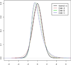
Figure 1: Densities of residuals under the four alternative distributions.

Table B1: Average estimates (SE) and percent of samples with rejected model

	Private schools				Public schools
	$\bolds{\hat{\mu}_{1,S}=6.01\,(0.14),\hat{\mu}_{1,C}=5.99\,(0.18)}$				$\bolds{\hat{\mu}_{0,S}=7.34\,(0.13),\hat{\mu}_{0,C}=7.09\,(0.39)}$
ATE	$\bolds{\hat{\tau}_{S}=-1.32\,(0.20);\hat{\tau}_{C}=-1.10\,(0.43)}$
Sig. level	0.10	0.05	0.025	0.01	0.10	0.05	0.025	0.01
Distribution A
K–S	100	100	099	096	75	64	55	52
C–M	100	100	100	100	91	87	79	72
A–D	100	100	100	100	94	90	88	83
	$\bolds{\hat{\mu}_{1,S}=5.96\,(0.19),\hat{\mu}_{1,C}=6.01\,(0.15)}$				$\bolds{\hat{\mu}_{0,S}=6.84\,(0.10),\hat{\mu}_{0,C}=6.89\,(0.26)}$
ATE	$\bolds{\hat{\tau}_{S}=-0.88\,(0.22);\hat{\tau}_{C}=-0.88\,(0.31)}$
Sig. level	0.10	0.05	0.025	0.01	0.10	0.05	0.025	0.01
Distribution B
K–S	100	100	100	099	72	64	51	47
C–M	100	100	100	100	83	77	66	63
A–D	100	100	100	100	92	79	76	70
	$\bolds{\hat{\mu}_{1,S}=5.42\,(0.20),\hat{\mu}_{1,C}=5.49\,(0.67)}$				$\bolds{\hat{\mu}_{0,S}=6.76\,(0.08),\hat{\mu}_{0,C}=6.90\,(0.46)}$
ATE	$\bolds{\hat{\tau}_{S}=-1.34\,(0.22);\hat{\tau}_{C}=-1.41\,(0.83)}$
Sig. level	0.10	0.05	0.025	0.01	0.10	0.05	0.025	0.01
Distribution C
K–S	100	100	100	100	67	56	40	39
C–M	100	100	100	100	85	75	71	67
A–D	100	100	100	100	93	88	79	78

Table B1 shows the percentage of samples that the misspecified models have been rejected by the three test statistics when using the conventional 10%, 5%, 2.5% and 1% significance levels. The percentages estimate the power of the tests. As can be seen, all the tests reject the three misspecified models for the private schools in literally all the samples, and the powers of the Cramer–von Misses test, and, in particular, the powers of the Anderson–Darling test are acceptable for the three misspecified models for the public schools as well. We mention in this regard that the three misspecified distributions were chosen to be sufficiently close to the normal distribution (see Figure 1). Further empirical results not shown indicate that for only mild larger distortions from the normal distribution, the powers of the three tests for the public schools are likewise close to 1.

Table B1 also shows the average of the estimates of the mean score in each group and the ATE, and the corresponding standard errors of the estimates (in parenthesis), over the 100 data sets. The empirical averages deviate now significantly from the corresponding true values ($\mu^{1}=6.10$, $\mu^{0}=7.05$; $\Delta=-0.95$) under all the three misspecified models and with larger standard errors than under the correct model. However, the estimates of the ATE are still highly negative, as under the correct model.

The conclusion from this simulation study is that even mild distortions from normality can affect the magnitude of the estimates of the ATE (but not their sign), but these mild distortions can be detected by the goodness-of-fit test statistics.

References

- Abadie and Imbens (2006) {barticle}[mr] \bauthor\bsnmAbadie, \bfnmAlberto\binitsA. and \bauthor\bsnmImbens, \bfnmGuido W.\binitsG. W. (\byear2006). \btitleLarge sample properties of matching estimators for average treatment effects. \bjournalEconometrica \bvolume74 \bpages235–267. \biddoi=10.1111/j.1468-0262.2006.00655.x, mr=2194325 \endbibitem
- Adams and Wu (2002) {bmisc}[auto:STB—2010-11-18—09:18:59] \bauthor\bsnmAdams, \bfnmRay\binitsR. and \bauthor\bsnmWu, \bfnmM.\binitsM., eds. (\byear2002). \bhowpublishedPISA 2000 Technical report, OECD, Paris. \endbibitem
- Azzalini and Capitanio (2003) {barticle}[mr] \bauthor\bsnmAzzalini, \bfnmAdelchi\binitsA. and \bauthor\bsnmCapitanio, \bfnmAntonella\binitsA. (\byear2003). \btitleDistributions generated by perturbation of symmetry with emphasis on a multivariate skew -distribution. \bjournalJ. R. Stat. Soc. Ser. B Stat. Methodol. \bvolume65 \bpages367–389. \biddoi=10.1111/1467-9868.00391, mr=1983753 \endbibitem
- Babu and Feigelson (2006) {bincollection}[auto:STB—2010-11-18—09:18:59] \bauthor\bsnmBabu, \bfnmG. J.\binitsG. J. and \bauthor\bsnmFeigelson, \bfnmE. D.\binitsE. D. (\byear2006). \btitleAstrostatistics: Goodness-of-fit and all that! In \bbooktitleAstronomical Data Analysis Software and Systems XV, ASP Conference Series (\beditorC. Gabriel, C. Arviset, D. Ponz and E. Solano, eds.) \bvolume351 \bpages127–136. \bpublisherAstronomical Society of the Pacific, \baddressSan Francisco. \endbibitem
- Babu and Rao (2004) {barticle}[mr] \bauthor\bsnmBabu, \bfnmG. Jogesh\binitsG. J. and \bauthor\bsnmRao, \bfnmC. R.\binitsC. R. (\byear2004). \btitleGoodness-of-fit tests when parameters are estimated. \bjournalSankhyā \bvolume66 \bpages63–74. \bidmr=2082908 \endbibitem
- Brewer (1963) {barticle}[mr] \bauthor\bsnmBrewer, \bfnmK. R. W.\binitsK. R. W. (\byear1963). \btitleRatio estimation and finite populations: Some results deducible from the assumption of an underlying stochastic process. \bjournalAustral. J. Statist. \bvolume5 \bpages93–105. \bidmr=0182078 \endbibitem
- Dronkers and Avram (2010) {barticle}[auto:STB—2010-11-18—09:18:59] \bauthor\bsnmDronkers, \bfnmJ.\binitsJ. and \bauthor\bsnmAvram, \bfnmS.\binitsS. (\byear2010). \btitleA cross-national analysis of the relations of school choice and effectiveness differences between private-dependent and public schools. \bjournalEducational Research and Evaluation \bvolume16 \bpages151–175. \endbibitem
- Gelman et al. (2004) {bbook}[mr] \bauthor\bsnmGelman, \bfnmAndrew\binitsA., \bauthor\bsnmCarlin, \bfnmJohn B.\binitsJ. B., \bauthor\bsnmStern, \bfnmHal S.\binitsH. S. and \bauthor\bsnmRubin, \bfnmDonald B.\binitsD. B. (\byear2004). \btitleBayesian Data Analysis, \bedition2nd ed. \bpublisherChapman & Hall/CRC, \baddressBoca Raton, FL. \bidmr=2027492 \endbibitem
- Greenlees, Reece and Zieschang (1982) {barticle}[auto:STB—2010-11-18—09:18:59] \bauthor\bsnmGreenlees, \bfnmJ. S.\binitsJ. S., \bauthor\bsnmReece, \bfnmW. S.\binitsW. S. and \bauthor\bsnmZieschang, \bfnmK. D.\binitsK. D. (\byear1982). \btitleImputation of missing values when the probability of response depends on the variable being imputed. \bjournalJ. Amer. Statist. Assoc. \bvolume77 \bpages251–261. \endbibitem
- Hajek (1971) {bmisc}[mr] \bauthor\bsnmHajek, \bfnmJaroslav\binitsJ. (\byear1971). \bhowpublishedComment on “An essay on the logical foundations of survey sampling, part one”. In The Foundations of Survey Sampling (V. P. Godambe and D. A. Sprott, eds.) 236. Holt, Rinehart and Winston, Toronto, ON. \endbibitem
- Hanushek (2002) {bincollection}[auto:STB—2010-11-18—09:18:59] \bauthor\bsnmHanushek, \bfnmE.\binitsE. (\byear2002). \btitlePublicly provided education. In \bbooktitleHandbook of Public Economics (\beditorA. J. Auerbach and M. Feldstein, eds.) \bpages2045–2141. \bpublisherNorth-Holland, \baddressAmsterdam. \endbibitem
- Heckman and Vytlacil (2006) {bincollection}[auto:STB—2010-11-18—09:18:59] \bauthor\bsnmHeckman, \bfnmJ.\binitsJ. and \bauthor\bsnmVytlacil, \bfnmE.\binitsE. (\byear2006). \btitleEconometric evaluation of social programs. In \bbooktitleHandbook of Econometrics \bvolume6B (\beditorJ. Heckman and E. Leamer, eds.) \bpages4810–4861. \bpublisherNorth-Holland, \baddressAmsterdam. \endbibitem
- Hoxby (2000) {barticle}[auto:STB—2010-11-18—09:18:59] \bauthor\bsnmHoxby, \bfnmC. M.\binitsC. M. (\byear2000). \btitleDoes competition among public schools benefit students and taxpayers? \bjournalThe American Economic Review \bvolume90 \bpages1209–1238. \endbibitem
- Imbens and Angrist (1994) {barticle}[auto:STB—2010-11-18—09:18:59] \bauthor\bsnmImbens, \bfnmG.\binitsG. and \bauthor\bsnmAngrist, \bfnmJ.\binitsJ. (\byear1994). \btitleIdentification and estimation of local average treatment effects. \bjournalEconometrics \bvolume62 \bpages467–475. \endbibitem
- Landsman (2008) {bmisc}[auto:STB—2010-11-18—09:18:59] \bauthor\bsnmLandsman, \bfnmV.\binitsV. (\byear2008). \bhowpublishedEstimation of treatment effects in observational studies by recovering the assignment probabilities and the population model. Ph.D. dissertation, Hebrew Univ. Jerusalem, Israel. \endbibitem
- Lee and Berger (2001) {barticle}[mr] \bauthor\bsnmLee, \bfnmJaeyong\binitsJ. and \bauthor\bsnmBerger, \bfnmJames O.\binitsJ. O. (\byear2001). \btitleSemiparametric Bayesian analysis of selection models. \bjournalJ. Amer. Statist. Assoc. \bvolume96 \bpages1397–1409. \biddoi=10.1198/016214501753382318, mr=1946585 \endbibitem
- Little (2004) {barticle}[mr] \bauthor\bsnmLittle, \bfnmRoderick J.\binitsR. J. (\byear2004). \btitleTo model or not to model? Competing modes of inference for finite population sampling. \bjournalJ. Amer. Statist. Assoc. \bvolume99 \bpages546–556. \biddoi=10.1198/016214504000000467, mr=2109316 \endbibitem
- Lunceford and Davidian (2004) {barticle}[auto:STB—2010-11-18—09:18:59] \bauthor\bsnmLunceford, \bfnmJ. K.\binitsJ. K. and \bauthor\bsnmDavidian, \bfnmM.\binitsM. (\byear2004). \btitleStratification and weighting via the propensity score in estimation of causal treatment effects: A comparative study. \bjournalStat. Med. \bvolume23 \bpages2937–2960. \endbibitem
- Maddala (1983) {bbook}[mr] \bauthor\bsnmMaddala, \bfnmG. S.\binitsG. S. (\byear1983). \btitleLimited-Dependent and Qualitative Variables in Econometrics. \bseriesEconometric Society Monographs in Quantitative Economics \bvolume3. \bpublisherCambridge Univ. Press, \baddressCambridge. \bidmr=0799154 \endbibitem
- McCaffrey, Ridgeway and Morral (2004) {barticle}[auto:STB—2010-11-18—09:18:59] \bauthor\bsnmMcCaffrey, \bfnmD.\binitsD., \bauthor\bsnmRidgeway, \bfnmG.\binitsG. and \bauthor\bsnmMorral, \bfnmA.\binitsA. (\byear2004). \btitlePropensity score estimation with boosted regression for evaluating causal effects in observational studies. \bjournalPsychological Methods \bvolume9 \bpages403–425. \endbibitem
- Pfeffermann and Landsman (2011) {bmisc}[auto:STB—2010-11-18—09:18:59] \bauthor\bsnmPfeffermann, \bfnmD.\binitsD. and \bauthor\bsnmLandsman, \bfnmV.\binitsV. (\byear2011). \bhowpublishedSupplement to “Are private schools better than public schools? Appraisal for Ireland by methods for observational studies.” DOI:10.1214/11-AOAS456SUPP. \endbibitem
- Pfeffermann and Sverchkov (2003) {bincollection}[mr] \bauthor\bsnmPfeffermann, \bfnmDanny\binitsD. and \bauthor\bsnmSverchkov, \bfnmM. Yu.\binitsM. Y. (\byear2003). \btitleFitting generalized linear models under informative sampling. In \bbooktitleAnalysis of Survey Data (Southampton, 1999) \bpages175–195. \bpublisherWiley, \baddressChichester. \biddoi=10.1002/0470867205.ch12, mr=1978851 \endbibitem
- Pfeffermann and Sverchkov (2009) {bincollection}[auto:STB—2010-11-18—09:18:59] \bauthor\bsnmPfeffermann, \bfnmD.\binitsD. and \bauthor\bsnmSverchkov, \bfnmM.\binitsM. (\byear2009). \btitleInference under informative sampling. In \bbooktitleSample Surveys: Inference and Analysis. \bseriesHandbook of Statistics \bvolume29B (\beditorD. Pfeffermann and C. R. Rao, eds.) \bpages455–487. \bpublisherNorth-Holland, \baddressAmsterdam. \endbibitem
- Qin and Zhang (2007) {barticle}[mr] \bauthor\bsnmQin, \bfnmJing\binitsJ. and \bauthor\bsnmZhang, \bfnmBiao\binitsB. (\byear2007). \btitleEmpirical-likelihood-based inference in missing response problems and its application in observational studies. \bjournalJ. R. Stat. Soc. Ser. B Stat. Methodol. \bvolume69 \bpages101–122. \biddoi=10.1111/j.1467-9868.2007.00579.x, mr=2301502 \endbibitem
- R Development Core Team (2004) {bmisc}[auto:STB—2010-11-18—09:18:59] \borganizationR Development Core Team (\byear2004). \bhowpublishedR: A Language and Environment for Statistical Computing. R Foundation for Statistical Computing, Vienna, Austria. \endbibitem
- Rosenbaum (2002) {bbook}[mr] \bauthor\bsnmRosenbaum, \bfnmPaul R.\binitsP. R. (\byear2002). \btitleObservational Studies, \bedition2nd ed. \bpublisherSpringer, \baddressNew York. \bidmr=1899138 \endbibitem
- Rosenbaum and Rubin (1983) {barticle}[mr] \bauthor\bsnmRosenbaum, \bfnmPaul R.\binitsP. R. and \bauthor\bsnmRubin, \bfnmDonald B.\binitsD. B. (\byear1983). \btitleThe central role of the propensity score in observational studies for causal effects. \bjournalBiometrika \bvolume70 \bpages41–55. \biddoi=10.1093/biomet/70.1.41, mr=0742974 \endbibitem
- Rotnitzky and Robins (1997) {barticle}[auto:STB—2010-11-18—09:18:59] \bauthor\bsnmRotnitzky, \bfnmA.\binitsA. and \bauthor\bsnmRobins, \bfnmJ.\binitsJ. (\byear1997). \btitleAnalysis of semi-parametric regression models with non-ignorable non-response. \bjournalStat. Med. \bvolume16 \bpages81–102. \endbibitem
- Rubin (1974) {barticle}[auto:STB—2010-11-18—09:18:59] \bauthor\bsnmRubin, \bfnmD. B.\binitsD. B. (\byear1974). \btitleEstimating causal effects of treatments in randomized and nonrandomized studies. \bjournalJ. Educational Psychology \bvolume66 \bpages688–701. \endbibitem
- Särndal, Swensson and Wretman (1992) {bbook}[mr] \bauthor\bsnmSärndal, \bfnmCarl-Erik\binitsC.-E., \bauthor\bsnmSwensson, \bfnmBengt\binitsB. and \bauthor\bsnmWretman, \bfnmJan\binitsJ. (\byear1992). \btitleModel Assisted Survey Sampling. \bpublisherSpringer, \baddressNew York. \bidmr=1140409 \endbibitem
- Smith and Sugden (1988) {barticle}[auto:STB—2010-11-18—09:18:59] \bauthor\bsnmSmith, \bfnmT. M. F.\binitsT. M. F. and \bauthor\bsnmSugden, \bfnmR. A.\binitsR. A. (\byear1988). \btitleSampling and assignment mechanisms in experiments, surveys and observational studies. \bjournalInternat. Statist. Rev. \bvolume56 \bpages165–180. \endbibitem
- StataCorp (2004) {bmisc}[auto:STB—2010-11-18—09:18:59] \borganizationStataCorp (\byear2004). \bhowpublishedStata Statistical Software: Release 7. StataCorp LP, College Station, TX. \endbibitem
- Stephens (1986) {bincollection}[auto:STB—2010-11-18—09:18:59] \bauthor\bsnmStephens, \bfnmM. A.\binitsM. A. (\byear1986). \btitleTests based on EDF statistics. In \bbooktitleGoodness-of-Fit Techniques (\beditorR. B. D’Agostino and M. A. Stephens, eds.) \bpages97–193. \bpublisherDekker, \baddressNew York. \endbibitem