Pairing correlations and odd-even staggering in reaction cross sections
of weakly bound nuclei

Abstract

We investigate the odd-even staggering (OES) in reaction cross sections of weakly bound nuclei with a Glauber theory, taking into account the pairing correlation with the Hartree-Fock-Bogoliubov (HFB) method. We first discuss the pairing gap in extremely weakly bound nuclei and show that the pairing gap persists in the limit of zero separation energy limit even for single-particle orbits with the orbital angular momenta $l=0$ and $l=1$. We then introduce the OES parameter defined as the second derivative of reaction cross sections with respect to the mass number, and clarify the relation between the magnitude of OES and the neutron separation energy. We find that the OES parameter increases considerably in the zero separation energy limit for $l=0$ and $l=1$ single-particle states, while no increase is found for higher angular momentum orbits with e.g., $l=3$. We point out that the increase of OES parameter is also seen in the experimental reaction cross sections for Ne isotopes, which is well accounted for by our calculations.

I Introduction

Reaction cross sections $\sigma_{R}$ of unstable nuclei provide a powerful tool to study the structure of unstable nuclei such as density distribution and deformation Tani85 ; Mitt87 ; Ozawa00 . For instance, a largely extended structure, referred to as “halo”, of unstable nuclei such as ¹¹Li Tani85 , ¹¹Be Fuk91 , and ^17,19C Ozawa00 has been found with such measurements. The halo structure is one of the characteristic features of weakly bound nuclei, and has attracted lots of attention (see Ref. Naka09 for a recent discovery of halo structure in ³¹Ne nucleus).

Experimentally large odd-even staggering (OES) phenomena have been revealed in reaction cross sections of unstable nuclei close to the neutron drip line, e.g., in the isotopes ^14,15,16C FYZ04 , ^18,19,20C Ozawa00 , ^28,29,30NeTakechi10 , ^30,31,32Ne Takechi10 , and ^36,37,38Mg Takechi11 . In Ref. HS11 , we have argued that the pairing correlations play an essential role in these OES. That is, the OES in reaction cross sections is intimately related to the so called pairing anti-halo effect discussed in Ref. Benn00 . On the other hand, there have been contradictory arguments whether the pairing gap disappears Hamamoto or persistsZMM11 ; Yamagami05 when a nucleus reaches at the neutron drip line, i.e., the single-particle energy of the last occupied orbit approaches the zero energy. If the pairing gap disappeared, the OES effect might be either quenched or disappeared completely, unless the deformation parameter is significantly different among the neighboring nuclei Minomo11 .

In this paper, we first discuss the pairing correlations close to the zero energy by the Hartree-Fock Bogoliubov (HFB) method. We carry out HFB calculations for the neutron 3s_1/2 orbit in ⁷⁶Cr changing the separation energy in a mean field potential, and examine different definitions for an effective pairing gap parameter. This problem is also related with the superfluidity of neutron gases in the outer crust of neutron stars Schuck11 . The second motivation of this work, in addition to giving the details of the analysis in Ref. HS11 , is to propose a formula to measure the odd-even staggering in the reaction cross sections. Notice that the OES of the isotope shift of stable nuclei has been discussed mostly to clarify the deformation changes in odd-mass and even-mass nuclei BM75 . The present issue of OES in the reaction cross sections has a similar aspect to the previous study in Ref. BM75 in one sense, but different in another aspect since it aims at studying the existence of the pairing correlation in nuclei close to the neutron drip line.

The paper is organized as follows. In Sec. II, we discuss the pairing correlation in neutron-rich nuclei using the HFB method. In Sec. III, we apply a Glauber theory in order to calculate reaction cross sections. We introduce the OES parameter for reaction cross sections, and discuss it in relation with the pairing correlations in weakly bound nuclei. We then summarize the paper in Sec. IV.

II Pairing gap at neutron drip line

In the coordinate space representation, the HFB equations read DFT84 ; DNW96 ; B00

$$\left(\begin{array}[]{cc}\hat{h}-\lambda&\Delta(\mbox{\boldmath$r$})\\ \Delta(\mbox{\boldmath$r$})&-\hat{h}+\lambda\end{array}\right)\left(\begin{array}[]{c}u_{i}(\mbox{\boldmath$r$})\\ v_{i}(\mbox{\boldmath$r$})\end{array}\right)=E_{i}\left(\begin{array}[]{c}u_{i}(\mbox{\boldmath$r$})\\ v_{i}(\mbox{\boldmath$r$})\end{array}\right),$$ (7)

where

$$\hat{h}=-\frac{\hbar^{2}}{2m}\nabla^{2}+V(\mbox{\boldmath$r$}),$$ (8)

is the mean-field Hamiltonian, $m$ being the nucleon mass. $V(\mbox{\boldmath$r$})$ and $\Delta(\mbox{\boldmath$r$})$ are the mean-field and the pairing potentials, respectively, and $E_{i}$ is a quasi-particle energy. Here, we have assumed that the nucleon-nucleon interaction is a zero range force so that these potentials are local. The upper component of the pair wave function $u_{i}(\mbox{\boldmath$r$})$ is a non-localized wave function if the quasi-particle energy $E_{i}$ is larger than the Fermi energy $|\lambda|$, while the lower component $v_{i}(\mbox{\boldmath$r$})$ is always localized. The pair potential $\Delta(\mbox{\boldmath$r$})$ in general has a larger surface diffuseness than the mean field potential $V(\mbox{\boldmath$r$})$, and goes beyond it due to the non-localized property of the upper component of the wave function $u_{i}(\mbox{\boldmath$r$})$, that is, due to the coupling to the continuum spectra DNW96 .

In the mean field approximation without the pairing correlations (i.e., $\Delta(\mbox{\boldmath$r$})=0$), the halo structure originates from an occupation of a weakly-bound $l=0$ or $l=1$ orbit by the valence nucleons near the threshold Riisager ; Sagawa93 . The asymptotic behavior of a single particle wave function for $s$ wave reads

$$\psi_{i}(r)\sim\exp(-\alpha_{i}r),$$ (9)

where $\alpha_{i}$ is defined as $\alpha_{i}=\sqrt{2m|\varepsilon_{i}|/\hbar^{2}}$ with the Hartree-Fock (HF) energy $\varepsilon_{i}$. The mean square radius of this wave function is then evaluated as

$$\langle r^{2}\rangle_{\rm HF}=\frac{\int r^{2}|\psi_{i}(r)|^{2}d\mbox{\boldmath$r$}}{\int|\psi_{i}(r)|^{2}d\mbox{\boldmath$r$}}\propto\frac{1}{\alpha_{i}^{2}}=\frac{\hbar^{2}}{2m|\varepsilon_{i}|},$$ (10)

which will diverge in the limit of vanishing separation energy, $|\varepsilon_{i}|\rightarrow 0$. It has been shown that this divergence occurs not only for $s$ wave but also for $p$ wave, although the dependence on $|\varepsilon_{i}|$ is now $\langle r^{2}\rangle_{\rm HF}\propto 1/\sqrt{|\varepsilon_{i}|}$ for $l=1$ Riisager .

In contrast, in the presence of the pairing correlations (i.e., $\Delta(\mbox{\boldmath$r$})\neq 0$), the lower component of the HFB wave function, which is relevant to the density distribution, behaves as DNW96

$$v_{i}(r)\propto\exp(-\beta_{i}r),$$ (11)

where $\beta_{i}$ is given by,

$$\beta_{i}=\sqrt{\frac{2m}{\hbar^{2}}(E_{i}-\lambda)},$$ (12)

using the quasi-particle energy $E_{i}$. With the canonical basis $\phi_{i}^{\rm(can)}(\mbox{\boldmath$r$})$ in the HFB theory, the quasi-particle energy may be approximately given by DNW96

$$E_{i}=\sqrt{(\varepsilon_{i}^{\rm(can)}-\lambda)^{2}+(\Delta_{i}^{\rm(can)})^{2}},$$ (13)

where $\varepsilon_{i}^{\rm(can)}\equiv\langle\phi_{i}^{(\rm can)}|\hat{h}|\phi_{i}^{(\rm can)}\rangle$ and $\Delta_{i}^{\rm(can)}\equiv\langle\phi_{i}^{(\rm can)}|\Delta(\mbox{\boldmath$r$})|\phi_{i}^{(\rm can)}\rangle$. In the zero binding limit, $\varepsilon_{i}^{(\rm can)}\sim 0$ and $\lambda\sim 0$, the asymptotic behavior of the wave function $v_{i}(r)$ is therefore determined by the gap parameter as,

$$v_{i}(r)\propto\exp\left[\left(-\sqrt{\frac{2m}{\hbar^{2}}\Delta_{i}^{(\rm can)}}\right)r\right].$$ (14)

The radius of the HFB wave function will then be given in the limit of small separation energy $|\varepsilon_{i}^{(\rm can)}|\rightarrow 0$ as

$$\langle r^{2}\rangle_{\rm HFB}=\frac{\int r^{2}|v_{i}(r)|^{2}d{\mbox{\boldmath$r$}}}{\int|v_{i}(r)|^{2}d\mbox{\boldmath$r$}}\propto\frac{1}{\beta_{i}^{2}}\rightarrow\frac{\hbar^{2}}{2m\Delta_{i}^{(\rm can)}}.$$ (15)

If the gap parameter $\Delta_{i}^{(\rm can)}$ stays finite in the zero energy limit of $\varepsilon_{i}^{(\rm can)}$, the extremely large extension of a halo wave function in the HF field will be reduced substantially by the pairing correlations and the root-mean-square (rms) radius will not diverge. This is referred to as the anti-halo effect due to the pairing correlations Benn00 . It was shown in Ref.  HS11 that this is the main reason for the observed OES in the reactions cross sections of several drip line nuclei.

In order to study the behavior of the pairing gap in weakly bound nuclei, we carry out HFB calculations for the neutrons in ⁷⁶Cr nucleus. To this end, we use a spherical Woods-Saxon (WS) potential,

$$V(r)=V_{0}f(r)-\frac{V_{\rm ls}}{r}\frac{df(r)}{dr}\,\mbox{\boldmath$l$}\cdot\mbox{\boldmath$s$},$$ (16)

with

$$f(r)=\frac{1}{1+\exp[(r-R_{0})/a]},$$ (17)

for the mean-field potential $V(r)$. Following Ref. YS08 , we take $V_{0}=-51+30(N-Z)/A$ MeV, $R_{0}=1.27A^{1/3}$ fm, $V_{\rm ls}=-0.71V_{0}$ MeV$\cdot$fm², and $a$=0.67 fm. For the HFB calculations, we use a density-dependent contact pairing interaction of surface type, with which the pairing potential is given by

$$\Delta(r)=\frac{V_{\rm pair}}{2}\left(1-\frac{\rho(r)}{\rho_{0}}\right)\,\tilde{\rho}_{n}(r).$$ (18)

Here, $\rho(r)$ and $\tilde{\rho}_{n}(r)$ are the total particle density and the neutron pairing density, respectively, given by

$$\rho(r) = \sum_{i=n,p}|v_{i}(\mbox{\boldmath$r$})|^{2},$$ (19)

$$\tilde{\rho}_{n}(r) = -\sum_{i=n}u_{i}^{*}(\mbox{\boldmath$r$})v_{i}(\mbox{\boldmath$r$}).$$ (20)

We again follow Ref. YS08 and take $\rho_{0}$=0.16 fm^-3 and $V_{\rm pair}=-420$ MeV$\cdot$fm³ with the energy cut off of 50 MeV above the Fermi energy. In order to construct the proton density, we use the same mean-field potential as in Eq. (16), but with $V_{0}=-51-30(N-Z)/A$ MeV. We also add the Coulomb potential for a uniform charge with a radius of $R_{0}$. We discretize the continuum spectra with the box boundary condition. We take the box size of $R_{\rm box}$=60 fm, and include the angular momentum up to $l=12$. Notice that we determine the pairing potential self-consistently in this model according to Eq. (18), although the Woods-Saxon potential is fixed for the mean-field part. The Fermi energy is also determined self-consistently according to the condition for the average particle number conservation,

$$\langle A\rangle=\int\rho(r)d\mbox{\boldmath$r$}=\int\sum_{i}|v_{i}(\mbox{\boldmath$r$})|^{2}d\mbox{\boldmath$r$}.$$ (21)

These self-consistencies are particularly important to increase the pairing gap for an extremely loosely bound orbit Yamagami05 .

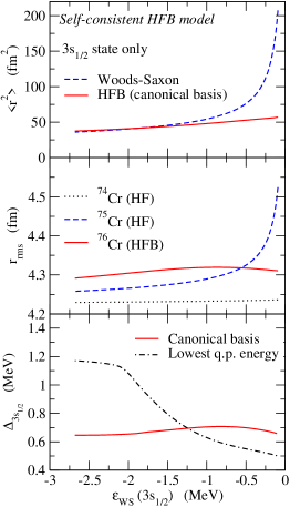
Figure 1: (Color online) The mean square radii and the paring gap for ⁷⁶Cr nucleus as a function of the single particle energy $\varepsilon_{\rm WS}$ for the 3s_1/2 orbit in a Woods-Saxon potential. The top panel shows the mean square radius of the 3s_1/2 wave function obtained with (the solid line) and without (the dashed line) the pairing correlation. The middle panel shows the root-means-square (rms) radii for ⁷⁴Cr (the dotted line), ⁷⁵Cr (the dashed line), and ⁷⁶Cr (the solid line). These are obtained with the Hartree-Fock (⁷⁴Cr and ⁷⁵Cr ) and the Hartree-Fock-Bogoliubov (⁷⁶Cr ) methods. The bottom panel shows the effective pairing gap for the 3s_1/2 state. The solid line is the pairing gap defined with the canonical basis, that is, the expectation value of the pair potential with respect to the canonical basis wave function for the 3s_1/2 state, while the dot-dashed line shows the lowest quasi-particle energy for the s_1/2 states.

The top panel of Fig. 1 shows the mean square radius of the 3$s_{1/2}$ state. In order to study the dependence on the binding energy, we vary the depth of the WS potential $V_{0}$ for neutron $s$ wave states while we keep the original value for the other angular momentum states. We also arbitrary change the single-particle energy for the 2d_5/2 state from $-0.38$ MeV to $-0.05$ MeV so that the 3s_1/2 state lies below the 2d_5/2 state. The dashed line is obtained with the single-particle wave function for the mean-field Hamiltonian $\hat{h}$, while the solid line is obtained with the wave function for the canonical basis in the HFB calculations. The radius of the single-particle wave function for the $s$-wave state increases rapidly as the single-particle energy $\epsilon$ approaches zero, and eventually diverges in the limit of $\epsilon_{\rm WS}\rightarrow 0$. In contrast, the HFB wave function shows only a moderate increase of the radius even in the limit of $\epsilon_{\rm WS}\rightarrow 0$. The middle panel of Fig. 1 shows the root-mean-square (rms) radius for the whole nucleus, by taking into account the contribution of the other orbits as well. For comparison, we also show the rms radii for ⁷⁴Cr and ⁷⁵Cr obtained with the same mean-field potential but without including the pairing correlation. Notice that the rms radius of ⁷⁶Cr is larger than that of ⁷⁵Cr in the range of $\epsilon_{\rm WS}<-0.56$ MeV. This is due to the coupling of single-particle wave functions to a larger model space, including continuum, induced by the pairing correlations. On the other hand, in the limit of $\epsilon_{\rm WS}\rightarrow 0$, the rms radius of ⁷⁵Cr shows a divergent feature while that of ⁷⁶Cr is almost constant. for the 3s_1/2 state. The solid line shows the pairing gap evaluated with the canonical basis, $\Delta_{i}^{(\rm can)}$ for $i=3$s_1/2, while the dot-dashed line is the lowest quasi-particle energy $E_{i}$. Notice that the right hand side of Eq. (13) is simply a diagonal component of the HFB Hamiltonian in the canonical basis, while the left hand side is obtained by diagonalizing the HFB matrixDNW96 . Due to the off-diagonal components, Eq. (13) holds only approximately, and thus $E_{i}$ may be smaller than $\Delta_{i}^{\rm{(can)}}$ in actual calculations. One can see in the figure that the effective pairing gaps persist even in the limit of $\epsilon_{\rm WS}\rightarrow 0$, leading to the reduction of the radius of HFB wave function as is shown in the top panel of Fig. 1.

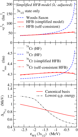
Figure 2: (Color online) Same as Fig. 1, but with the simplified HFB model, in which the pair potential is assumed to be proportional to the derivative of the Fermi function. Only the Fermi energy $\lambda$ is determined self-consistently in this model. The dot-dashed lines in the top and the middle panels denote the results of the self-consistent calculations shown in Fig. 1.

In the simplified HFB model of Ref. Hamamoto , it was claimed that the effective paring gap is diminished or quenched substantially for low $l$ orbits with $l=0$ and $l=1$. In this model, the radial dependence of the pairing field $\Delta(r)$ is fixed either as a Fermi-type function (volume-type) or a derivative of the Fermi function (surface-type) with the same surface diffuseness parameter as in the mean-field potential. Furthermore, the Fermi energy is set equal to the single-particle energy, $\epsilon$, for the mean-field Hamiltonian $\hat{h}$, that is, $\lambda=\epsilon$. The effective pairing gap is defined in Ref. Hamamoto to be identical to the corresponding quasi-particle energy. If the energy in the canonical basis were the same as the single-particle energy, Eq. (13) indeed yields

$$E_{i}=\Delta_{i}^{(\rm can)}.$$ (22)

Care must be needed, however, since in general $\epsilon_{i}^{(\rm can)}$ deviates from the single-particle energy, $\epsilon_{i}$ in the HFB. Moreover, when the effective gap is plotted as a function of $\epsilon$ as has been done in Ref. Hamamoto , setting $\lambda=\epsilon$ leads to a violation of particle number in this model, whose effect may be large in the limit of $\epsilon\to 0$.

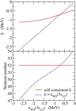
Figure 3: (Color online) The Fermi energy $\lambda$ and the neutron number calculated with the simplified HFB model. These are plotted as a function of the single particle energy $\epsilon_{\rm WS}$ for the 3s_1/2 orbit in a Woods-Saxon potential. The solid lines are obtained by adjusting the Fermi energy so that the neutron number is $N$=52, while the dashed lines are obtained by setting $\lambda=\epsilon_{\rm WS}$.

In order to investigate the consistency of the simplified model of Ref. Hamamoto , we repeat the same calculations shown in Fig. 1 by assuming that the pair potential $\Delta(r)$ is proportional to $r\cdot df/dr$, where $f(r)$ is given by Eq. (17). We use the proportional constant of $-1.107$ MeV, that leads to the same value for the average pairing gap,

$$\bar{\Delta}=\frac{\int^{\infty}_{0}r^{2}dr\,\Delta(r)\rho(r)}{\int^{\infty}_{0}r^{2}dr\,\rho(r)},$$ (23)

as that in the self-consistent calculations shown in Fig. 1 for $\epsilon_{\rm WS}(3s_{1/2})=-0.257$ MeV. We keep this value in varying the depth of the Woods-Saxon potential, $-V_{0}$.

We first keep the particle number to be a constant ($N$=52) and determine the Fermi energy self-consistently within this simplified model. Figure 2 show the results of such calculations. For comparison, the top and the middle panels also show by the dot-dashed lines the results of the self-consistent calculations, which have already been shown in Fig. 1. It is remarkable that this model yields a similar rms radius to that of the self-consistent calculation. The effective pairing gaps show somewhat different behavior from those in the self-consistent calculation, especially for the pairing gap defined with the canonical basis (see the bottom panel). However, it should be emphasized that the pairing gaps stay finite in this calculation in the limit of vanishing single-particle energy, as in the self-consistent calculation shown in Fig. 1. This implies that the self-consistency for the pair potential is not important, as far as the rms radius is concerned.

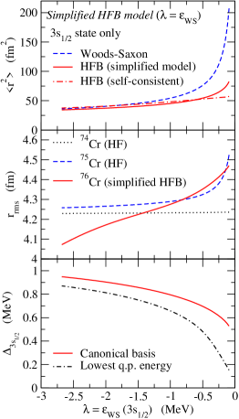
Figure 4: (Color online) Same as Fig. 2, but by fixing the Fermi energy to be the same as the single-particle energy for the 3s_1/2 state, $\lambda=\epsilon_{\rm WS}(3s_{1/2})$.

We next carry out the calculation by setting the Fermi energy to be the same as the single-particle energy for the 3s_1/2 state, $\lambda=\epsilon(3s_{1/2})$. In this calculation, the number of particle changes as we vary the depth of the Woods-Saxon potential. The Fermi energy $\lambda$ and the neutron number are shown in the upper and the lower panels of Fig. 3, respectively, by the dashed lines. For comparison, the figure also shows the results of the previous calculation shown in Fig. 2, that is, those obtained by adjusting the Fermi energy so that the neutron number is a constant (see the solid lines). The variation of the particle number is large, that is, from 47 to 54 in the range of single-particle energy shown in Fig. 3. The radii and the effective pairing gaps are shown in Fig. 4. As one can clearly see, this non-self-consistent calculation yields considerably different results from the self-consistent calculations. Firstly, the reduction of the mean square radius of the single-particle orbit is somewhat underestimated, although the effect is still large (see the top panel). Secondly, the rms radius obtained with this model is completely inconsistent with the result of the self-consistent calculation as shown in the middle panel. Lastly, the effective pairing gaps drops off in the limit of $\epsilon\to 0$ (see the bottom panel). Particularly, the lowest quasi-particle energy is substantially dismissed, that is a similar behavior as that shown in Ref. Hamamoto . Evidently, the claim of Ref. Hamamoto that the pairing gap disappears in the zero energy limit is an artifact of setting $\lambda=\epsilon$. If the Fermi energy is determined self-consistently for a given particle number, the effective pairing gap persists even if the pairing potential is pre-fixed as shown in Fig. 2.

III Odd-even staggering of reaction cross sections

Let us now investigate how the pairing correlation affects the reaction cross sections of weakly-bound nuclei. To this end, we use the Glauber theory Glauber ; BD04 ; OKYS01 ; OYS92 ; HSAK07 ; HSCB10 . In the optical limit approximation of the Glauber theory, the reaction cross section $\sigma_{R}$ can be calculated as OKYS01 ; OYS92 ; HSAK07 ; HSCB10 ,

$$\sigma_{R}=\int d\mbox{\boldmath$b$}\,\left(1-\left|e^{i\chi(\mbox{\boldmath$b$})}\right|^{2}\right),$$ (24)

with

$$i\chi(\mbox{\boldmath$b$})=-\int d\mbox{\boldmath$r$}d\mbox{\boldmath$r$}^{\prime}\rho_{P}(\mbox{\boldmath$r$})\rho_{T}(\mbox{\boldmath$r$}^{\prime})\Gamma_{NN}(\mbox{\boldmath$s$}-\mbox{\boldmath$s$}^{\prime}+\mbox{\boldmath$b$}).$$ (25)

Here, $\rho_{P}$ and $\rho_{T}$ are the projectile and the target densities, respectively, and $b$ is the impact parameter. $s$ and $\mbox{\boldmath$s$}^{\prime}$ are the transverse components of $r$ and $\mbox{\boldmath$r$}^{\prime}$, respectively, that is, $\mbox{\boldmath$s$}=(\mbox{\boldmath$r$}\cdot\mbox{\boldmath$e$}_{b})\,\mbox{\boldmath$e$}_{b}$ and $\mbox{\boldmath$s$}^{\prime}=(\mbox{\boldmath$r$}^{\prime}\cdot\mbox{\boldmath$e$}_{b})\,\mbox{\boldmath$e$}_{b}$, where $\mbox{\boldmath$e$}_{b}=\mbox{\boldmath$b$}/b$ is the unit vector parallel to $b$. $\Gamma_{NN}$ is the profile function for the $NN$ scattering, for which we assume to take a form of OKYS01 ; OYS92 ; HSAK07 ; HSCB10 ,

$$\Gamma_{NN}(\mbox{\boldmath$b$})=\frac{1-i\alpha}{4\pi\beta}\,\sigma_{NN}\exp\left(-\frac{b^{2}}{2\beta}\right),$$ (26)

with $\sigma_{NN}$ being the total $NN$ cross section.

It has been known that the optical limit approximation overestimates reaction cross sections for weakly-bound nuclei BES90 ; TUKS92 ; AKT96 ; AKTT96 ; AIS00 . In order to cure this problem, Abu-Ibrahim and Suzuki have proposed modifying the phase shift function $\chi(\mbox{\boldmath$b$})$ in Eq. (25) to AIS00

$$i\chi(\mbox{\boldmath$b$})=-\frac{1}{2}\int d\mbox{\boldmath$r$}\rho_{P}(\mbox{\boldmath$r$})$$

$$\times\left[1-\exp\left(-\int d\mbox{\boldmath$r$}^{\prime}\rho_{T}(\mbox{\boldmath$r$}^{\prime})\Gamma_{NN}(\mbox{\boldmath$s$}-\mbox{\boldmath$s$}^{\prime}+\mbox{\boldmath$b$})\right)\right]$$

$$-\frac{1}{2}\int d\mbox{\boldmath$r$}^{\prime}\rho_{T}(\mbox{\boldmath$r$}^{\prime})$$

$$\times\left[1-\exp\left(-\int d\mbox{\boldmath$r$}\rho_{P}(\mbox{\boldmath$r$})\Gamma_{NN}(\mbox{\boldmath$s$}^{\prime}-\mbox{\boldmath$s$}+\mbox{\boldmath$b$})\right)\right].$$ (27)

With this prescription, the effects of multiple scattering between a projectile nucleon and the target nucleus, and that between a target nucleon and the projectile nucleus, are included to some extent AIS00 .

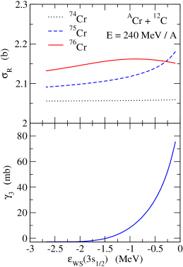
Figure 5: (Color online) (The upper panel) Reaction cross sections for ^74,75,76Cr + ¹²C reactions at $E$=240 MeV/nucleon, obtained with the modified optical limit approximation of the Glauber theory, Eq. (27). The density distributions for the ^74,75,76Cr are constructed from the HFB calculations shown in Fig. 1. (The lower panel) The staggering parameter defined by Eq. (28).

The upper panel of Fig. 5 shows the reaction cross sections for ^74,75,76Cr + ¹²C reactions at $E$=240 MeV/nucleon, obtained with the phase shift function given by Eq. (27). For the density of the Cr isotopes, we use the results of the HFB calculations shown in Fig. 1. For the density of the target nucleus ¹²C, we use the same density distribution as that given in Ref. OYS92 . In the actual calculation, we treat the proton-neutron and the proton-proton/neutron-neutron scattering separately and use the parameters given in Table I in Ref. AIHKS08 for the profile function $\Gamma_{NN}$. In order to evaluate the phase shift function, we use the two-dimensional Fourier transform technique BS95 . We give its explicit form in the Appendix. The reaction cross sections shown in Fig. 5 show a similar behavior as in the rms radii shown in the middle panel of Fig. 1, as is expected. That is, the reaction cross sections for ⁷⁶Cr and ⁷⁵Cr are inverted at a small biding energy, due to the pairing effect shown in Fig. 1. This leads to a large odd-even staggering in reaction cross sections for weakly bound nucleiHS11 .

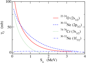
Figure 6: (Color online) The staggering parameter $\gamma_{3}$ defined by Eq. (28) as a function of the neutron separation energy S_n for the odd-mass nuclei. The solid and the dotted lines correspond to the reaction cross sections for ^22,23,24O+¹²C and ^74,75,76Cr+¹²C at $E$=240 MeV/nucleon, respectively. The dashed and the dot-dashed lines show the results for ^30,31,32Ne+¹²C at $E$=240 MeV/nucleon, in which the valence neutron in ³¹Ne occupies the 2p_3/2 or the 1f_7/2 orbits, respectively.

In order to quantify the OES of reaction cross sections, we introduce the staggering parameter defined by

$$\gamma_{3}=(-)^{A}\frac{\sigma_{R}(A+1)-2\sigma_{R}(A)+\sigma_{R}(A-1)}{2},$$ (28)

where $\sigma_{R}(A)$ is the reaction cross section of a nucleus with mass number $A$. We can define the same quantity also for rms radii. Notice that this staggering parameter is similar to the one often used for the OES of binding energy, that is, the pairing gap SDN98 ; DMNSS01 ; BBNSS09 . The lower panel of Fig. 5 shows the staggering parameter $\gamma_{3}$ for the ^74,75,76Cr nuclei as a function of the single-particle energy, $\epsilon_{\rm WS}$. One can clearly see that the staggering parameter $\gamma_{3}$ increases rapidly for small separation energies, and goes up to a large value reaching $\gamma_{3}\sim$ 80 mb.

In order to find out a general trend of the staggering parameter, Fig. 6 shows the value of $\gamma_{3}$ for various orbits with 2s_1/2, 3s_1/2, 2p_3/2 and 1f_7/2. The values for the 2s_1/2 and 2p_3/2 orbits correspond to the reaction cross sections for the ^22,23,24O and ^30,31,32Ne nuclei, respectively, calculated in Ref. HS11 . The value for the 1f_7/2 orbits corresponds to the reaction cross sections for ^30,31,32Ne nuclei, obtained with the diffuseness parameter of the mean-field Woods-Saxon potential of $a$=0.65 fm. One can clearly see that $\gamma_{3}$ for the low $l$ orbits with $l=0$ and $l=1$ show a rapid increase at small separation energies, the $l=0$ orbits increasing more rapidly than the $l=1$ orbit. In contrast, the high $l$ orbit with $l=3$ does not show any anomaly in the limit of $\epsilon\to 0$. These features are quite similar to the growth of a halo structure only in the low $l$ orbits due to a zero or small centrifugal barrier.

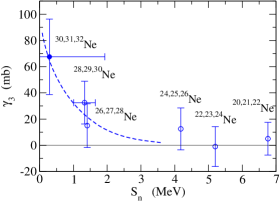
Figure 7: (Color online) The experimental staggering parameter $\gamma_{3}$ of reaction cross sections defined by Eq. (28) for the Ne isotopes with the ¹²C target at $E$=240 MeV/nucleon. This is plotted as a function of the neutron separation energy S_n of the odd-$A$ nuclei. The experimental data for the reaction cross sections are taken from Ref. Takechi10 , while the empirical separation energies are taken from Refs. Audi ; J07 . The dashed line is the calculated staggering parameter for the ^30,31,32Ne isotopes, assuming that the valence neutron in of ³¹Ne occupies the 2p${}_{3}/2$ orbit.

The experimental staggering parameters $\gamma_{3}$ are plotted in Fig. 7 for Ne isotopes as a function of the neutron separation energy for the odd-mass nuclei. We use the experimental reaction cross sections given in Ref. Takechi11 while we evaluate the separation energies with the empirical binding energies listed in Ref. Audi . For the neutron separation energy for the ³¹Ne nucleus, we use the value in Ref. J07 . The experimental uncertainties of the staggering parameter are obtained as

$$\delta\gamma_{3}=\frac{\sqrt{(\delta\sigma_{R}(A+1))^{2}+4(\delta\sigma_{R}(A))^{2}+(\delta\sigma_{R}(A-1))^{2}}}{2},$$ (29)

where $\delta\sigma_{R}(A)$ is the experimental uncertainty for the reaction cross section of a nucleus with mass number $A$. The figure also shows by the dashed line the calculated staggering parameter for the ^30,31,32Ne nuclei with the 2p_3/2 orbit, that has been shown also in Fig. 6. One sees that the experimental staggering parameter agrees with the calculated value for ^30,31,32Ne nuclei when one assumes that the valence neutron in ³¹Ne occupies the 2p_3/2 orbit. Furthermore, although the structure of lighter odd-A Ne isotopes is not known well, it is interesting to see that the empirical staggering parameters closely follow the calculated values for the 2p_3/2 orbit. This may indicate that the low-$l$ single-particle orbits are appreciably mixed in these Ne isotopes due to the deformation effectsH10 ; UHS11 .

IV Summary

We have studied the odd-even staggering (OES) of the reaction cross sections by using the Hartree-Fock-Bogoliubov model. To this end, we have introduced the staggering parameter $\gamma_{3}$ defined with a 3 point difference formula in order to clarify the relation between the magnitude of OES and the neutron separation energy. We have shown that the OES parameter increases largely for low-$l$ orbits with $l=0$ and $l=1$ at small separation energies. The experimental staggering parameter for the Ne isotopes show a similar increase. On the other hand, we have found that the staggering parameter stays almost a constant value, $\gamma_{3}\sim 2$ mb for higher $l$ orbits with e.g., $l=3$. The increase of $\gamma_{3}$ is induced by the finite pairing correlations in the zero separation energy limit. In this respect, we have shown that the effective pairing gap for the 3s_1/2 orbit in the ⁷⁶Cr nucleus persists even in the limit of vanishing separation energy. This remains the same even if the pair potential is prefixed, as long as the chemical potential is adjusted to keep the particle number to be the same. We have shown that such simplified HFB model well reproduces the results of the self-consistent HFB model for the root-mean-square radius.

The staggering parameter proposed in this paper provides a good measure for the OES of reaction cross sections. Further systematic experimental studies would be helpful in order to clarify the pairing correlations in weakly-bound nuclei and in the limit of zero neutron separation energy.

Appendix A Evaluation of phase shift function with the Fourier transform method

In this paper, we evaluate the phase shift functions given by Eqs. (25) and (27) using the Fourier transform technique BS95 . First we notice that Eq. (25) can be expressed as

$$i\chi(\mbox{\boldmath$b$})=-\int d\mbox{\boldmath$s$}d\mbox{\boldmath$s$}^{\prime}\rho^{(z)}_{P}(\mbox{\boldmath$s$})\rho^{(z)}_{T}(\mbox{\boldmath$s$}^{\prime})\Gamma_{NN}(\mbox{\boldmath$s$}-\mbox{\boldmath$s$}^{\prime}+\mbox{\boldmath$b$}),$$ (30)

with

$$\rho^{(z)}_{P}(\mbox{\boldmath$s$})\equiv\int dz\,\rho_{P}(\mbox{\boldmath$s$},z),~{}~{}~{}\rho^{(z)}_{T}(\mbox{\boldmath$s$}^{\prime})\equiv\int dz\,\rho_{T}(\mbox{\boldmath$s$}^{\prime},z).$$ (31)

The two-dimensional Fourier transform of $i\chi(\mbox{\boldmath$b$})$ in Eq. (25) then reads

$$i\tilde{\chi}(\mbox{\boldmath$q$}) = \int d\mbox{\boldmath$b$}\,i\chi(\mbox{\boldmath$b$})\,e^{i\mbox{\boldmath$q$}\cdot\mbox{\boldmath$b$}},$$

$$= -\int d\mbox{\boldmath$b$}\,e^{i\mbox{\boldmath$q$}\cdot(\mbox{\boldmath$b$}+\mbox{\boldmath$s$}-\mbox{\boldmath$s$}^{\prime})}\,\Gamma_{NN}(\mbox{\boldmath$b$}+\mbox{\boldmath$s$}-\mbox{\boldmath$s$}^{\prime})$$

$$\times \int d\mbox{\boldmath$s$}\,e^{-i\mbox{\boldmath$q$}\cdot\mbox{\boldmath$s$}}\,\rho^{(z)}_{P}(\mbox{\boldmath$s$})\int d\mbox{\boldmath$s$}^{\prime}\,e^{i\mbox{\boldmath$q$}\cdot\mbox{\boldmath$s$}^{\prime}}\,\rho^{(z)}_{T}(\mbox{\boldmath$s$}^{\prime}),$$ (33)

$$= -\tilde{\Gamma}_{NN}(\mbox{\boldmath$q$})(\tilde{\rho}_{P}^{(z)}(\mbox{\boldmath$q$}))^{*}\tilde{\rho}_{T}^{(z)}(\mbox{\boldmath$q$}),$$ (34)

where $\tilde{\Gamma}_{NN},\tilde{\rho}_{P}^{(z)}$, and $\tilde{\rho}_{T}^{(z)}$ are the two-dimensional Fourier transform of ${\Gamma}_{NN},{\rho}_{P}^{(z)}$, and ${\rho}_{T}^{(z)}$, respectively. For the profile function given by Eq. (26), its Fourier transform reads,

$$\tilde{\Gamma}_{NN}(q)=\frac{1-i\alpha}{4\pi\beta}\,\sigma_{NN}\cdot 2\beta^{2}\pi\exp\left(-\frac{\beta^{2}q^{2}}{2}\right).$$ (35)

The Fourier transform of the density distribution is evaluated as

$$\tilde{\rho}^{(z)}(\mbox{\boldmath$q$})=\int dzd\mbox{\boldmath$s$}\,e^{i\mbox{\boldmath$q$}\cdot\mbox{\boldmath$s$}}\,\rho(\mbox{\boldmath$s$},z)=\tilde{\rho}(\mbox{\boldmath$Q$}),$$ (36)

where $\tilde{\rho}(\mbox{\boldmath$Q$})$ is the three-dimensional Fourier transform of the density at $\mbox{\boldmath$Q$}=(\mbox{\boldmath$q$},Q_{z}=0)$. For a spherical density, $\rho(r)$, $\tilde{\rho}(\mbox{\boldmath$Q$})$ depends only on $|\mbox{\boldmath$Q$}|=q$, that is,

$$\tilde{\rho}^{(z)}(\mbox{\boldmath$q$})=\tilde{\rho}(q)=4\pi\int^{\infty}_{0}r^{2}dr\,\rho(r)j_{0}(qr),$$ (37)

where $j_{0}(qr)$ is the spherical Bessel function of zero-th order. Taking the inverse Fourier transform of Eq. (34), the phase shift function is calculated as

$$i\chi(\mbox{\boldmath$b$}) = -\int\frac{d\mbox{\boldmath$q$}}{(2\pi)^{2}}\,\tilde{\Gamma}_{NN}(q)\tilde{\rho}_{P}(q)\tilde{\rho}_{T}(q)e^{-i\mbox{\boldmath$q$}\cdot\mbox{\boldmath$b$}},$$ (38)

$$= -\int^{\infty}_{0}\frac{qdq}{2\pi}\,\tilde{\Gamma}_{NN}(q)\tilde{\rho}_{P}(q)\tilde{\rho}_{T}(q)J_{0}(qb),$$ (39)

where $J_{0}(qb)$ is the Bessel function of zero-th order. A similar technique has been used to evaluate a double folding potential in heavy-ion reactions SL79 ; BS97 ; KOBO07 .

One can apply the same method to evaluate the phase shift function given by Eq. (27). First notice that

$$\Gamma_{NT}(\mbox{\boldmath$b$}) \equiv 1-\exp\left(-\int d\mbox{\boldmath$r$}^{\prime}\rho_{T}(\mbox{\boldmath$r$}^{\prime})\Gamma_{NN}(\mbox{\boldmath$b$}-\mbox{\boldmath$s$}^{\prime})\right),$$

$$= 1-\exp\left(-\int^{\infty}_{0}\frac{qdq}{2\pi}\,\tilde{\Gamma}_{NN}(q)\tilde{\rho}_{T}(q)J_{0}(qb)\right),$$

depends only on $b=|\mbox{\boldmath$b$}|$. This leads to

$$i\chi(b) = -\frac{1}{4\pi}\int^{\infty}_{0}qdq\,\tilde{\Gamma}_{NT}(q)\tilde{\rho}_{P}(q)J_{0}(qb)$$ (42)

$$-\frac{1}{4\pi}\int^{\infty}_{0}qdq\,\tilde{\Gamma}_{NP}(q)\tilde{\rho}_{T}(q)J_{0}(qb),$$

where $\tilde{\Gamma}_{NT}(q)$ is calculated as

$$\tilde{\Gamma}_{NT}(q)=2\pi\int^{\infty}_{0}bdb\,\Gamma_{NT}(b)J_{0}(qb).$$ (43)

References

- (1) I. Tanihata et al., Phys. Rev. Lett. 55, 2676 (1985); Phys. Lett. B206, 592 (1988).
- (2) W. Mittig et al., Phys. Rev. Lett. 59, 1889 (1987).
- (3) A. Ozawa et al., Nucl. Phys. A691, 599 (2001).
- (4) M. Fukuda et al., Phys. Lett. B268, 339 (1991).
- (5) T. Nakamura et al., Phys. Rev. Lett. 103, 262501 (2009).
- (6) D.Q. Fang et al., Phys. Rev. C69, 034613 (2004).
- (7) M. Takechi et al., Nucl. Phys. A834, 412c(2010), and private communication.
- (8) M. Takechi et al., private communication.
- (9) K. Hagino and H. Sagawa, Phys. Rev. C84, 011303(R) (2011).
- (10) K. Bennaceur, J. Dobaczewski and M. Ploszajczak, Phys. Lett. B496, 154 (2000).
- (11) I. Hamamoto and B. R. Mottelson, Phys. Rev. C69, 064302 (2004).; I. Hamamoto and H. Sagawa, Phys. Rev. C70, 034317 (2004).
- (12) Y. Zhang, M. Matsuo, and J. Meng, Phys. Rev. C83, 054301 (2011).
- (13) M. Yamagami, Phys. Rev. C72, 064308 (2005).
- (14) K. Minomo, T. Sumi, M. Kimura, K. Ogata, Y.R. Shimizu, and M. Yahiro, Phys. Rev. C84, 034602 (2011); arXiv:1110.3867 [nucl-th].
- (15) P. Schuck and X. Vinas, Phys. Rev. Lett. 107, 205301 (2011).
- (16) A. Bohr and B.R. Mottelson, Nuclear Structure (Benjamin, Reading, MA, 1975), Vol. I, p.164.
- (17) J. Dobaczewski, H. Flocard, and J. Treiner, Nucl. Phys. A422, 103 (1984).
- (18) J. Dobaczewski, W. Nazarewicz, T.R. Werner, J.F. Berger, C.R. Chinn, and J. Decharge, Phys. Rev. C53, 2809 (1996).
- (19) A. Bulgac, arXiv:nucl-th/9907088.
- (20) K. Riisager, A.S. Jensen and P. Moller, Nucl. Phys. A548, 393 (1992).
- (21) H. Sagawa, Phys. Lett. B286, 7 (1992).
- (22) M. Yamagami and Y.R. Shimizu, Phys. Rev. C77, 064319 (2008).
- (23) R.J. Glauber, in Lectures in Theoretical Physics, edited by W.E. Brittin (Interscience, New York, 1959) Vol. 1, p. 315.
- (24) C.A. Bertulani and P. Danielewicz, Introduction to Nuclear Reactions (IOP Publishing, Bristol, UK, 2004).
- (25) Y. Ogawa, T. Kido, K. Yabana, and Y. Suzuki, Prog. Theo. Phys. Suppl. 142, 157 (2001).
- (26) Y. Ogawa, K. Yabana, and Y. Suzuki, Nucl. Phys. A543, 722 (1992).
- (27) W. Horiuchi, Y. Suzuki, B. Abu-Ibrahim, and A. Kohama, Phys. Rev. C75, 044607 (2007).
- (28) W. Horiuchi, Y. Suzuki, P. Capel, and D. Baye, Phys. Rev. C81, 024606 (2010).
- (29) G.F. Bertsch, H. Esbensen, and A. Sustich, Phys. Rev. C42, 758 (1990).
- (30) N. Takigawa, M. Ueda, M. Kuratani, and H. Sagawa, Phys. Lett. B288, 244 (1992).
- (31) J.S. Al-Khalili and J.A. Tostevin, Phys. Rev. Lett. 76, 3903 (1996).
- (32) J.S. Al-Khalili, J.A. Tostevin, and I.J. Thompson, Phys. Rev. C54, 1843 (1996).
- (33) B. Abu-Ibrahim and Y. Suzuki, Phys. Rev. C61, 051601(R) (2000); C62, 034608 (2000).
- (34) B. Abu-Ibrahim, W. Horiuchi, A. Kohama, and Y. Suzuki, Phys. Rev. C77, 034607 (2008).
- (35) C.A. Bertulani and H. Sagawa, Nucl. Phys. A588, 667 (1995).
- (36) W. Satula, J. Dobaczewski, and W. Nazarewicz, Phys. Rev. Lett. 81, 3599 (1998).
- (37) J. Dobaczewski, P. Magierski, W. Nazarewicz, W. Satula, and Z. Szymanski, Phys. Rev. C63, 024308 (2001).
- (38) G.F. Bertsch, C.A. Bertulani, W. Nazarewicz, N. Schunck, and M.V. Stoitsov, Phys. Rev. C79, 034306 (2009).
- (39) G. Audi and A.H. Wapstra, Nucl. Phys. A595, 409 (1995).
- (40) B. Jurado et al., Phys. Lett. B649, 43 (2007).
- (41) I. Hamamoto, Phys. Rev. C81, 021304(R) (2010).
- (42) Y. Urata, K. Hagino, and H. Sagawa, Phys. Rev. C83, 041303(R) (2011).
- (43) G.R. Satchler and W.G. Love, Phys. Rep. 55, 183 (1979).
- (44) M.E. Brandan and G.R. Satchler, Phys. Rep. 285, 143 (1997).
- (45) D.T. Khoa, W. von Oertzen, H.G. Bohlen, and S. Ohkubo, J. of Phys. G34, R111 (2007).