Analysis of fractional Gaussian noises using level crossing method

Abstract

The so-called level crossing analysis has been used to investigate the empirical data set. But there is a lack of interpretation for what is reflected by the level crossing results. The fractional Gaussian noise as a well-defined stochastic series could be a suitable benchmark to make the level crossing findings more sense. In this article, we calculated the average frequency of upcrossing for a wide range of fractional Gaussian noises from logarithmic (zero Hurst exponent, $H=0$), to Gaussian, $H=1$, ($0<H<1$). By introducing the relative change of the total numbers of upcrossings for original data with respect to so-called shuffled one, $\mathcal{R}$, an empirical function for the Hurst exponent versus $\mathcal{R}$ has been established. Finally to make the concept more obvious, we applied this approach to some financial series.

I Introduction

We are living in a world in which processes of stochastic type are ubiquitous. Although the random values of a stochastic process at different times may be independent random variables, in most commonly considered situations they exhibit complicated statistical correlations. Thus, over past decades several different methods have been introduced to investigate the properties of these processes. To the best of out knowledge all of these methods need a scaling relation in order to measure the information included in the series. Another well-known method is the level crossing method (LC) in which no scaling feature is explicitly required rice44 ; newland ; Tabar1 ; Jafari ; tabar2 ; jensen and this is the main advantage of this method in estimating the statistical information of the series.

What is the reason that level crossing method has been created? This method was invented to study the series with different insight. By level crossing, we can measure the memory, non-Gaussianity and waiting time (length) (an average time (length) interval that we should wait for an event to take place again level ; Johansen ; Bunde ; Newell ; mahsa ). In order to find the way that correlations enters the level crossing method, we have considered some fractional Gaussian noises (fGns) (generalization of ordinary discrete white Gaussian noise) whose Hurst exponents and distribution functions are known. Indeed, the so-called Hurst exponent, $H$, gives a quantitative measure of the long-term persistence of a signal. In particular, the exponents $0<H<0.5$ and $0.5<H<1$ correspond to negative (anti-correlation) and positive correlation, respectively, while $H=0.5$ represents an uncorrelated Gaussian process. Since fGns are well known examples, their comparison with empirical data can be used as a criterion to better understand the results obtained from the level crossing method applied to unknown empirical data.

Here, an integrated quantity namely, $N^{+}_{tot}$ which represents the total number of upcrossings of a typical series reflects how memory plays role. For a better investigation of the memory effects, we have calculated shuffled counterparts of each of underlaying time series and compared their associated total number of so-called crossings, ($N^{+}_{sh}$), with that of given by their original time series, $N^{+}_{tot}$, to obtain the percentage of the change in the system. By the shuffling procedure, autocorrelations are destroyed. Finally, we have considered the data from some markets and mentioned technique has been applied to daily log-returns of three time series of financial markets named $S\&P500$, Dow Jones and Tehran Stock Exchange (TSE) in the same time interval from $4$ Jan $2006$ to $4$ Jan $2010$ data . Although it is said that $S\&P500$ and Dow Jones have Hurst exponent of about $0.5$, the results show that they are not exactly white noises. Actually memory exists which have not been observed. Also, the source for this inconsistency can be obtained (table 1).

This paper is organized as follows. In Section II, we will give a brief history and explanations concerning the level crossing method. Then, data description and analysis based on this method for different fractional Gaussian noises and also its application to some empirical data are given in Section III. In Section IV, we present our conclusion.

Figure 1: Schematic of upcrossing for an arbitrary level, $x(t)-\bar{x}=\alpha$.

II Level Crossing Analysis

Figure 2: A schematic of joint probability density function of underlaying series and its derivative with respect to dynamical parameter that here is time. The shaded area corresponds to desired region satisfying in Eq. (3) newland ; sadegh11 .

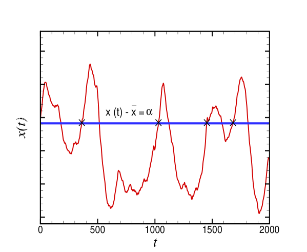
For the sake of clarity, we begin with a summary of the LC analysis rice44 ; newland ; Tabar1 ; Jafari ; tabar2 ; jensen . Consider a typical time series $\{x(t)\}$ and $n_{\alpha}^{+}$ denotes the number of positive difference crossings (upcrossings) at level $x(t)-\bar{x}=\alpha$ in time interval $T$ (see Fig. 1). The mean value of $n_{\alpha}^{+}$ for all time intervals be $N_{\alpha}^{+}(T)$ Tabar1 ,

$$N_{\alpha}^{+}(T)=\langle n_{\alpha}^{+}(T)\rangle,$$ (1)

here $\langle.\rangle$, represents ensemble average. For a homogeneous (stationary) process, the average number of upcrossings is proportional to the time interval $T$. Subsequently,

$$N_{\alpha}^{+}(T)=\nu^{+}_{\alpha}T,$$ (2)

in which $\nu_{\alpha}^{+}$ is the average frequency of upcrossings at the level equates to $y=x(t)-\bar{x}=\alpha$. The frequency parameter $\nu_{\alpha}^{+}$ could be deduced from the underlying joint probability distributions of $y\equiv x(t)-\bar{x}$ and $y^{\prime}=\frac{y(t+\Delta t)-y(t)}{\Delta t}=\frac{\Delta y}{\Delta t}$, namely $p(y,y^{\prime})$ rice44 ; newland ; Tabar1 ; Jafari ; tabar2 . To this end, consider a time scale $\Delta t$ of a typical sample function, if $x(t)-\bar{x}<\alpha$ at time $t$ and $x(t)-\bar{x}>\alpha$ at $t+\Delta t$ or alternatively the changes in $x(t)$ is positive in the time interval $\Delta t$, there will be a positive crossing of $x(t)-\bar{x}=\alpha$. In an other word, two following necessary and sufficient conditions should be satisfied to have an upcrossing in time interval, $\Delta t$

$$x(t)-\bar{x} < \alpha\hskip 17.07182pt$$ (3)

$$\hskip 17.07182pt\frac{\Delta\left[x(t)-\bar{x}\right]}{\Delta t} > \frac{\alpha-\left[x(t)-\bar{x}\right]}{\Delta t}.$$

Figure 3: Time series of three fractional Gaussian noises with Hurst exponents $H$, $0.2,0.5$ and $0.8$ from up to down.

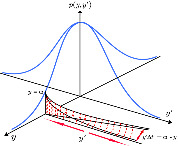
In order to examine whether the above conditions are satisfied at any arbitrary time $t$, we should find how the values of $y\equiv x(t)-\bar{x}$ and corresponding time derivative are distributed by considering their joint probability density $p(y,{y}^{\prime})$. Suppose that the level $y=\alpha$ and interval $\Delta t$ are specified. Then, we are only interested in values of $y<\alpha$ and values of ${y}^{\prime}>\frac{\alpha-y}{\Delta t}$, corresponding the region between the lines $y\leq\alpha$ and ${y}^{\prime}\geq\frac{\alpha-y}{\Delta t}$ in the plane of ($y,{y}^{\prime}$) (see Fig. 2). Therefore, the probability of positive slope crossing of $y=\alpha$ in $\Delta t$ is

$$\sum_{0}^{\infty}\Delta{y}^{\prime}\sum_{\alpha-{y}^{\prime}\Delta t}^{\alpha}\Delta yp(y,{y}^{\prime}).$$ (4)

We can replace $y$ with $\alpha$ when $\Delta t\rightarrow 0$

$$p(y,{y}^{\prime})=p(y=\alpha,{y}^{\prime}).$$ (5)

Since at large values of $y$ and ${y}^{\prime}$ the probability density function approaches zero fast enough (see Fig. 2), consequently expression (4) may be written as newland ; Tabar1

$$\int_{0}^{\infty}d{y}^{\prime}\int_{\alpha-{y}^{\prime}dt}^{\alpha}dyp(y=\alpha,{y}^{\prime})$$ (6)

in which the integrand is no longer as a function of $y$ so that the first integral is just $\int_{\alpha-{y}^{\prime}dt}^{\alpha}dyp(y=\alpha,{y}^{\prime})=p(y=\alpha,{y}^{\prime}){y}^{\prime}dt$. Finally the probability of upcrossing ($\nu_{\alpha}^{+}$) of $y=\alpha$ is equal to newland ; Tabar1

$$\nu_{\alpha}^{+}=\int_{0}^{\infty}p(\alpha,{y}^{\prime}){y}^{\prime}d{y}^{\prime}$$ (7)

in which the term $p(\alpha,{y}^{\prime})$ is the joint probability density $p(y,{y}^{\prime})$ evaluated at $y=\alpha$.

The integration of the Eq. (7) over all levels demonstrates another quantity, $N_{tot}^{+}$, which shows the total number of upcrossings for the data.

$$N_{tot}^{+}=\int_{-\infty}^{+\infty}\nu_{\alpha}^{+}d\alpha,$$ (8)

To study the effects of correlations or memory, $N_{sh}^{+}$ is evaluated which gives the total number of upcrossings of time series when it is shuffled. Here, random permutation is used for shuffling the data. The autocorrelations are destroyed by the shuffling procedure. Hence, by comparing $N_{tot}^{+}$ of the original data with that of computed for shuffled data set, $N_{sh}^{+}$, we can obtain the magnitude of correlations in the time series and this gives useful information about the time series. In order to study the effect of distribution function in the data with non-Gaussian distribution function, the so-called surrogate procedure can be applied. In the surrogate method, the discrete Fourier transform (DFT) of the observed time series data is computed and then the phases of each complex amplitude of the DFT are replaced with independently distributed artificial uniform $(-\pi,+\pi)$ variates the92 ; Ashkenazy . The altered DFT is then inverse Fourier transformed to generate a surrogate time series. The correlations in the surrogate series could be kept unchanged (for more detail see appendix (B) reference leila ), but the probability function changes to a Gaussian distribution leila ; sc00 ; the92 ; the93 ; the97 ; mahsa . To obtain information about the effect of the phase randomization procedure on the PDF, one can also check the results of this procedure on the magnitude and sign series Ashkenazy . For the surrogate time series, $N_{su}^{+}$ can be calculated which is the total number of upcrossings of this time series.

Figure 4: Left panel) Positive level crossings (upcrossings) of different fractional Gaussian noises. The average values of all fGns have been shifted to zero and their standard deviations are one. Right panel) $N^{+}_{tot}$ of different fGns with respect to Hurst exponent. Symbols are given by numerical analysis and fitting function is given by Eq. (9).

Figure 5: Schematic comparison of positive level crossings for three fGns and their shuffled.

Figure 6: The relative difference, $\mathcal{R}$, as a function of $H$. Symbols are given by numerical analysis and the solid line corresponds to the fitting function which is given by Eq. (12).

III discussion and results

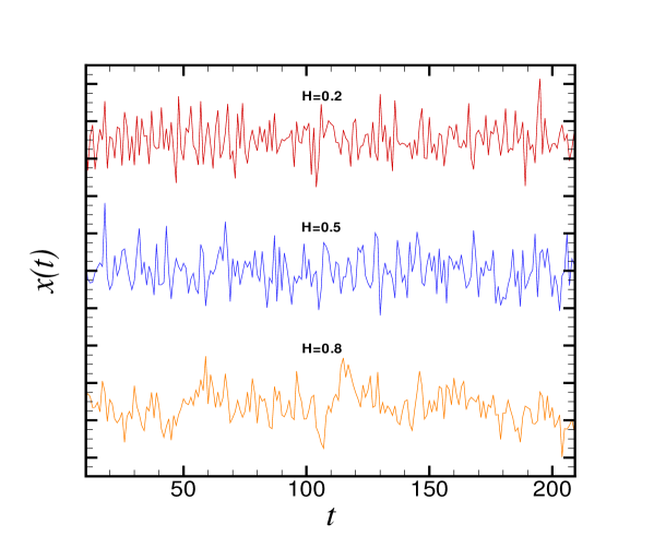
By using the PDF and the correlation function of the data, a stationary series can be pictured. Fractional Gaussian noises which are generalization of ordinary discrete white Gaussian noise are characterized by their Hurst exponent. Hurst exponent, H, gives a quantitative measure of the long-term persistence of a signal. In particular, the exponents $0<H<0.5$ and $0.5<H<1$ correspond to negative (anti-correlation) and positive correlation, respectively, while $H=0.5$ corresponds to an uncorrelated Gaussian process. For clarifying the level crossing results of unknown empirical data, their comparison with the results of well known fGns is emphasized. Fractional Gaussian noises can be generated using different methods Saupe ; Havlin ; Prakash ; Sahimi ; Pang ; Makse ; Mehrabi ; Voss ; Ausloos1 . Here, we have used the Fourier filtering method which was fully described in Refs. Saupe ; Havlin ; Prakash . In this method, the Fourier components of an uncorrelated sequence of random numbers are filtered by a suitable power-law filter in order to introduce correlations among the variables. In Fig. 3, we have plotted schematically three fractional Gaussian noises which are from up to down anticorrelated, random and correlated Gaussian noises. For a better comparison, their plots have been shifted vertically.

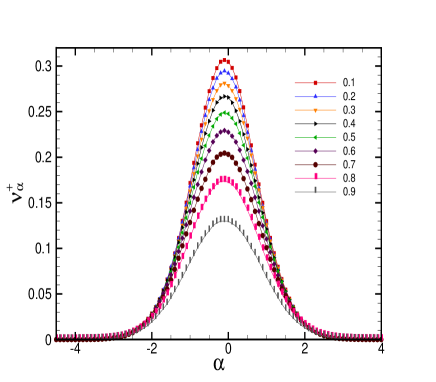
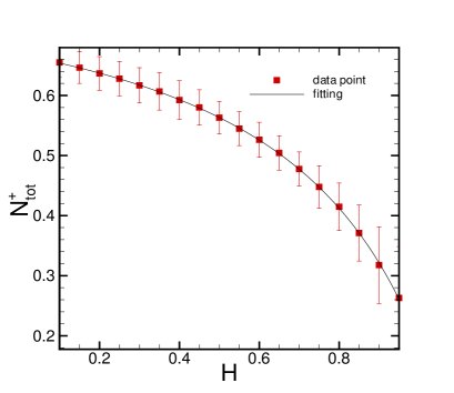
Level crossing function, $\nu^{+}_{\alpha}$, is calculated for different fractional Gaussian noises, according to Eq. 7. Fig. (4) (left panel) shows $\nu^{+}_{\alpha}$ as a function of level $\alpha$ for different values of Hurst exponent. By increasing the Hurst exponent of the fractional Gaussian noises the total number of upcrossings decreases (see Fig. (4) (right panel)). The behavior of the $N^{+}_{tot}$ elucidates the fact that by increasing the Hurst exponent the fluctuation in the time series decreases. The solid line shown in Fig. (4) (right panel) corresponds to a rational function of the following form that has been fitted to the curve of this figure with the goodness of fit equals to $r=0.999$.

$$N^{+}_{tot}=\frac{0.668-0.615H}{1-0.726H+0.012H^{2}}.$$ (9)

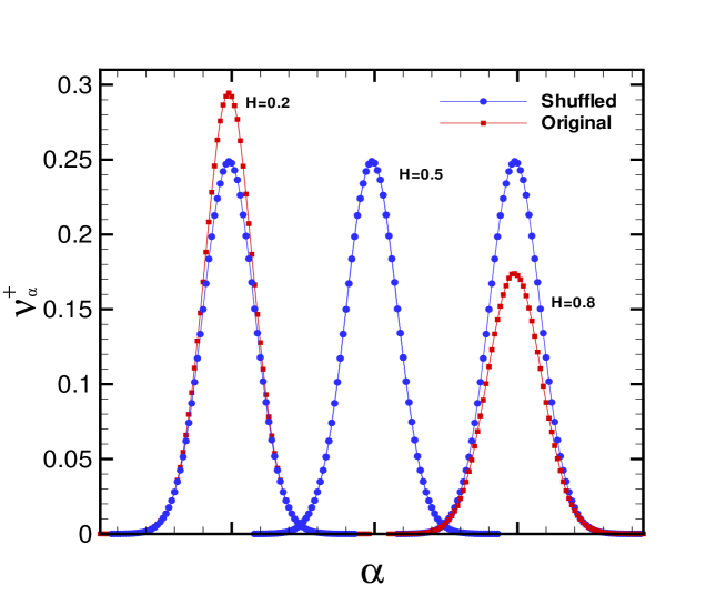
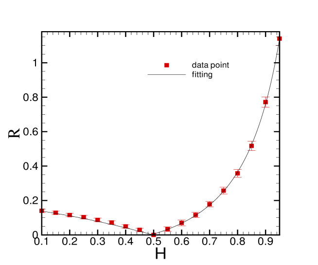
Now it is interesting to separate the correlation and the PDF effects by shuffling and surrogate procedures. These procedures are used in the level crossing method to elucidate its sensitivity to memory and PDF tabar2 ; mahsa . Since the PDF of the fractional Gaussian noise is the normal distribution, there is no more information in the surrogate method. By using the shuffling procedure, we can evaluate the memory of the series. In the case of fractional Gaussian noises, the total upcrossings (downcrossings) of the shuffled time series is increased for the correlated time series ($H>0.5$) while this behavior is reversed for the anticorrelated ones (see Fig. (5)). For the white noise, there is no change in the total positive level crossings because there is no correlation in the time series. For a better comparison, their plots have been shifted horizontally. By comparing the difference between $N^{+}_{tot}$ and $N^{+}_{sh}$ (after shuffling), the memory of the time series can be determined. Smaller relative difference denotes that the time series is less correlated (anticorrelated). As it is seen (Fig. (5)) under shuffling procedure the total positive level crossings $N^{+}_{tot}$, is increased (decreased) and this confirms that the underlying data set is correlated (anticorrelated). In order to quantify the value of memory (correlation and anticorrelation) embedded in the date set, we define the relative change of the total number of upcrossings by using the $N^{+}_{tot}$ for original and shuffled series as $\mathcal{R}\equiv|N_{sh}^{+}-N_{tot}^{+}|/N_{tot}^{+}$. In Fig. (6), $\mathcal{R}$ has been plotted for various values of Hurst exponents for different Hurst exponents. Two typical functions have been fitted to the curve of this figure which are

$$\mathcal{R}=\left\{\begin{array}[]{cc}\frac{0.161-0.323H}{1-0.744H-0.441H^{2}}&\ \ \ \ \ \ \ 0<H<0.5\\ \frac{-0.094+0.192H}{1-1.446H+0.500H^{2}}&\ \ \ \ \ \ \ 0.5<H<1\end{array}\right.$$ (12)

with the goodness of fit $r=0.999$ for each of them.

The probability density function of stationary empirical data set can be deviated from the Gaussian shape, consequently the total upcrossings of the so-called surrogate data is a relevant quantity to make our analysis complemented. In order to demonstrate, how $\mathcal{R}$ and the other defined parameters works, we applied this method to log-returns of three time series of financial markets which are $S\&P500$, Dow Jones and TSE. The results are reported in table 1. For better comparison, we have presented the results for a white noise. Here, we have used both the shuffling and surrogate procedures. As seen in the table, for shuffling procedure there is not that much change in the total positive level crossing for the two first markets which are considered as efficient markets. But, the shuffling procedure has strong effect on TSE which is an inefficient market. When the surrogate procedure is applied, the total positive level crossing for $S\&P500$ is not that much affected but for Dow Jones and TSE this is not the case. This is because their probability density functions are deviated from the Gaussian function. In order for them to be comparable to the fGns, they should be first surrogated. In fact, correlation and PDF both affect the level crossing method. Here, by using both of these procedures we want to consider both their effects.

Table 1: Total positive level crossings of the log-returns of three time series of financial markets ($S\&P500$, Dow Jones and TSE) for the original, shuffled and surrogated time series, and the relative difference of the shuffled and the original series one with its own pdf and the other when the pdf has been changed to a Gaussian. For better comparison these parameters are also presented for a white noise.

Index	$H$	$N^{+}_{tot}$	$N^{+}_{sh}$	$N^{+}_{su}$	$|N_{sh}^{+}-N_{tot}^{+}|/N_{tot}^{+}$	$|N_{su}^{+}-N_{tot}^{+}|/N_{tot}^{+}$
$S\&P500$	0.45	0.49	0.51	0.57	0.03	0.16
$Dow$ $Jones$	0.53	0.40	0.43	0.57	0.08	0.43
$TSE$	0.71	0.29	0.49	0.46	0.66	0.59
$White$ $noise$	0.5	0.56	0.56	0.56	0.00	0.00

IV Conclusion

Level crossing method with no required scaling feature is a powerful method in characterizing the time series. This method not only introduces roughness in a new concept but also contains information about waiting time (the time interval to observe an event again, statistically). It can also measure the memory and non-Gaussianity. Besides all these inferences, there was lack of a suitable measure for better understanding the level crossing results of unknown empirical data. Fractional Gaussian noises with normal distributions which can be indicated by only a Hurst exponent are known samples that could play the role of this criterion. They can fill this vacancy by comparing their level crossing results with the results of the unknown empirical Data. In this article, the level crossing results of fGns are investigated. The deviation of the empirical data results form the fGn with the same Hurst exponent is a measure of correlation and non-Gaussianity in the empirical one.

References

- (1) S.O. Rice, Mathematical Analysis of Random Noise, Bell System Tech. J. 23 (1944) 282; Mathematical Analysis of Random Noise, Bell System Tech. J. 24 (1945) 46.
- (2) D. E. Newland, An introduction to random vibrations, spectral and wavelet analysis, Longman Scientific & Technical, Third edition 1993.
- (3) F. Shahbazi, S. Sobhanian, M. Reza Rahimi Tabar, S. Khorram, G. R. Frootan, and H. Zahed, J. Phys. A 36, 2517 (2003).
- (4) M. Vahabi, G. R. Jafari, Chapter of Global Privatization and Its Impact, (Nova Science Publishers, 2009).
- (5) F. Ghasemi, M. Sahimi, J. Peinke, R. Friedrich, G. R. Jafari and M. Reza Rahimi Tabar, Phys. Rev. E 75, 060102(R) (2007).
- (6) M. H. Jensen, A. Johansen, F. Petroni, I. Simonsen, Physica A 340, 678 (2004); H. Ebadi, Meysam Bolgorian, G. R. Jafari, Physica A 389, 5530 (2010).
- (7) G. R. Jafari, M. S. Movahed, S. M. Fazeli, M. R. Rahimi Tabar, J. Stat. Mech. P06008 (2006).
- (8) I. Simonsen, M. H. Jensen and A. Johansen, Eur. Phys. J. B 27, 583 (2002); M. H. Jensen, A. Johansen and I. Simonsen, Physica A 234, 338 (2003).
- (9) A. Bunde, J. F. Eichner, J. W. Kantelhardt, and Sh. Havlin, Phys. Rev. Lett. 94, 048701 (2005).
- (10) G. F. Newell and M. Rosenblatt in Ann. Math. Statist. 33, 1306 (1962).
- (11) M. Vahabi, G. R. Jafari, Physica A 385, 583 (2007); M. Vahabi and G. R. Jafari, Physica A 388, 3859 (2009).
- (12) Yahoo finance; Tehran Stock Exchange, www.tse.ir
- (13) M. Sadegh Movahed and Shahram Khosravi, JCAP03 (2011) 012.
- (14) J. Theiler, S. Eubank, A. Longtin, B. Galdrikian, J. D. Farmer, Physica D 58, 77 (1992).
- (15) Y. Ashkenazy, P. Ch. Ivanov, Sh. Havlin, C-K. Peng, A. L. Goldberger, and H. E. Stanley, Phys. Rev. Lett. 86, 1900 (2001).
- (16) L. Hedayatifar, M. Vahabi, G. R. Jafari, Phys. Rev. E 84, 021138 (2011).
- (17) Thomas Schreiber and Andreas Schmitz, Physica D 142, 346 (2000).
- (18) J. Theiler, P. S. Linsay, and D. M. Rubin, Time Series Prediction: Forecasting the Future and Understanding the Past, A. S. Weigend and N. A. Gershenfeld, Proc. Vol. XVII, (Addison-Wesley, 1993).
- (19) J. Theiler, D. Prichard, Fields Inst. Commun. 11, 99 (1997).
- (20) D. Saupe, The Science of Fractal Images, edited by H.-O. Peitgen and D. Saupe (Springer, New York, 1988); J. Feder, Fractals (Plenum Press, New York, 1988).
- (21) C. -K. Peng, S. Havlin, M. Schwartz, H. E. Stanley, Phys. Rev. A 44, R2239 (1991).
- (22) S. Prakash, S. Havlin, M. Schwartz, H. E. Stanley, Phys. Rev. A 46, R1724 (1992).
- (23) H. Hamzehpour, and M. Sahimi, Phys. Rev. E 73, 056121 (2006).
- (24) N. -N. Pang, Y. -K. Yu, T. Halpin-Healy, Phys. Rev. E 52, 3224 (1995).
- (25) H. A. Makse, S. Havlin, M. Schwartz, and H. E. Stanley, Phys. Rev. E 53, 5445 (1996).
- (26) A. R. Mehrabi, H. Rassamdana, and M. Sahimi, Phys. Rev. E 56, 712 (1997).
- (27) R. F. Voss, Fundamental Algorithms for Computer Graphics, edited by R. A. Earnshaw, NATO ASI Series, Vol. 17 (Springer-Verlag, Heidelberg, 1985), p. 805; S. Lu, F. J. Molz, and H.-H. Liu, Comput. Geosci. 29, 15 (2003).
- (28) M. Ausloos and D. H. Berman, Proc. R. Soc. London, Ser. A 400, 331 (1985); W. Yan and K. Komvopoulos, J. Appl. Phys. 84, 3617 (1998).