On the nonlocal viscosity kernel of mixtures

Abstract

In this report we investigate the multiscale hydrodynamical response of a liquid as a function of mixture composition. This is done via a series of molecular dynamics simulations where the wave vector dependent viscosity kernel is computed for three mixtures each with 7-15 different compositions. We observe that the nonlocal viscosity kernel is dependent on composition for simple atomic mixtures for all the wave vectors studied here, however, for a model polymer melt mixture the kernel is independent of composition for large wave vectors. The deviation from ideal mixing is also studied. Here it is shown that a Lennard-Jones mixture follows the ideal mixing rule surprisingly well for a large range of wave vectors, whereas for both the Kob-Andersen mixture and the polymer melt large deviations are found. Furthermore, for the polymer melt the deviation is wave vector dependent such that there exists a critical length scale at which the ideal mixing goes from under-estimating to over-estimating the viscosity.

Hydrodynamics on very small length scales has become an important research area because it is believed to hold the key to understand the many new phenomena observed in nanofluidic devices. Recent studies Todd et al. (2008); Todd and Hansen (2008) have shown that the spatial correlations in the fluid reduce the shear stress compared to the stress predicted via a local response function. The nonlocal response is described via generalized hydrodynamics Alley and Alder (1983), in which the response function is a wave vector dependent quantity. The wave vector dependent viscosity, i.e. the viscosity kernel, accounts for the momentum flux due to nonzero strain rate. It has been found for one component fluids through molecular dynamics simulations and it was found that it follows a simple functional form reasonably well for atomic, diatomic and polymer fluids Alley and Alder (1983); Hansen et al. (2007); Puscasu et al. (2010a, b). By now the effect of the multiscale response is understood fairly well for a range of simple single component fluids Alley and Alder (1983); Hansen et al. (2007); Puscasu et al. (2010a, b) and glasses Furukawa and Tanaka (2009); Puscasu et al. (2010c).

In order to investigate the multiscale hydrodynamical response as a function of composition, we here evaluate the viscosity kernel for three different two component mixtures using molecular dynamics. In details, these are (i) a Kob-Andersen (KA) mixture Kob and Andersen (1994), (ii) a Lennard-Jones (LJ) mixture using the Lorentz-Berthelot mixing rule, and (iii) a model polymer melt mixture Kremer and Grest (1990). In all the simulations the particles interact through the Lennard-Jones cut and shifted potential $U_{LJ}(r_{ij})=4\epsilon\left[\left(\sigma/r_{ij}\right)^{12}-\left(\sigma/r_{ij}\right)^{6}\right]-U(r_{c})$ for $r_{ij}\leq r_{c}$, where $r_{ij}$ is the distance between particle $i$ and $j$, $\sigma$ is a length scale, $\epsilon$ is an energy scale, $r_{c}$ is the interaction range (cut-off) and $U(r_{c})$ is the unshifted potential at $r_{c}$. The values of $\sigma$ and $\epsilon$ are different for the KA and LJ mixtures depending on the pair of particles that interact, see Table 1.

	Kob-Andersen	Lennard-Jones
$\epsilon_{AA}/\epsilon_{AA}$	1	1
$\epsilon_{BB}/\epsilon_{AA}$	1/2	1/2
$\epsilon_{AB}/\epsilon_{AA}$	0.8	$\sqrt{1/2}$
$\sigma_{AA}/\sigma_{AA}$	1	1
$\sigma_{BB}/\sigma_{AA}$	0.88	0.88
$\sigma_{AB}/\sigma_{AA}$	0.8	0.94

Table 1: List of the Kob-Andersen and Lennard-Jones parameters used in this work.

The cut-off radius is set to $r_{c}=2.5\sigma$ for the KA and LJ mixtures and $r_{c}=2^{1/6}\sigma$ for the polymer melt. The latter is also referred to as the Weeks-Chandler-Andersen pair potential Weeks et al. (1971). In the polymer melt the particles (or beads) are bonded via the Finite Extensible Nonlinear Elastic (FENE) potential Kremer and Grest (1990) $U_{FENE}=-kR_{0}\ln\left[1-\left(r_{ij}/R_{0}\right)^{2}\right]/2$, where $k=30\epsilon/\sigma^{2}$ and $R_{0}=1.5\sigma$. The polymer melt is composed of two types of molecules, one with two beads, component B, and one with ten beads, component A. In what follows we give all quantities in terms of Lennard-Jones reduced units, for example, reduced distance $r_{ij}^{*}=r_{ij}/\sigma$ and number density $\rho^{*}=\rho\sigma^{3}$. For simplicity of notation, we will hereafter omit the asterisk.

The simulations are carried out at an average reduced pressure of $p=1$ and temperature $T=2.5$. The target pressure was obtained via an anisotropic Berendsen barostat Berendsen et al. (1984) such the simulation box was extended in the $x$ direction only. The temperature was controlled via a Nosé-Hoover thermostat Nosé (1984); Hoover (1985).

The expression for the wave vector dependent viscosity can be found from the generalized Navier-Stokes equation and is given in terms of the transverse momentum current density autocorrelation function $\widetilde{C}_{\perp}(k,t)$ Hansen and McDonald (2006); Palmer (1994)

$$\eta(k,\omega)=\frac{\widetilde{C}_{\perp}(k,t=0)-i\omega\widehat{C}_{\perp}(k,\omega)}{\widehat{C}_{\perp}(k,\omega)k^{2}/\rho}\ ,$$ (1)

where $\rho$ is the mass density, $k$ is the $z$ component the wave vector, i.e.

$$k=2\pi n/L_{z}\ ,\ \ \ n=1,2,\ldots\ ,$$ (2)

where $L_{z}$ is the simulation box length in the $z$ direction, and $\widetilde{C}_{\perp}(k,t)=\langle\widetilde{J}_{y}(k,0)\widetilde{J}_{y}(k,t)\rangle/V$. The transverse momentum density is here defined via $\widetilde{J}_{y}(k,t)=\sum_{i=1}^{N}m_{i}v_{y}(t)e^{ikz},$ where $m_{i}$ and $v_{y}$ are the center of mass and center of mass velocity of molecule or particle $i$. We note that $\widehat{C}_{\perp}(k,\omega)$ is the Fourier-Laplace transform of $\widetilde{C}_{\perp}(k,t)$, that is, $\widehat{C}_{\perp}(k,\omega)=\int_{0}^{\infty}\widetilde{C}_{\perp}(k,t)e^{i\omega t}dt$. Also note, because the barostat is anisotropic and only varies the simulation box in the $x$ direction $L_{z}$ is constant in Eq.(2).

In Fig. 1 we have plotted the viscosity kernel data in the limit $\omega\rightarrow 0$ for different composition fractions of A, $x_{A}=N_{A}/N_{t}$ where $N_{A}$ is the number of A particles and $N_{t}$ is the total number of particles.

Figure 1: Viscosity kernel data (symbols) for the Kob-Andersen mixture (a), the Lennard-Jones mixture (b) and the polymer mixture (c). In (a) and (b): $x_{A}=0$ (filled squares), 0.8 (upwards pointing triangles), and 1 (downwards pointing triangles). In (c): $x_{A}=0$ (filled squares), 0.25 (upwards pointing triangles) and 1 (downwards pointing triangles). The error bars are the standard error. Lines represent the best fit of the data to Eq. (3). The inset windows depict the kernels for large $k$.

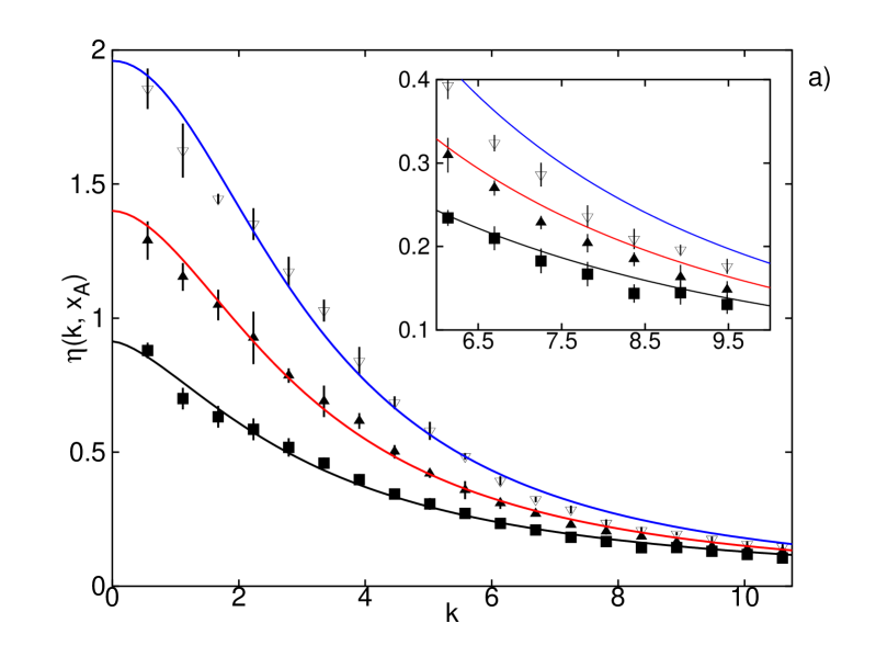
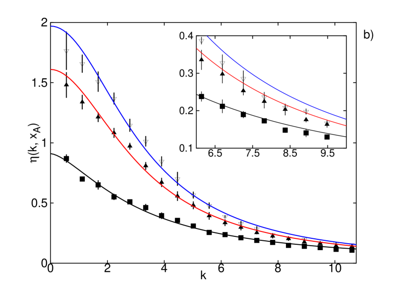
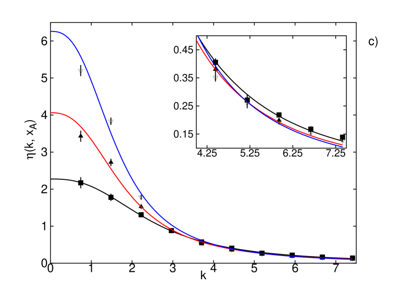
Recall, that in the polymer melt we denote the 10 bead polymer A. From Fig. 1 it is observed that for the KA and LJ mixtures the hydrodynamical response is dependent on the exact composition for all length scales studied here. This is not the case for the polymer mixture: here the fluid response is largely independent of the fluid composition for sufficiently large wave vectors. In order to decrease the statistical error in the further analysis we fit the data to a Lorentzian functional form

$$\eta(k,x_{A})=\frac{\eta_{0}(x_{A})}{1+\alpha k^{\beta}}\ ,$$ (3)

where $\alpha$ and $\beta$ are fitting parameters that depend on the fraction of A, $x_{A}$, and $\eta_{0}(x_{A})$ is the zero frequency viscosity for $k=0$. Eq. (3) has been shown to fit viscosity kernel data well for a range of different non-charged single component fluids Hansen et al. (2007); Puscasu et al. (2010a, b). The result of the fitting is also depicted in Fig. 1 where the inset windows show the data and the fits for large values of $k$. It is seen that Eq. (3) fits data well for all three systems, however, we stress that the agreement is not satisfactory for large values of $k$ in the cases of Kob-Andersen and Lennard-Jones mixtures. With this in mind we, will from now on use the fitted values of the viscosity kernels rather than the raw MD data.

We can define the $k$ dependent excess viscosity as

$$\eta^{E}(k,x_{A})=\eta(k,x_{A})-\eta^{\text{id}}(k,x_{A})\ ,$$ (4)

where $\eta^{\text{id}}(k,x_{A})$ is the ideal part of the viscosity kernel given by an Arrhenius type mixing rule Arrhenius (1887); Kendall and Monroe (1921)

$$\eta^{\text{id}}(k,x_{A})=\eta_{A}(k)^{x_{A}}\eta_{B}(k)^{1-x_{A}}$$ (5)

Here $\eta_{A}(k)$ and $\eta_{B}(k)$ are the viscosity kernels of pure $A$ and $B$, respectively. The excess viscosity has been fitted to various simple mixing models including the Kendall-Monroe model Kendall and Monroe (1921), the Lederer model, see for example Ref. Lederer (1931), and an extended version of the Grundberg-Nissan model Grundberg and Nissan (1949). We have found that the fourth order McAllister model McAllister (1960) fitted the data best. This model is originally written in terms of the dynamical viscosity $\nu=\eta/\rho$ and may readily be extended to include the wave vector dependency, that is,

$$\ln\nu(k,x_{A}) = x_{A}^{4}\ln[\nu_{A}(k)]+4x_{A}^{3}x_{B}\ln[M_{31}(k)]+6x_{A}^{2}x_{B}^{2}\ln[M_{22}(k)]+$$ (6)

$$4x_{A}x_{B}^{3}\ln[M_{13}(k)]+x_{B}^{4}\ln[\nu_{B}(k)]-\ln(x_{A}+x_{B}m_{r})+$$

$$4x_{A}^{3}x_{B}\ln\left(\frac{3+m_{r}}{4}\right)+6x_{A}^{2}x_{B}^{2}\ln\left(\frac{1+m_{r}}{2}\right)+$$

$$4x_{A}x_{B}^{3}\ln\left(\frac{1+3m_{r}}{4}\right)+x_{B}^{4}\ln(m_{r})\ ,$$

where $m_{r}$ is given by $m_{B}/m_{A}$ and $M_{31},M_{22}$ and $M_{13}$ are the wave vector dependent McAllister coefficients. Recall, since we study binary mixtures $x_{B}=1-x_{A}$. From Eq. (6) one can easily extract the McAllister excess kinematic viscosity using $M_{31},M_{22}$ and $M_{13}$ as fitting parameters Rather than comparing the absolute excess viscosities, we compare the relative deviation from ideal mixing using $\eta^{E}(k,x_{A})/\eta(k,x_{A})=1-\eta^{\text{id}}(k,x_{A})/\eta(k,x_{A})$. This is done in Fig. 2.

Figure 2: Relative excess viscosity as function of composition and wave number, $n$. a) The Kob-Andersen mixture, b) the Lennard-Jones mixture and c) the polymer mixture. Full li nes are the corresponding fits using Eqs. (6) and (5).

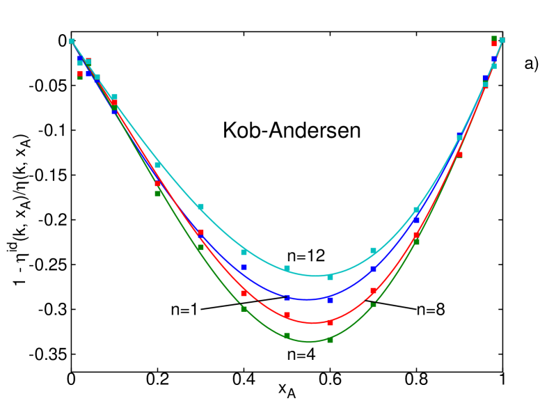
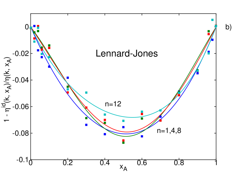
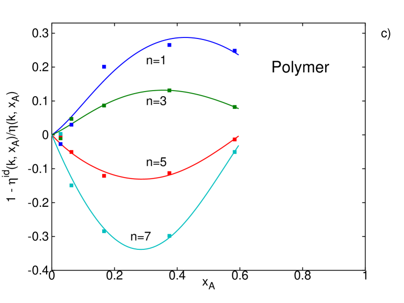
We also note that the normalized excess viscosity is a measure of the relative deviation from ideal mixing. Firstly, it is observed that the KA and polymer mixtures feature large deviations from the ideal mixing rule compared to the LJ mixture, that is, the Lorentz-Berthelot mixing rule features a more Arrhenius-like behavior compared to the KA mixing rule for all wave lengths. Secondly, for the KA and LJ mixtures the relative excess viscosity varies very little with respect to wave vector meaning that the relative difference between the ideal mixing response function and the actual response is weakly wave vector dependent. For the polymer mixture, Fig. 2 c), we observe that the relative excess viscosity is strongly wave vector dependent. This is also indicated in Fig. 1 c) where it was observed that the kernel is independent of composition for large $k$, but not for small $k$. This complex wave vector dependency means that there exists a critical length scale $l_{c}$ at which the ideal mixing term goes from under-estimating to over-estimating the viscosity. For the melt studied here it happens around $l_{c}=1.7$. This behavior indicates that for the polymer melt the local viscous response is independent of chain length at short wave lengths.

To discuss this special behavior further we have plotted the McAllister coefficients as functions of wave vector in Fig. 3.

Figure 3: McAllister coefficients as function of wave vector, $k$. Filled squares represent the results for the Kob-Andersen mixture, upward pointing triangles the Lennard-Jones mixture and downward pointing triangles the polymer mixture. Lines serve as a guide to the eye.

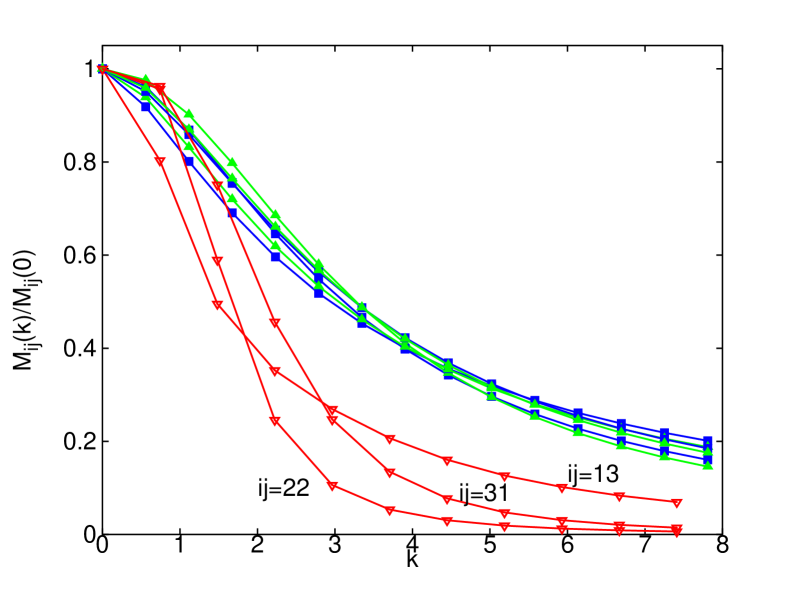
We see that $M_{ij}(k)/M_{ij}(0),\{ij\}=\{31\},\{22\}$ and $\{13\}$, fall on a master curve in the case of KA and LJ mixtures. This means that the three functions, $M_{ij}(k)$, may be described by a single master function which is directly proportional to any of the three $M_{ij}(k)$. For the polymer mixture, on the other hand, this is not the case. Note, that all the McAllister coefficients follow a Lorentzian form, see Eq. (3), but for the polymer mixture the parameters $\alpha$ and $\beta$ are dependent on the index $\{ij\}$.

In this report we have investigated the multiscale hydrodynamical viscous response as a function of fluid composition. This was done through the viscosity kernel that was computed via equilibrium molecular dynamics simulations. We studied three different mixtures, namely, (i)a Kob-Andersen mixture, (ii) a Lennard-Jones mixture using Lorentz-Berthelot mixing rule, and (iii) a polymer melt mixture. We observed that the viscosity kernel is independent of the wave vector for large wave vectors in the case of a polymer melt, that is, the hydrodynamical response at these length scales is independent of the composition. This was not the case for the simple Kob-Andersen and Lennard-Jones mixtures. The deviation from ideal mixing is low in the case of the Lennard-Jones mixture, i.e. the Lorentz-Berthelot mixing rule agrees reasonably well with the predictions from ideal mixing for all wave vectors studied here. This is not the case for Kob-Andersen and polymer mixtures. Finally, the relative deviation from ideal mixing is relatively wave vector independent in the case of the Kob-Andersen and Lennard-Jones mixtures. However, for the polymer mixture this deviation shows a strong wave vector dependency, since the ideal mixing rule does not predict the largely wave vector independent behavior of the kernel, Fig 1 c).

J.S. Hansen wishes to acknowedge Lundbeckfonden for supporting this work as a part of Grant No. R49-A5634. The authors also wishes to thank Prof. Peter J. Daivis for useful comments.

References

- Todd et al. (2008) B. D. Todd, J. S. Hansen, and P. Daivis, Phys. Rev. Lett. 100, 195901 (2008).
- Todd and Hansen (2008) B. D. Todd and J. S. Hansen, Phys.Rev.E 78, 051702 (2008).
- Alley and Alder (1983) W. E. Alley and B. J. Alder, Phys. Rev. A 27, 3158 (1983).
- Hansen et al. (2007) J. S. Hansen, P. J. Daivis, K. P. Travis, and B. D. Todd, Phys. Rev. E 76, 041121 (2007).
- Puscasu et al. (2010a) R. Puscasu, B. Todd, P. J. Daivis, and J. Hansen, J. Phys.: Condens. Matter 22, 195105 (2010a).
- Puscasu et al. (2010b) R. Puscasu, B. Todd, P. J. Daivis, and J. Hansen, Phys. Rev. E 82, 011801 (2010b).
- Furukawa and Tanaka (2009) A. Furukawa and H. Tanaka, Phys. Rev. Lett. 103, 135703 (2009).
- Puscasu et al. (2010c) R. Puscasu, B. Todd, P. J. Daivis, and J. Hansen, J. Chem. Phys. 133, 144907 (2010c).
- Kob and Andersen (1994) W. Kob and H. Andersen, Phys. Rev.E 73, 1376 (1994).
- Kremer and Grest (1990) K. Kremer and G. S. Grest, J. Chem. Phys. 92, 5057 (1990).
- Weeks et al. (1971) J. D. Weeks, D. Chandler, and H. C. Andersen, J. Chem. Phys. 54, 5237 (1971).
- Berendsen et al. (1984) H. Berendsen, J. Postma, W. van Gunsteren, A. DiNola, and J. R. Haak, J. Chem. Phys. 81, 3684 (1984).
- Nosé (1984) S. Nosé, Mol. Phys. 52, 255 (1984).
- Hoover (1985) W. G. Hoover, Phys. Rev. A 31, 1695 (1985).
- Hansen and McDonald (2006) J. P. Hansen and I. R. McDonald, Theory of Simple Liquids (Academic Press, Amsterdam, 2006).
- Palmer (1994) P. Palmer, 49, 359 (1994).
- Arrhenius (1887) S. Arrhenius, Phys. Chem. 1, 285 (1887).
- Kendall and Monroe (1921) J. Kendall and K. Monroe, J. Am. Chem. Soc. 43, 115 (1921).
- Lederer (1931) E. Lederer, Nature 139, 27 (1931).
- Grundberg and Nissan (1949) L. Grundberg and A. Nissan, Nature 164, 799 (1949).
- McAllister (1960) R. McAllister, AIChE J. 6, 427 (1960).