Entanglement of two harmonic modes coupled by angular momentum

Abstract

We examine the entanglement induced by an angular momentum coupling between two harmonic systems. The Hamiltonian corresponds to that of a charged particle in a uniform magnetic field in an anisotropic quadratic potential, or equivalently, to that of a particle in a rotating quadratic potential. We analyze both the vacuum and thermal entanglement, obtaining analytic expressions for the entanglement entropy and negativity through the gaussian state formalism. It is shown that vacuum entanglement diverges at the edges of the dynamically stable sectors, increasing with the angular momentum and saturating for strong fields, whereas at finite temperature, entanglement is non-zero just within a finite field or frequency window and no longer diverges. Moreover, the limit temperature for entanglement is finite in the whole stable domain. The thermal behavior of the gaussian quantum discord and its difference with the negativity is also discussed.

I Introduction

The investigation of quantum entanglement and quantum correlations in distinct physical systems is of great interest for both quantum information and many-body physics NC.00 ; VE.07 ; AFOV.08 ; HHHH.10 . While the evaluation of entanglement in systems with a high dimensional Hilbert space is in general a difficult problem, boson systems described by quadratic Hamiltonians in the basic boson operators offer the invaluable advantage of admitting an exact evaluation of entanglement measures in both the ground and thermal state, through the gaussian state formalism RS.00 ; WW.01 ; AEPW.02 ; ASI.04 ; CEPD.06 ; AI.08 ; MRC.10 . The latter allows to express the entanglement entropy BBPS.96 and negativity ZHSL.99 ; VW.02 of any bipartition of a gaussian state in terms of the symplectic eigenvalues of covariance matrices of the basic operators. Moreover, the positive partial transpose (PPT) separability criterion PP.96 ; HHH.96 is both necessary and sufficient for two-mode mixed gaussian states RS.00 (and also $(1,n-1)$ bipartitions of $n$ modes gaussian states WW.01 ), turning the negativity into a rigorous entanglement indicator for these systems. Let us also remark that there is presently a great interest in continuous variable based quantum information BvL.05 , where gaussian states constitute the basic element.

In addition, an approximate yet analytic evaluation of the quantum discord OZ.01 ; HV.01 in two-mode gaussian states was recently achieved GP.10 ; AD.10 , by restricting the local measurement that determines this quantity to a gaussian measurement BvL.05 . Quantum discord is a measure of quantum correlations which coincides with the entanglement entropy in pure states but differs essentially from entanglement in mixed states, where it can be non-zero even if the state is separable, i.e., with no entanglement. The current interest in the quantum discord was triggered by its presence DSC.08 in certain mixed state based quantum computation schemes which provide exponential speedup over classical ones KL.98 , yet exhibiting no entanglement DFC.05 . Important properties of states with non-zero discord were recently unveiled CAB.11 ; SKD.11 ; PGA.11 .

The aim of this work is to examine, using the gaussian state formalism, the entanglement and quantum correlations between two harmonic modes generated by an angular momentum coupling. Such system arises, for instance, when considering a charged particle in a uniform magnetic field in an anisotropic quadratic potential, or also a particle in a rotating anisotropic harmonic trap Va.56 ; FK.70 ; RS.80 ; BR.86 . The model has then been employed in several areas, including the description of deformed rotating nuclei RS.80 ; BR.86 , anisotropic quantum dots in a magnetic field MC.94 , and fast rotating Bose-Einstein condensates LNF.01 ; OO.04 ; AF.07 ; ABL.09 in the lowest Landau level approximation ABD.05 ; BDS.08 ; AF.09 . Containing just quadratic couplings in the associated boson operators, the different terms in the Hamiltonian may in principle be also simulated by standard optical means BvL.05 ; PE.94 . For a general quadratic potential, the model exhibits a complex dynamical phase diagram RK.09 , presenting distinct types of stable and unstable domains and admitting the possibility of stabilizing an initially unstable system by increasing the field or frequency RK.09 . The model provides then an interesting and physically relevant scenario for analyzing the behavior of mode entanglement in different regimes and near the onset of different types of instabilities, with the advantage of allowing an exact analytic evaluation of entanglement and quantum correlation measures at both zero and finite temperature. In addition, the present results indicate that mode entanglement can be easily controlled in this systems by modifying the field or frequency, suggesting a potential for quantum information applications. Let us finally mention that the dynamics of entanglement in other two-mode systems were examined in HMM.03 ; NL.05 ; CN.08 .

In sec. II we describe the model and derive the analytic expressions for the vacuum entanglement entropy and the thermal negativity. The basic features of the quantum discord are also discussed. The detailed behavior of entanglement with the relevant control parameters is then analyzed in sec. III, where we show that while vacuum entanglement diverges at the edges of stable sectors, being correlated with the angular momentum, at finite temperature entanglement is finite, and non-zero just within a finite field window and below a finite limit temperature. A comparison between the thermal behavior of the negativity and that of the gaussian quantum discord is finally made, which indicates a quite different thermal response of these two quantities, with the discord vanishing only asymptotically for $T\rightarrow\infty$. Conclusions are finally drawn in IV.

II Formalism

II.1 Model Hamiltonian

We consider a system described by the Hamiltonian

$$H=\frac{1}{2}(P_{x}^{2}+k^{\prime}_{x}Q_{x}^{2})+\frac{1}{2}(P_{y}^{2}+k^{\prime}_{y}Q_{y}^{2})-\omega(Q_{x}P_{y}-Q_{y}P_{x})\,,$$ (1)

which represents two harmonic modes coupled by an angular momentum term. Here $Q_{\mu}$, $P_{\mu}$ stand for dimensionless coordinates and momenta ($[Q_{\mu},P_{\nu}]=i\delta_{\mu\nu}$, $[Q_{\mu},Q_{\nu}]=[P_{\mu},P_{\nu}]=0$). Eq. (1) arises, for instance, in the description of a particle of charge $e$ and mass $m$ in a general quadratic potential subject to a uniform magnetic field, parallel to a principal axis of the potential. Denoting this axis as $z$, such Hamiltonian reads

$${\cal H} = \frac{(\bm{P}-e\bm{A}/c)^{2}}{2m}+\frac{1}{2}(K_{x}{\cal Q}_{x}^{2}+K_{y}{\cal Q}_{y}^{2}+K_{z}{\cal Q}_{z}^{2})$$ (2)

$$= \frac{1}{2}[\frac{{\cal P}_{x}^{2}+{\cal P}^{2}_{y}}{m}+K^{\prime}_{x}{\cal Q}_{x}^{2}+K^{\prime}_{y}{\cal Q}_{y}^{2}-\Omega{\cal L}_{z}]+{\cal H}_{z}\,,$$ (3)

where $\mathbf{A}=\frac{1}{2}\bm{H}\times\bm{Q}$ is the vector potential, $\Omega=\frac{e|\mathbf{H}|}{mc}$ the cyclotron frequency, ${\cal L}_{z}={\cal Q}_{x}{\cal P}_{y}-{\cal Q}_{y}{\cal P}_{x}$, ${\cal H}_{z}=\frac{1}{2}(\frac{{\cal P}_{z}^{2}}{m}+K_{z}{\cal Q}_{z}^{2})$ and $K^{\prime}_{\mu}=K_{\mu}+m\Omega^{2}/4$. Eq. (3) is also identical with the intrinsic Hamiltonian of a particle of mass $m$ in a quadratic potential of constants $K^{\prime}_{\mu}$ rotating around the $z$ axis with frequency $\Omega/2$ RS.80 ; BR.86 .

The replacement ${\cal P}_{\mu}=P_{\mu}\sqrt{\hbar m\Omega_{0}}$, ${\cal Q_{\mu}}=Q_{\mu}/\sqrt{m\Omega_{0}/\hbar}$ in (3), with $\Omega_{0}$ a reference frequency, leads to ${\cal H}=\hbar\Omega_{0}H+{\cal H}_{z}$, with $H$ given by (1) and

$$k^{\prime}_{\mu}=k_{\mu}+\omega^{2}\,,\;\;k_{\mu}=\frac{K_{\mu}}{m\Omega_{0}^{2}}\,,\;\;\omega=\frac{\Omega}{2\Omega_{0}}\,.$$ (4)

We note that in terms of the boson operators $b_{\mu}=(Q_{\mu}+iP_{\mu})/\sqrt{2}$, the scaled angular momentum $L_{z}={\cal L}_{z}/\hbar$ in (1) is

$$L_{z}=Q_{x}P_{y}-Q_{y}P_{x}=-i(b^{\dagger}_{x}b_{y}-b^{\dagger}_{y}b_{x})\,,$$ (5)

and can then be simulated by standard linear optics, although for such bosons the first two terms in (1) become $\sum_{\mu=x,y}g_{\mu}^{+}(b^{\dagger}_{\mu}b_{\mu}+\frac{1}{2})+g_{\mu}^{-}(b_{\mu}^{2}+{b^{\dagger}_{\mu}}^{2})$, with $g_{\mu}^{\pm}=\frac{k^{\prime}_{\mu}\pm 1}{2}$, and require non-linear means. If $K^{\prime}_{x}>0$, we can set $k^{\prime}_{x}=1$, i.e., $g_{x}^{-}=0$, by adequately fixing $\Omega_{0}$ in (4), but $g_{y}^{-}$ remains non-zero in the relevant anisotropic case $k^{\prime}_{y}\neq k^{\prime}_{x}$, where $[H,L_{z}]\neq 0$. The change to normal $x,y$ bosons, such that $H=\sum_{\mu=x,y}\sqrt{k^{\prime}_{\mu}}(\tilde{b}^{\dagger}_{\mu}\tilde{b}_{\mu}+\frac{1}{2})-\omega L_{z}$, will lead instead to an additional term $\propto(1-\sqrt{\frac{k^{\prime}_{x}}{k^{\prime}_{y}}})(\tilde{b}_{x}\tilde{b}_{y}-\tilde{b}^{\dagger}_{x}\tilde{b}^{\dagger}_{y})$ in $L_{z}$.

II.2 Diagonalization and stability

If the parameter

$$\Delta=\sqrt{(k^{\prime}_{x}-k^{\prime}_{y})^{2}/4+2\omega^{2}(k^{\prime}_{x}+k^{\prime}_{y})}$$ (6)

is non-zero, the canonical transformation

$$P^{\prime}_{\mu} = P_{\mu}+\gamma Q_{-\mu}\,,\;\;\;\;Q^{\prime}_{\mu}=\frac{Q_{\mu}-\eta P_{-\mu}}{1+\eta\gamma}\,,$$ (7)

where $\gamma=\frac{2\Delta-k^{\prime}_{x}+k^{\prime}_{y}}{4\omega}$, $\eta=\frac{2\gamma}{k^{\prime}_{x}+k^{\prime}_{y}}$ and labels $(x,y)$ are now identified with $(+,-)$, allows to write Eq. (1) as RK.09

$$H = \sum_{\mu=\pm}\frac{1}{2}(\alpha_{\mu}{P^{\prime}}_{\mu}^{2}+\beta_{\mu}{Q^{\prime}}_{\mu}^{2})\,,$$ (8)

where $\alpha_{\pm}=1-{\textstyle\frac{\omega}{\Delta}}(\gamma\mp\omega)$ and $\beta_{\pm}={\textstyle\frac{\Delta}{\omega}}(\gamma\pm\omega)$. If $\Delta=0$ and $\omega\neq 0$, a separable representation of the form (8) in terms of canonical variables ($[Q^{\prime}_{\mu},P^{\prime}_{\nu}]=\delta_{\mu\nu}$, $[P^{\prime}_{\mu},P^{\prime}_{\nu}]=[Q^{\prime}_{\mu},Q^{\prime}_{\nu}]=0$) is not feasible. Such a possibility can arise in the repulsive case $k_{\mu}\leq 0$, when the $4\times 4$ matrix representing the quadratic form (1) is not diagonalizable with the symplectic metric and leads to non-trivial Jordan forms RK.09 .

For general real values of $k^{\prime}_{\mu}$ in (1), the coefficients $\alpha_{\mu}$, $\beta_{\mu}$ in (8) can be positive, zero, negative, and even complex RK.09 . We will here consider those cases where Eq. (8) can be further written as

$$H = \sum_{\mu=\pm}\lambda_{\mu}(b^{\prime\dagger}_{\mu}b^{\prime}_{\mu}+\frac{1}{2})\,,$$ (9)

$$|\lambda_{\pm}| = \sqrt{\alpha_{\pm}\beta_{\pm}}=\sqrt{{\textstyle\frac{k^{\prime}_{x}+k^{\prime}_{y}}{2}}+\omega^{2}\pm\Delta}\,,$$ (10)

with $\lambda_{\mu}$ real and ${b^{\prime}}_{\mu}=\sqrt{\frac{\beta_{\mu}}{2\lambda_{\mu}}}Q^{\prime}_{\mu}+i\sqrt{\frac{\alpha_{\mu}}{2\lambda_{\mu}}}P^{\prime}_{\mu}$ standard bosons ($[{b^{\prime}}_{\mu},{b^{\prime}}_{\nu}^{\dagger}]=\delta_{\mu\nu}$, $[{b^{\prime}}_{\mu},{b^{\prime}}_{\nu}]=[{b^{\prime}}^{\dagger}_{\mu},{b^{\prime}}^{\dagger}_{\nu}]=0$), such that $H$ exhibits a discrete spectrum. In these cases the matrix representing (1) is diagonalizable with the symplectic metric, with real symplectic eigenvalues RK.09 .

At fixed $k_{\mu}$ in (4) (charged particle in a magnetic field), Eq. (9) is valid in the following domains RK.09 (Fig. 1):
(A) $k_{x}>0$, $k_{y}>0$, where $\alpha_{\pm}>0$, $\beta_{\pm}>0$ and $\lambda_{\pm}>0$. This is the standard case of an attractive quadratic potential, where $H$ is positive definite and hence fully stable.
(B) $k_{x}<0$, $k_{y}<0$, and

$$|\omega|>\omega_{c}={\textstyle\frac{\sqrt{-k_{x}}+\sqrt{-k_{y}}}{2}}\,,$$ (11)

where $\alpha_{+}>0$, $\beta_{+}>0$ but $\alpha_{-}<0$, $\beta_{-}<0$, implying $\lambda_{+}>0$ but $\lambda_{-}<0$ in (9). This is the case of a repulsive quadratic potential, where $H$ becomes equivalent to a standard plus an inverted oscillator if $|\omega|>\omega_{c}$: It has no minimum energy, but is dynamically stable, as the motion remains bounded RK.09 . The dynamics around a quadratic potential maximum can then be stabilized by a sufficiently strong field.
(C) $k_{x}=k_{y}=0$ and $\omega\neq 0$ (Landau case), where $\Delta=2\omega^{2}$, $\alpha_{+}=1$, $\beta_{+}=4\omega^{2}$ whereas $\alpha_{-}=\beta_{-}=0$, leading to $\lambda_{+}=2|\omega|$ and $\lambda_{-}=0$. Eq. (9) becomes a standard plus a vanishing oscillator. Here the final choice of $b^{\prime}_{-}$, ${b^{\prime}}_{-}^{\dagger}$ is not fixed, as $\lambda_{-}=0$. We will set $b^{\prime}_{-}=\sqrt{\omega}Q^{\prime}_{-}+iP^{\prime}_{-}/\sqrt{4\omega}$, according to the $k_{\mu}\rightarrow 0$ limit of the isotropic case $k_{x}=k_{y}=k$, where $\lambda_{\pm}=\sqrt{k^{\prime}}\pm\omega$, $\Delta=2\omega\sqrt{k^{\prime}}$, $\gamma=\sqrt{k^{\prime}}=1/\eta$, $\alpha_{\mu}=\frac{1}{2}\lambda_{\mu}/\sqrt{k^{\prime}}$, $\beta_{\mu}=2\lambda_{\mu}\sqrt{k^{\prime}}$ and $k^{\prime}=k+\omega^{2}$.

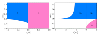
Figure 1: Left: Sectors with discrete spectrum at fixed $k_{\mu}$ (particle in a magnetic field plus quadratic potential) in the anisotropy-frequency plane $k_{y}/|k_{x}|,\omega/\omega_{0}$, where $\omega_{0}=\sqrt{|k_{x}|}$. $A$ is the positive definite sector, corresponding to an attractive potential $k_{\mu}>0$ for $\mu=x,y$, whereas $B$ the non-positive sector, corresponding to a repulsive potential $k_{\mu}<0$ for $\mu=x,y$ with $|\omega|>\omega_{c}$ (Eq. (11)). Right: Same sectors at fixed $k^{\prime}_{\mu}>0$ (particle in a rotating quadratic potential) in the $k^{\prime}_{y}/k^{\prime}_{x},\omega/\omega^{\prime}_{0}$ plane, where $\omega^{\prime}_{0}=\sqrt{k^{\prime}_{x}}$ and we have set $k^{\prime}_{x}>0$. $A$ is the positive definite sector (Eq. (12)), $B_{1}$ the non-positive sector with $k^{\prime}_{y}>0$ (Eq. (13)) and $B_{2}$ that with $k^{\prime}_{y}<0$ (Eqs. (14)–(15)). Quantities plotted in all figures are dimensionless.

At fixed $k^{\prime}_{\mu}$ in (1) (rotating potential), the previous sectors are seen quite differently. Sector (A) corresponds to $k^{\prime}_{x}>0$, $k^{\prime}_{y}>0$ and

$$|\omega|<\omega^{\prime}_{c1}={\rm Min}[\sqrt{k^{\prime}_{x}},\sqrt{k^{\prime}_{y}}]\,,$$ (12)

indicating a maximum allowable frequency in an attractive rotating quadratic potential (right panel in Fig. 1). Sector (B) corresponds to

$$|\omega| > \omega^{\prime}_{c2}={\rm Max}[\sqrt{k^{\prime}_{x}},\sqrt{k^{\prime}_{y}}]$$ (13)

if $k^{\prime}_{x}>0$, $k^{\prime}_{y}>0$. Thus, as the frequency $|\omega|$ is increased above $\omega^{\prime}_{c1}$ a finite instability interval $\omega^{\prime}_{c1}<|\omega|<\omega^{\prime}_{c2}$ arises in the anisotropic case $k^{\prime}_{x}\neq k^{\prime}_{y}$, although dynamical stability is again recovered for $|\omega|>\omega^{\prime}_{c2}$. In addition, sector (B) also corresponds here to $k^{\prime}_{x}>0$ and $k^{\prime}_{y}<0$ (or viceversa), provided RK.09

$$|\omega| >\sqrt{k^{\prime}_{x}}\,,\;-k^{\prime}_{x}\leq k^{\prime}_{y}<0\,,$$ (14)

$$\sqrt{k^{\prime}_{x}} < |\omega|<\omega^{\prime}_{c3}=\frac{k^{\prime}_{x}-k^{\prime}_{y}}{\sqrt{8(k^{\prime}_{x}+k^{\prime}_{y})}}\,,\;-3k^{\prime}_{x}<k^{\prime}_{y}<-k^{\prime}_{x}.$$ (15)

Hence, a quadratic potential repulsive in one of the axes can be stabilized by increasing the frequency above $\sqrt{k^{\prime}_{x}}$ if $-3k^{\prime}_{x}<k^{\prime}_{y}<0$, although stability holds just within a finite interval if $-3k^{\prime}_{x}<k^{\prime}_{y}<-k^{\prime}_{x}$. Finally, the Landau case (C) corresponds to $k^{\prime}_{x}=k^{\prime}_{y}=\omega^{2}$.

II.3 Covariance matrix

Both the vacuum $|0^{\prime}\rangle$ of the primed bosons $b^{\prime}_{\mu}$ in (9), and the thermal state

$$\rho = Z^{-1}\exp[-\beta H]\,,$$ (16)

well defined in the stable region (A) (with $\beta=1/T>0$ and $Z={\rm Tr}\,\exp[-\beta H]=\sum_{\mu=\pm}\frac{1}{2\sinh(\beta\lambda_{\mu}/2)}$), are gaussian states RS.00 ; WW.01 ; AEPW.02 ; ASI.04 ; CEPD.06 ; AI.08 ; MRC.10 . Any expectation value, and in particular the entanglement between the $x$ and $y$ modes in these states, will then be completely determined by the elements of the basic covariance matrix of the operators $Q_{\mu}$, $P_{\mu}$, which we define as MRC.10 (note that here $\langle Q_{\mu}\rangle=\langle P_{\mu}\rangle=0$)

$${\cal D}^{R} = \langle RR^{t}\rangle-{\cal M}^{R}=\left(\begin{array}[]{cc}Q&L\\ L^{t}&P\end{array}\right)-{\textstyle\frac{1}{2}}{\cal M}^{R}\,,$$ (19)

$${\cal M}^{R} = {R}{R}^{t}-(RR^{t})^{t}=i\left(\begin{array}[]{cc}0&1\\ -1&0\end{array}\right)\,,$$ (22)

where $R=(Q_{x},Q_{y},P_{x},P_{y})^{t}$ and hence $Q_{\mu\nu}=\langle Q_{\mu}Q_{\nu}\rangle$, $P_{\mu\nu}=\langle P_{\mu}\,P_{\nu}\rangle$ and $L_{\mu\nu}=\langle Q_{\mu}P_{\nu}+P_{\nu}Q_{\mu}\rangle/2$.

Eq. (19) is unitarily related to the non-negative bosonic contraction matrix RS.80 ; MRC.10

$${\cal D} = \langle ZZ^{\dagger}\rangle-{\cal M}=\left(\begin{array}[]{cc}F&G\\ \bar{G}&1+\bar{F}\end{array}\right)\,,$$ (25)

$${\cal M} = {Z}{Z}^{\dagger}-((Z^{\dagger})^{t}Z^{t})^{t}=\left(\begin{array}[]{cc}1&0\\ 0&-1\end{array}\right)\,,$$ (28)

where $Z=(b_{x},b_{y},b^{\dagger}_{x},b^{\dagger}_{y})^{t}$, $F_{\mu\nu}=\langle b^{\dagger}_{\nu}b_{\mu}\rangle$, $G_{\mu\nu}=\langle b_{\mu}b_{\nu}\rangle$ and $b_{\mu}=(Q_{\mu}+iP_{\mu})/\sqrt{2}$. Since $R={\cal U}Z$, with ${\cal U}=(^{\;\;1\;1}_{-i\;i})/\sqrt{2}$, we have ${\cal D}^{R}={\cal U}{\cal D}{\cal U}^{\dagger}$ and ${\cal M}^{R}={\cal U}{\cal M}{\cal U}^{\dagger}$.

In both the vacuum and the thermal state (16), we have

$$\langle b^{\prime}_{\mu}b^{\prime}_{\nu}\rangle=0\,,\;\;\langle{b^{\prime}}^{\dagger}_{\mu}b^{\prime}_{\nu}\rangle=f^{\prime}_{\mu}\delta_{\mu\nu}\,,$$ (29)

where $f^{\prime}_{\mu}=0$ in the vacuum state and

$$f^{\prime}_{\mu}=-\frac{1}{\beta}\frac{\partial\ln Z}{\partial\lambda_{\mu}}-\frac{1}{2}=\frac{1}{e^{\beta\lambda_{\mu}}-1}\,,$$ (30)

in the thermal state. By inverting Eq. (7), we then obtain $\langle Q_{x}Q_{y}\rangle=\langle P_{x}P_{y}\rangle=L_{\mu\mu}=0$ for $\mu=x,y$, and

$$\langle Q_{\mu}^{2}\rangle = \langle{Q^{\prime}}_{\mu}^{2}\rangle+\frac{\eta^{2}}{(1+\gamma\eta)^{2}}\langle{P^{\prime}}_{-\mu}^{2}\rangle\,,$$ (31)

$$\langle P_{\mu}^{2}\rangle = \frac{1}{(1+\gamma\eta)^{2}}\langle{P^{\prime}}_{\mu}^{2}\rangle+\gamma^{2}\langle{Q^{\prime}}_{-\mu}^{2}\rangle\,,$$ (32)

$$\langle Q_{\mu}P_{-\mu}\rangle = -\gamma\langle{Q^{\prime}}_{\mu}^{2}\rangle+\frac{\eta}{(1+\gamma\eta)^{2}}\langle{P^{\prime}}_{-\mu}^{2}\rangle\,,$$ (33)

where

$$\langle{Q^{\prime}}_{\mu}^{2}\rangle = (f^{\prime}_{\mu}+{\textstyle\frac{1}{2}})\frac{\lambda_{\mu}}{\beta_{\mu}},\;\;\langle{P^{\prime}}_{\mu}^{2}\rangle=(f^{\prime}_{\mu}+{\textstyle\frac{1}{2}})\frac{\lambda_{\mu}}{\alpha_{\mu}}.$$ (34)

These averages provide all the elements of (19). The symplectic eigenvalues of ${\cal D}^{R}$ and ${\cal D}$ are coincident and given precisely by $f^{\prime}_{\mu}$ and $-1-f^{\prime}_{\mu}$ (Eqs. (29)–(30)), with physical states corresponding to $f^{\prime}_{\mu}\geq 0$. They are just the standard eigenvalues of the matrix ${\cal D}{\cal M}=(^{F\;\;-G}_{\bar{G}\;-1-\bar{F}})$, or equivalently, ${\cal D}^{R}{\cal M}^{R}={\cal U}{\cal D}{\cal M}{\cal U}^{\dagger}=i(^{-L\;Q}_{-P\;L^{t}})-I/2$.

II.4 Vacuum entanglement

The entanglement of the vacuum $|0^{\prime}\rangle$ is a measure of its deviation from a product state $|0_{x}\rangle\otimes|0_{y}\rangle$. It can be quantified through the entanglement entropy BBPS.96 , which is just the von Neumann entropy of the reduced state $\rho_{\mu}={\rm Tr}_{-\mu}\,\rho$ of any of the modes ($\mu=x,y$), since for a pure state ($\rho=|0^{\prime}\rangle\langle 0^{\prime}|$) they are isospectral. The state $\rho_{\mu}$ is a gaussian mixed state completely determined by the reduced $2\times 2$ covariance matrix

$${\cal D}^{R}_{\mu} = \left(\begin{array}[]{cc}\langle Q_{\mu}^{2}\rangle&L_{\mu\mu}\\ L_{\mu\mu}&\langle P_{\mu}^{2}\rangle\end{array}\right)-{\textstyle\frac{1}{2}}{\cal M}^{R}\,,$$ (37)

whose symplectic eigenvalues are $f_{\mu}={\rm det}^{1/2}[{\cal D}^{R}_{\mu}+\frac{1}{2}{\cal M}^{R}]-\frac{1}{2}$ and $-1-f_{\mu}$. Here $L_{\mu\mu}=0$ and hence,

$$f_{\mu} = \sqrt{\langle Q_{\mu}^{2}\rangle\langle P_{\mu}^{2}\rangle}-{\textstyle\frac{1}{2}}\,,$$ (38)

which is just the deviation of the mode uncertainty from its minimum value. The entropy of $\rho_{\mu}$ is, therefore, that of a boson system with average occupation $f_{\mu}$:

$$S(\rho_{\mu}) = -{\rm Tr}\,\rho_{\mu}\log\rho_{\mu}=h(f_{\mu})\,,$$ (39)

$$h(f) = -f\log f+(1+f)\log(1+f)\,,$$ (40)

which is just a positive concave increasing function of $f_{\mu}$. The vacuum is then entangled iff $f_{\mu}>0$, with $S\approx-f_{\mu}(\log f_{\mu}-1)$ for $f_{\mu}\rightarrow 0$ and $S\approx\log f_{\mu}+1$ for $f_{\mu}\rightarrow\infty$ (for $\log=\ln$).

In the vacuum case ($f^{\prime}_{\mu}=0$) Eqs. (31)–(38) lead to

$$f_{\mu}=\frac{1}{2}\left[\frac{\bar{\omega}}{\bar{\omega}_{g}}\sqrt{\frac{\bar{\omega}_{g}^{2}+\omega^{2}}{\bar{\omega}^{2}+\omega^{2}}}-1\right]\,,$$ (41)

which is independent of $\mu$, where

$$\bar{\omega}={\textstyle\frac{\omega_{x}+\omega_{y}}{2}},~{}~{}~{}~{}\bar{\omega}_{g}=\sqrt{\omega_{x}\omega_{y}}\,,$$ (42)

denote the arithmetic and geometric averages of the original oscillator frequencies $\omega_{\mu}=\sqrt{k_{\mu}}$. Entanglement is thus completely determined by the ratios $\omega/\bar{\omega}$ and $\bar{\omega}_{g}/\bar{\omega}$ (with $\bar{\omega}_{g}/\bar{\omega}\leq 1$), or equivalently, $\omega/\omega_{x}$ and $\omega_{y}/\omega_{x}$. It is then non-zero $\forall$ $\omega>0$ if $\omega_{x}\neq\omega_{y}$, i.e., $\bar{\omega}\neq\bar{\omega}_{g}$ (anisotropic case). In sector $A$, the $\omega_{\mu}$ are positive, whereas in $B$ they are both imaginary, implying

$$f_{\mu}=\frac{1}{2}\left[\frac{|\bar{\omega}|}{|\bar{\omega}_{g}|}\sqrt{\frac{\omega^{2}-|\bar{\omega}_{g}|^{2}}{\omega^{2}-|\bar{\omega}|^{2}}}-1\right]\;\;\;(k_{\mu}<0)\,.$$ (43)

II.5 Thermal entanglement

For a mixed bipartite state, like the thermal state (16) at $T>0$, entanglement is a measure of its deviation from a separable state RW.89 , i.e., from a convex combination of product states $\rho_{s}=\sum_{\alpha}q_{\alpha}\rho_{x}^{\alpha}\otimes\rho_{y}^{\alpha}$, where $q_{\alpha}>0$, $\sum_{\alpha}q_{\alpha}=1$. Such states can be created by local operations and classical communication. For a two-mode gaussian mixed state, entanglement can be quantified by the negativity VW.02 , which is minus the sum of the negative eigenvalues of the partial transpose $\rho^{t_{y}}$ of the total density matrix $\rho$, measuring then the degree of violation of the PPT criterion PP.96 ; HHH.96 by the entangled state. For a two-mode gaussian state, a positive negativity is a necessary and sufficient condition for entanglement RS.00 .

Partial transposition with respect to $y$ implies the replacement $P_{y}\rightarrow-P_{y}$ in the full covariance matrix (19) RS.00 ; WW.01 ; AEPW.02 ; ASI.04 , leading to a matrix $\tilde{\cal D}^{R}$. The negativity can then be evaluated in terms of the negative symplectic eigenvalues of this matrix, which will have eigenvalues $\tilde{f}_{\mu}$ and $-1-\tilde{f}_{\mu}$, with $\tilde{f}_{\mu}\geq-1/2$ MRC.10 . Replacing $L_{xy}$ by $-L_{xy}$ in (19), we obtain here

$$\tilde{f}_{\pm} = \sqrt{\tilde{\alpha}\pm\sqrt{\tilde{\alpha}^{2}-\beta^{2}}}-{\textstyle\frac{1}{2}}$$ (44)

$$= {\textstyle\sqrt{\frac{1}{2}(\tilde{\alpha}+\beta)}\pm\sqrt{\frac{1}{2}(\tilde{\alpha}-\beta)}-\frac{1}{2}}\,,$$

where $\tilde{\alpha}$ and $\beta$ can be expressed in terms of the local symplectic eigenvalues $f_{\mu}$ (38) and the global ones $f^{\prime}_{\mu}$ (30):

$$\tilde{\alpha} = {\textstyle\frac{1}{2}}(\langle Q_{x}^{2}\rangle\langle P_{x}^{2}\rangle+\langle Q_{y}^{2}\rangle\langle P_{y}^{2}\rangle)+\langle Q_{x}P_{y}\rangle\langle Q_{y}P_{x}\rangle$$ (45)

$$= {\textstyle\sum_{\mu}[(f_{\mu}+\frac{1}{2})^{2}-\frac{1}{2}(f^{\prime}_{\mu}+\frac{1}{2})^{2}]}\,,$$

$$\beta = \sqrt{(\langle Q_{x}P_{y}\rangle^{2}-\langle Q_{x}^{2}\rangle\langle P_{y}^{2}\rangle)(\langle Q_{y}P_{x}\rangle^{2}-\langle Q_{y}^{2}\rangle\langle P_{x}^{2}\rangle)}$$ (46)

$$= {\textstyle\prod_{\mu}(f^{\prime}_{\mu}+\frac{1}{2})}\,.$$

(Note that if $\tilde{\alpha}$ is replaced by $\alpha={\textstyle\frac{1}{2}}(\langle Q_{x}^{2}\rangle\langle P_{x}^{2}\rangle+\langle Q_{y}^{2}\rangle\langle P_{y}^{2}\rangle)-\langle Q_{x}P_{y}\rangle\langle Q_{y}P_{x}\rangle$, Eq. (44) becomes $f^{\prime}_{\pm}$). While $f_{\mu}$ depends on $\mu$ for $T>0$, Eq. (45) depends just on the sum

$${\textstyle\sum_{\mu}(f_{\mu}+{\textstyle\frac{1}{2}})^{2}}={\textstyle\frac{\bar{\omega}^{2}(\omega^{2}+\bar{\omega}_{g}^{2})}{2\bar{\omega}_{g}^{2}(\omega^{2}+\bar{\omega}^{2})}(1+2\sum_{\mu}f^{\prime}_{\mu})}+$$

$${\textstyle\frac{(\omega^{2}-\bar{\omega}_{g}^{2})(\omega^{2}+2\bar{\omega}^{2})+2\bar{\omega}^{4}]}{2(\omega^{2}+\bar{\omega}^{2})(\omega^{2}+\bar{\omega}^{2}-\bar{\omega}_{g}^{2})}\sum_{\mu}{f^{\prime}_{\mu}}^{2}}+{\textstyle\frac{\omega^{2}[(\omega^{2}-\bar{\omega}_{g}^{2})(2\bar{\omega}^{2}-\bar{\omega}_{g}^{2})+2\bar{\omega}^{4}]}{\bar{\omega}_{g}^{2}(\omega^{2}+\bar{\omega}^{2})(\omega^{2}+\bar{\omega}^{2}-\bar{\omega}_{g}^{2})}\prod_{\mu}f^{\prime}_{\mu}}\,.$$

The negativity can then be expressed as MRC.10

$$N = \frac{1}{2}({\rm Tr}|\rho^{t_{y}}|-1)=\frac{1}{2}[\prod_{\mu}\frac{1}{1+\tilde{f}_{\mu}-|\tilde{f}_{\mu}|}-1]$$ (47)

$$= {\rm Max}[\frac{-\tilde{f}_{-}}{1+2\tilde{f}_{-}},0]\,,$$

since only $\tilde{f}_{-}$ can be negative. The entanglement condition $\tilde{f}_{-}<0$ leads to $\tilde{\alpha}>\frac{1}{8}+2\beta^{2}$ or

$$\sum_{\mu}f_{\mu}(1+f_{\mu})>\sum_{\mu}f^{\prime}_{\mu}(1+f^{\prime}_{\mu})+2\prod_{\mu}f^{\prime}_{\mu}(1+f^{\prime}_{\mu})\,,$$ (48)

which imposes a temperature dependent lower bound on the average local occupation.

In the vacuum case $f^{\prime}_{\mu}=0$, Eq. (48) implies just $f_{\mu}>0$, while Eqs. (44)–(47) reduce to

$$\tilde{f}_{-}=f_{\mu}-\sqrt{f_{\mu}(f_{\mu}+1)}\,,\;\;N=f_{\mu}+\sqrt{f_{\mu}(f_{\mu}+1)}\,,$$ (49)

with $f_{\mu}$ given by Eq. (41), in agreement with the general results for pure gaussian states MRC.10 . Both $-\tilde{f}_{-}$ and $N$ are again concave increasing functions of $f_{\mu}$ at $T=0$ and can be taken as alternative vacuum entanglement measures.

II.6 Quantum Discord

Quantum discord OZ.01 is essentially a measure of the deviation of a bipartite mixed quantum state from a classically correlated state, i.e., a state diagonal in a standard or conditional product basis. For a general bipartite system $A+B$, the quantum discord $D^{B}$ can be defined as the minimum difference between the conditional von Neumann entropy of $A$ after an unread local measurement $M_{B}$ in $B$ and the original quantum conditional entropy $S(A|B)=S(A,B)-S(B)$ OZ.01 :

$$D^{B}=\mathop{\rm Min}_{M_{B}}\sum_{j}p_{j}S(\rho_{A/j})-[S(\rho_{AB})-S(\rho_{B})]\,,$$ (50)

where, for a measurement $M_{B}$ based on local projectors $P_{j}$ ($\sum_{j}P_{j}=I_{B}$), $p_{j}={\rm Tr}\rho_{AB}I_{A}\otimes P_{j}$ is the probability of outcome $j$ and $\rho_{A/j}$ the reduced state of $A$ after such outcome. Eq. (50) can be also expressed as the minimum difference between the original mutual information $I(A:B)=S(A)-S(A|B)$, which measures all correlations between $A$ and $B$, and that after the unread local measurement, $S(A)-\sum_{j}p_{j}S(\rho_{A/j})$, which contains the “classical” part of the quantum correlations OZ.01 ; HV.01 .

For a pure state ($\rho_{AB}^{2}=\rho_{AB}$) both $S(\rho_{AB})$ and $S(\rho_{A/j})$ vanish and $D^{B}$ reduces to the entanglement entropy $S(\rho_{B})=S(\rho_{A})$, with $D^{A}=D^{B}$ OZ.01 . For a mixed state, however, $D^{B}$ is not an entanglement measure, being in fact non-zero for most separable states FA.10 and vanishing just for those separable states of the form $\rho_{c}=\sum_{j}p_{j}\rho_{A/j}\otimes P_{j}$ (classically correlated with respect to $B$), which remain unaltered after the local measurement $M_{B}$. In general, $D^{B}\neq D^{A}$ for mixed states. Hence, for a bipartite system with a non-degenerate ground state in a thermal equilibrium state, like the system under study, differences between quantum discord and entanglement, and between $D^{A}$ and $D^{B}$, will arise only at finite temperature.

The exact evaluation of $D^{B}$ involves a difficult minimization over all local measurements $M_{B}$. Nonetheless, for a two-mode gaussian state, a minimization restricted to gaussian measurements was recently shown to be analytically feasible GP.10 ; AD.10 ; AD.11 . For such measurements in the present system, Eq. (50) becomes, choosing $B=y$ and using Eqs. (30), (39)–(40),

$$D^{y}={\rm Min}_{M_{y}}h(f_{x}^{M_{y}})-[h(f^{\prime}_{+})+h(f^{\prime}_{-})-h(f_{y})],$$ (51)

where $f_{x}^{M_{y}}$ denotes the symplectic eigenvalue of the covariance matrix ${\cal D}^{M_{y}}_{x}$ associated with $\rho_{x/j}$, which depends on the $2\times 2$ covariance matrix ${\cal D}_{M_{y}}$ determining the local gaussian measurement $M_{y}$ GP.10 ; AD.10 . The final result was provided in AD.10 and can be fully expressed in terms of the local invariants $A=4(f_{x}+\frac{1}{2})^{2}$, $B=4(f_{y}+\frac{1}{2})^{2}$, $C=2\sum_{\mu}(f^{\prime}_{\mu}+\frac{1}{2})^{2}-(f_{\mu}+\frac{1}{2})^{2}$ and $D=\prod_{\mu}4(f^{\prime}_{\mu}+\frac{1}{2})^{2}$, which determine the quantity $E_{\rm Min}$ of AD.10 , with ${\rm Min}_{M_{y}}f_{x}^{M_{y}}=\frac{1}{2}\sqrt{E_{\rm Min}}-\frac{1}{2}$. It can be shown that if $D^{y}>1$ the two-mode gaussian state is entangled GP.10 ; AD.10 . Moreover, the only two-mode gaussian states with $D^{y}=0$ are product states AD.10 . The expression for $D^{x}$ (local measurement in $x$) is obviously similar ($x\leftrightarrow y$ in previous formulas).

III Results

III.1 Vacuum entanglement

Let us now analyze the main features of Eq. (41). We first consider fixed $k_{\mu}$ in (4) (charged particle in a magnetic field). In the isotropic case $\omega_{x}=\omega_{y}$, $\bar{\omega}=\bar{\omega}_{g}$ and $f_{\mu}=0$ $\forall$ $\omega$. There is no entanglement since $L_{z}$ commutes in this case with $H$ and leaves the isotropic product vacuum invariant. For $|\omega_{x}-\omega_{y}|\ll\bar{\omega}$, Eq. (41) leads to

$$f_{\mu}\approx{\frac{\omega^{2}}{16\bar{\omega}^{2}(\bar{\omega}^{2}+\omega^{2})}}(\omega_{x}-\omega_{y})^{2}+O((\omega_{x}-\omega_{y})^{4})\,,$$ (52)

indicating a quadratic vanishing of $f_{\mu}$ in this limit. Entanglement also vanishes for $\omega\rightarrow 0$ (no coupling), where

$${f_{\mu}\approx\frac{1}{4}~{}\left(\frac{1}{\bar{\omega}_{g}^{2}}-\frac{1}{\bar{\omega}^{2}}\right)\omega^{2}+O(\omega^{4})\,.}$$ (53)

On the other hand, for $\omega\rightarrow\infty$, a remarkable feature is that $f_{\mu}$ approaches a finite limit, which depends just on the anisotropy $\omega_{y}/\omega_{x}$: For $\omega\gg|\bar{\omega}|$ Eq. (41) leads to

$${f_{\mu}\approx\frac{1}{2}\left[\frac{\bar{\omega}}{\bar{\omega}_{g}}-1\right]+O(\omega^{-2})}\,.$$ (54)

In sector $A$, $f_{\mu}$ and hence $S(\rho_{\mu})$ are then increasing functions of $\omega$ (Fig. 2). Mode entanglement is then enhanced just by increasing the field, although it will saturate for strong fields. This saturation is a consequence of the balance between the oscillator part and the coupling $\omega L_{z}$ in (1), as $k^{\prime}_{\mu}=k_{\mu}+\omega^{2}$ also becomes large, reducing $\langle Q_{\mu}^{2}\rangle$: For $\omega\rightarrow\infty$, $\langle Q_{\mu}^{2}\rangle\approx\frac{\bar{\omega}}{2\omega_{\mu}}\omega^{-1}\rightarrow 0$ while $\langle P_{\mu}^{2}\rangle\approx\frac{\bar{\omega}}{2\omega_{-\mu}}\omega\rightarrow\infty$, leading to the finite limit (54).

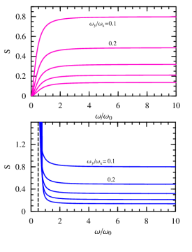
Figure 2: Entanglement entropy $S=S(\rho_{\mu})$ (Eq. (39)) between the two modes as a function of $\omega$ in the vacuum of Hamiltonian (1) at fixed $k_{\mu}=\omega_{\mu}^{2}$, for ratios $\omega_{y}/\omega_{x}=0.1,\ldots,0.5$ and $\omega_{0}=|\omega_{x}|$. The top panel corresponds to sector A (attractive potential $k_{\mu}>0$), the bottom panel to sector B (repulsive potential $k_{\mu}<0$, $|\omega|>\omega_{c}$), where $S$ diverges for $\omega\rightarrow\omega_{c}$ (Eq. (11)). In both cases $S$ approaches the same finite limit for $\omega\rightarrow\infty$.

In contrast, $f_{\mu}$, and hence entanglement, will diverge at the edges of the dynamically stable region. For instance, if $\omega_{y}\rightarrow 0$, $\bar{\omega}\rightarrow\omega_{x}/2$ whereas $\bar{\omega}_{g}\rightarrow 0$, implying $f_{\mu}\propto 1/\sqrt{\omega_{y}}$:

$${f_{\mu}\approx\frac{1}{2}\left[\sqrt{\frac{\bar{\omega}}{2\omega_{y}}}\frac{\omega}{\sqrt{\bar{\omega}^{2}+\omega^{2}}}-1\right]\,,}$$ (55)

and hence $S(\rho_{\mu})\approx\frac{1}{2}\log(\omega_{x}/\omega_{y})$ plus constant terms. This divergence stems from that of $\langle Q_{y}^{2}\rangle$ (or $\langle P_{x}^{2}\rangle$) in this limit, with $\langle P_{y}^{2}\rangle$ and $\langle Q_{x}^{2}\rangle$ remaining constant (Eqs. (31)–(34)).

In the repulsive sector $B$, $f_{\mu}$ diverges for $\omega\rightarrow|\bar{\omega}|=\omega_{c}$ (Eq. (11)), where both $\langle Q_{\mu}^{2}\rangle$ and $\langle P_{\mu}^{2}\rangle$ diverge:

$${f_{\mu}\approx\frac{1}{2}\left[\sqrt{\frac{|\bar{\omega}|}{\omega-|\bar{\omega}|}}\sqrt{\frac{|\bar{\omega}|^{2}-|\bar{\omega}_{g}|^{2}}{2|\bar{\omega}_{g}|^{2}}}-1\right]}\,.$$ (56)

It is then seen that here $f_{\mu}$ and hence $S(\rho_{\mu})$ decrease as $\omega$ increases from $\omega_{c}$ (Fig. 2, bottom panel), i.e., as the system becomes dynamically stabilized by the field, reaching for $\omega\rightarrow\infty$ the same previous limit (54). At fixed $|k_{y}/k_{x}|$, the vacuum entanglement is then strictly larger in the unstable sector $B$ ($k_{\mu}<0$).

At fixed $k^{\prime}_{\mu}$ (rotating potential) the behavior with frequency is quite different (Fig. 3). We should now replace

$$\omega_{\mu}=\sqrt{{\omega^{\prime}_{\mu}}^{2}-\omega^{2}},\;\;\omega^{\prime}_{\mu}=\sqrt{k^{\prime}_{\mu}}\,,$$ (57)

in Eqs. (41)–(42). For $\omega^{\prime}_{x}=\omega^{\prime}_{y}$ there is of course no entanglement. For $|\omega^{\prime}_{x}-\omega^{\prime}_{y}|\ll\omega_{x}$, we have

$${f_{\mu}\approx\frac{\omega^{2}}{16(\omega^{2}-{\omega^{\prime}}_{x}^{2})^{2}}(\omega^{\prime}_{x}-\omega^{\prime}_{y})^{2}+O((\omega^{\prime}_{x}-\omega^{\prime}_{y})^{4})\,.}$$ (58)

Entanglement also vanishes for $\omega\rightarrow 0$, where Eq. (53) still holds ($\omega^{\prime}_{\mu}=\omega_{\mu}$ at $\omega=0$).

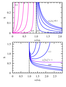
Figure 3: Entanglement entropy between the two modes as a function of $\omega$ in the vacuum of Hamiltonian (1) at fixed $k^{\prime}_{\mu}={\omega^{\prime}_{\mu}}^{2}$, for ratios $\omega^{\prime}_{y}/\omega^{\prime}_{x}=0.1,0.3,\ldots,0.9$ (top) and $(\omega^{\prime}_{y}/\omega^{\prime}_{x})^{2}=-1.3,-1.2,\ldots,-0.7$ (bottom), with $\omega^{\prime}_{0}=\omega^{\prime}_{x}$. The top panel corresponds to $k^{\prime}_{\mu}>0$, with the positive definite sector A on the left, where $S$ diverges for $\omega\rightarrow\omega^{\prime}_{c1}=\omega^{\prime}_{y}$, and the non-positive sector $B_{1}$ on the right ($\omega>\omega^{\prime}_{c2}=\omega^{\prime}_{x}$), where $S$ diverges at $\omega^{\prime}_{x}$ and vanishes for $\omega\rightarrow\infty$. The bottom panel corresponds to $k^{\prime}_{x}>0$ and $k^{\prime}_{y}<0$ (sector $B_{2}$), where $S$ diverges for $\omega\rightarrow\omega^{\prime}_{x}$ and also $\omega\rightarrow\omega^{\prime}_{c3}$ (Eq. (15)) if $(\omega^{\prime}_{y}/\omega^{\prime}_{x})^{2}<-1$. In the critical case $(\omega^{\prime}_{y}/\omega^{\prime}_{x})^{2}=-1$ ($k^{\prime}_{y}=-k^{\prime}_{x}$), $f_{\mu}$ and $S$ saturate for large $\omega$ (Eq. (62)).

On the other hand, as $\omega$ increases, $f_{\mu}$ increases rapidly and in contrast with the previous case, it diverges for $\omega\rightarrow\omega^{\prime}_{c1}$ (Eq. (12)), where, assuming $\omega^{\prime}_{c1}=\omega^{\prime}_{y}<\omega^{\prime}_{x}$,

$${f_{\mu}\approx\frac{1}{2}\left[\sqrt[4]{\frac{{\omega^{\prime}}^{3}_{y}({\omega^{\prime}}^{2}_{x}-{\omega^{\prime}}^{2}_{y})}{2(\omega^{\prime}_{y}-\omega)(3{\omega^{\prime}}_{y}^{2}+{\omega^{\prime}}_{x}^{2})^{2}}}-1\right]\,,}$$ (59)

implying $S(\rho_{\mu})\approx\frac{1}{4}\ln[\omega^{\prime}_{y}/(\omega^{\prime}_{y}-\omega)]$ plus constant terms. In this limit $\langle Q_{y}^{2}\rangle$ and $\langle P_{x}^{2}\rangle$ diverge while $\langle Q_{x}^{2}\rangle$ and $\langle P_{y}^{2}\rangle$ stay constant, as $\omega_{y}=\sqrt{{\omega^{\prime}_{y}}^{2}-\omega^{2}}\rightarrow 0$. As $\omega$ increases further, the system enters the instability window, although for $\omega>{\omega^{\prime}}_{c2}$ (Eq. (13)), it recovers a discrete spectrum, entering sector $B_{1}$. For $\omega\rightarrow{\omega}^{\prime}_{c2}$, $f_{\mu}$ diverges as in (59), with $\omega^{\prime}_{y}\leftrightarrow\omega^{\prime}_{x}$ if ${\omega}^{\prime}_{c2}=\omega^{\prime}_{x}$.

In sector $B_{1}$, $f_{\mu}$ and hence the entanglement decrease as $\omega$ increases, vanishing for $\omega\rightarrow\infty$, in contrast with the behavior at fixed $k_{\mu}$ in sector $A$. In this limit the vacuum of $H$ becomes now that associated with $\omega L_{z}$, which is an isotropic product gaussian state with $L_{z}=0$, and hence zero entanglement. $\langle Q_{\mu}^{2}\rangle$ and $\langle P_{\mu}^{2}\rangle$ stay then finite and their product approaches minimum uncertainty, leading to

$${f_{\mu}\approx\frac{({\omega^{\prime}}_{x}^{2}-{\omega^{\prime}}_{y}^{2})^{2}}{32\,\omega^{2}({\omega^{\prime}}^{2}_{x}+{\omega^{\prime}}_{y}^{2})}+O(\omega^{-4})}\,.$$ (60)

In the unstable domain $B_{2}$, the behavior with $\omega$ is the same as in $B_{1}$ when $k^{\prime}_{x}>0$ and $-k^{\prime}_{x}<k^{\prime}_{y}<0$. However, for $k^{\prime}_{x}>0$ and $-3k^{\prime}_{x}<k^{\prime}_{y}<-k^{\prime}_{x}$, we also have the upper instability limit (15) ($\omega^{\prime}_{c3}$). In this case $f_{\mu}$ first decreases with increasing $\omega$, reaching a minimum, but then starts again to increase, diverging for $\omega\rightarrow\omega^{\prime}_{c3}$ where now both $\langle Q_{\mu}^{2}\rangle$ and $\langle P_{\mu}^{2}\rangle$ diverge, leading to

$${f_{\mu}\approx\frac{1}{2}\left[\sqrt{\frac{\omega^{\prime}_{c3}}{2(\omega^{\prime}_{c3}-\omega)}}-1\right]}\,.$$ (61)

We then obtain different $O(\omega-\omega_{c})^{-1/4}$ and $O(\omega_{c}-\omega)^{-1/2}$ divergences of $f_{\mu}$ at the stability borders $\omega^{\prime}_{x}$ and $\omega^{\prime}_{c3}$ respectively.

In the special critical case $k^{\prime}_{y}=-k^{\prime}_{x}$ $(\omega^{\prime}_{y}=i\omega^{\prime}_{x}$), where $\omega^{\prime}_{c3}\rightarrow\infty$, Eq. (41) leads to

$${f_{\mu}=\frac{1}{2}[\sqrt{1+\frac{\omega^{2}}{\sqrt{\omega^{4}-{\omega^{\prime}}_{x}^{2}}}}-1]}\,,$$ (62)

and hence to a finite asymptotic limit $f_{\mu}=\frac{1}{2}(\sqrt{2}-1)$ for $\omega\rightarrow\infty$, in contrast with (60), as also appreciated in Fig. 3. In this limit $\langle Q_{\mu}^{2}\rangle$ diverges whereas $\langle P_{\mu}^{2}\rangle$ vanishes, the product approaching $1/2$. Hence, as $\omega$ increases, $f_{\mu}$ vanishes if $k^{\prime}_{y}<-k^{\prime}_{x}$, saturates if $k^{\prime}_{y}=-k^{\prime}_{x}$, and diverges (at $\omega=\omega^{\prime}_{c3}$) if $-3k^{\prime}_{x}<k^{\prime}_{y}<-k^{\prime}_{x}$.

The behavior of $f_{\mu}$ (and hence $S(\rho_{\mu})$) with $\omega$ is qualitatively similar to that of the average angular momentum $\langle L_{z}\rangle$. At fixed $k_{\mu}$, the latter also saturates for $\omega\rightarrow\infty$ ($\langle L_{z}\rangle\rightarrow(\bar{\omega}/\bar{\omega}_{g})^{2}-1$) and diverges for $\omega\rightarrow\omega_{c}$ ($\langle L_{z}\rangle\propto(\omega-\omega_{c})^{-1/2}$), whereas at fixed $k^{\prime}_{\mu}$ it diverges for $\omega\rightarrow\omega^{\prime}_{ci}$ ($\langle L_{z}\rangle\propto(\omega-\omega^{\prime}_{ci})^{-1/2}$ for $i=1,2$) and vanishes for $\omega\rightarrow\infty$. Entanglement is then an increasing function of $|\langle L_{z}\rangle|$ at fixed $k_{\mu}$ or $k^{\prime}_{\mu}$, as seen in Fig. 4, although it is not fully determined by $|\langle L_{z}\rangle|$, as the latter is not invariant under local transformations (in contrast with $f_{\mu}$). At fixed $\langle L_{z}\rangle$, higher ratios $k_{y}/k_{x}<1$ originate a higher entanglement (Fig. 4). For small $\omega$, $\langle L_{z}\rangle\propto\omega$ and hence, $f_{\mu}\propto\langle L_{z}\rangle^{2}$ for small $\langle L_{z}\rangle$ in sector $A$. However, at fixed $k^{\prime}_{\mu}$, $\langle L_{z}\rangle$ also vanishes for large $\omega$, where $\langle L_{z}\rangle\propto\omega^{-3}$. Hence, in sector $B_{1}$ and according to Eq. (60), $f_{\mu}\propto\langle L_{z}\rangle^{2/3}$ for small $\langle L_{z}\rangle$, leading to an infinite initial slope (dotted line in Fig. 4). At fixed $\langle L_{z}\rangle$ and $k^{\prime}_{\mu}$, entanglement is then stronger in the unstable sector $B_{1}$ ($\omega>\omega^{\prime}_{c2}$). An exceptional behavior occurs in the critical case $k^{\prime}_{y}=-k^{\prime}_{x}$ (Eq. (62)), where for $\omega\rightarrow\infty$, $\langle L_{z}\rangle\propto\omega^{-2}$ vanishes while $f_{\mu}$ remains finite. In this special limit there is finite entanglement with vanishing angular momentum. On the other hand, close to the divergences, $f_{\mu}\propto\langle L_{z}\rangle$ ($\omega\rightarrow\omega_{c}$) or $\langle L_{z}\rangle^{1/2}$ ($\omega\rightarrow\omega^{\prime}_{ci}$, $i=1,2$), implying $S(\rho_{\mu})\propto\ln\,\langle L_{z}\rangle$ for large $\langle L_{z}\rangle$.

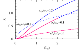
Figure 4: The entanglement entropy between the two modes as a function of the scaled average angular momentum $\langle L_{z}\rangle=\langle{\cal L}_{z}\rangle/\hbar$ (Eq. (5)), in the vacuum of (1) at fixed $k_{\mu}=\omega_{\mu}^{2}$ (solid and dashed lines) and at fixed $k^{\prime}_{\mu}={\omega^{\prime}_{\mu}}^{2}$ (dashed-dotted and dotted lines), for selected ratios $\omega_{y}/\omega_{x}$ and $\omega^{\prime}_{y}/\omega^{\prime}_{x}$ and variable $\omega$. The solid and dashed-dotted lines (in red) correspond to sector A ($k_{\mu}>0$ or $k^{\prime}_{\mu}>0$ and $|\omega|<\omega^{\prime}_{y}$), the dashed and dotted lines (in blue) to sector B ($k_{\mu}<0$, $|\omega|>\omega_{c}$) and $B_{1}$ ($k^{\prime}_{\mu}>0$, $|\omega|>\omega^{\prime}_{x}$). $S$ is in all sectors an increasing function of $|\langle L_{z}\rangle|$.

III.2 Thermal entanglement

Let us now examine the thermal entanglement in the stable sector $A$. We first depict in Fig. 5 the limit temperature for entanglement $T_{E}$, determined from the condition $\tilde{f}_{-}=0$ (equality in Eq. (48)). This temperature remains finite for all values of $k_{\mu}$ or $k^{\prime}_{\mu}$, including the edge of the sector ($k_{\mu}\rightarrow 0$ or $|\omega|\rightarrow\sqrt{k^{\prime}_{\mu}}$), where the vacuum $f_{\mu}$ diverges. At the edge, $\lambda_{-}\rightarrow 0$ and hence a finite $T$ already gives rise to a spread over all energy levels ($f^{\prime}_{-}\rightarrow\infty$), which diminishes and eventually kills the entanglement. A related fundamental effect is that at finite $T>0$, entanglement does not diverge at the edge, but stays finite or vanishes, depending on the value of $T$.

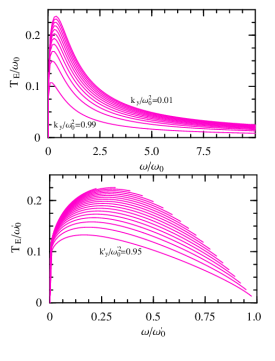
Figure 5: Top: Scaled limit temperatures for entanglement $T_{E}$ at fixed $k_{\mu}$ (top) and at fixed $k^{\prime}_{\mu}$ (bottom), as a function of frequency for different ratios $k_{y}/k_{x}=0.01,0.1,\ldots,0.9,0.99$ (top) and $k^{\prime}_{y}/k^{\prime}_{x}=0.05,0.1,\ldots,0.95$ (bottom), with $\omega_{0}=\omega_{x}=\sqrt{k_{x}}$, $\omega^{\prime}_{0}=\omega^{\prime}_{x}=\sqrt{k^{\prime}_{x}}$. At fixed $k_{\mu}$, $T_{E}$ vanishes for large $\omega$ (Eq. (65)) whereas at fixed $k^{\prime}_{\mu}$, it approaches a finite value at the upper stability limit $\omega^{\prime}_{c1}=\sqrt{k^{\prime}_{y}}$.

More precisely, for $\omega_{y}\rightarrow 0$ and fixed $\omega_{x}>0$, $\lambda_{+}\rightarrow\sqrt{4\omega^{2}+\omega_{x}^{2}}$ whereas $\lambda_{-}\approx\omega_{y}\omega_{x}/\lambda_{+}$, implying $f^{\prime}_{-}\approx T/\lambda_{-}\approx T\lambda_{+}/(\omega_{x}\omega_{y})$. Hence, in this limit Eqs. (44)–(46) lead to

$$\tilde{f}_{-}=\frac{1}{2}[\sqrt{\frac{T\lambda_{+}^{4}(1+2f^{\prime}_{+})^{2}}{\omega_{x}^{2}(2\omega^{2}\lambda_{+}(1+2f^{\prime}_{+})+T\omega_{x}^{2})}}-1]\,,$$ (63)

which remains finite and above $-1/2$ if $T>0$. This implies a finite negativity in this limit if $T>0$, with $N\propto T^{-1/2}$ for $T\rightarrow 0$ according to Eq. (47). Therefore, at finite temperature the vacuum divergences of the entanglement can be only probed indirectly, through the $T^{-1/2}$ behavior of $N$ near the edge at sufficiently low $T$.

In addition, Eq. (63) entails a finite limit temperature $T_{E}$, obtained from the condition $\tilde{f}_{-}=0$ in (63):

$$T_{E}={\frac{2(1+2f^{\prime}_{+})\omega^{2}\omega_{x}^{2}\lambda_{+}}{(1+2f^{\prime}_{+})^{2}\lambda_{+}^{4}-\omega_{x}^{4}}}\,,$$ (64)

which is a transcendental equation for $T_{E}$ ($f^{\prime}_{+}$ depends on $T_{E}$). The maximum limit temperature $T_{E}^{M}$ at fixed $k_{x}=\omega_{x}^{2}$ or ${T^{\prime}}_{E}^{M}$ at fixed $k^{\prime}_{x}={\omega^{\prime}_{x}}^{2}$, is in fact obtained in this limit ($\omega_{y}=0$ or $\omega^{\prime}_{y}=\omega$): At fixed $k_{x}$, $T_{E}^{M}\approx 0.24\omega_{x}$, attained at $\omega\approx 0.38\omega_{x}$, while at fixed $k^{\prime}_{x}$, ${T^{\prime}}_{E}^{M}\approx 0.23{\omega^{\prime}_{x}}$, attained at $\omega\approx 0.28{\omega^{\prime}}_{x}$.

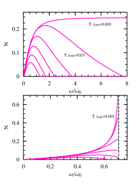
Figure 6: Top: Negativity as a function of frequency at increasing temperatures $T/\omega_{0}=0.001,0.03,0.06,\ldots,0.15$, at fixed $k_{\mu}$ (top), for $k_{y}/k_{x}=0.2$, and at fixed $k^{\prime}_{\mu}$ (bottom), for $k^{\prime}_{y}/k^{\prime}_{x}=0.5$. At $T>0$, $N$ is finite, and non-zero just within a finite frequency window.

At fixed $k_{\mu}$, the limit temperature $T_{E}$ as a function of $\omega$ exhibits first a maximum and then vanishes for $\omega\rightarrow\infty$ (top panel in Fig. 5), i.e., in the limit where the vacuum entanglement saturates. The reason is that $\lambda_{-}$ also vanishes for $\omega\rightarrow\infty$ ($\lambda_{-}\approx\omega_{x}\omega_{y}/(2\omega)$), implying $T_{E}\propto\omega^{-1}$ in this limit:

$$T_{E}\approx\frac{\omega_{x}\omega_{y}}{2\omega\ln\frac{\omega_{x}+\omega_{y}}{\omega_{x}-\omega_{y}}}\,.$$ (65)

In fact, for $\omega\rightarrow\infty$ and fixed $k_{\mu}$ (with $k_{y}<k_{x}$), Eqs. (44)–(46) lead to

$$\tilde{f}_{-}\approx\frac{1}{2}[\sqrt{\frac{(1+2f^{\prime}_{-})\omega_{y}}{\omega_{x}}}-1]\,,$$ (66)

such that $\tilde{f}_{-}=0$ for $1+2f^{\prime}_{-}=\omega_{x}/\omega_{y}$, which leads to Eq. (65). On the other hand, for $\omega\rightarrow 0$, $T$ vanishes logarithmically ($T_{E}\propto-1/\ln\omega$) and the same occurs for $\omega_{y}\rightarrow\omega_{x}$, since in these limits $\lambda_{\pm}$ remain both finite whereas the negativity vanish. At fixed $T$, we then obtain a finite frequency window for entanglement, which narrows for increasing temperature or decreasing anisotropy, as seen in Fig. 5 and also Fig. 6, where the negativity (47) is depicted. Let us remark that entanglement ceases to be correlated with $\langle L_{z}\rangle$ as the temperature increases ($\langle L_{z}\rangle\propto\omega T$ for high $T$).

At fixed $k^{\prime}_{\mu}$, the behavior of $T_{E}$ and $N$ look quite different, as now $\omega$ is bounded above by $\omega^{\prime}_{y}$ (assuming $\omega^{\prime}_{y}<\omega^{\prime}_{x}$). For $\omega\rightarrow\omega^{\prime}_{y}$, $T_{E}$ is then determined by Eq. (64) with $\omega_{x}\rightarrow\sqrt{{\omega^{\prime}_{x}}^{2}-\omega^{2}}$, and remains finite. Actually, as verified in the bottom panel of Fig. 5, $T_{E}$ acquires in this border its maximum value as $\omega$ increases at fixed $k^{\prime}_{\mu}$ if $\omega^{\prime}_{y}<\omega^{\prime}_{yc}\approx 0.28\omega^{\prime}_{x}$, while if $\omega^{\prime}_{y}>\omega^{\prime}_{yc}$ the maximum is attained at an intermediate frequency. Consequently, at fixed $T<{T^{\prime}}_{E}^{M}$ there is again entanglement within a certain frequency window, which extends up to the stability border $\omega=\omega^{\prime}_{y}$ if $\omega^{\prime}_{y}<\omega^{\prime}_{yc}$ or $T<T_{E}$ at $\omega=\omega^{\prime}_{y}$ (bottom panel in Fig. 6). The absolute maximum ${T^{\prime}}_{E}^{M}$ is obtained at this border precisely at $\omega^{\prime}_{y}=\omega^{\prime}_{yc}$. For $\omega\rightarrow 0$ or $\omega^{\prime}_{y}\rightarrow\omega^{\prime}_{x}$, $T_{E}$ decreases again logarithmically.

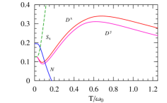
Figure 7: Negativity ($N$), single mode entropy $S_{x}=S(\rho_{x})$ and the quantum discords $D^{y}$ and $D^{x}$ as a function of temperature for $\omega=\omega_{0}=\sqrt{k_{x}}$ and $k_{y}=0.2k_{x}$.

III.3 Comparison with the quantum discord

We finally compare in Fig. 7 the thermal behavior of the negativity with that of the gaussian quantum discord $D^{y}$ (Eq. (51)) and also $D^{x}$. For reference we have also plotted the entropy of one of the modes ($x$), no longer a measure of entanglement, just to indicate its coincidence with both $D^{y}$ and $D^{x}$ for $T\rightarrow 0$. While at $T=0$ the negativity is just an increasing function of the entanglement entropy (Eqs. (49)–(39)) and hence of the quantum discord, the behavior for $T>0$ is quite different. Although exhibiting a similar initial decreasing trend (essentially due to the initial increase of the total entropy $S(\rho_{AB})$ in (50)) the gaussian discord starts then to increase (due to the increase in the first term of (50)), vanishing only asymptotically for $T\rightarrow\infty$. Such revival of the discord with increasing $T$ was also observed in spin systems WR.10 ; MG.10 , and reflects the presence of quantum correlations in the excited eigenstates, which lead at these temperatures to a separable yet not classically correlated (in the sense of sec. II.6) thermal state. Since $D^{\mu}>1$ implies entanglement GP.10 ; AD.10 , one can ensure here that $D^{\mu}<1$ after the vanishing of the negativity ($T>T_{E}$), although this may not prevent $D^{\mu}$ from reaching a higher value than at $T=0$ at some intermediate temperature, as seen in Fig. 7. For $T\rightarrow\infty$ we actually obtain, from Eq. (51) and the expression of AD.10 , that $D^{\mu}\propto T^{-1}$:

$$D^{y}\approx\frac{\omega^{2}}{2T\sqrt{\omega^{2}+\omega_{x}^{2}}}\,,$$ (67)

with a similar expression for $D^{x}$ after replacing $\omega_{x}$ by $\omega_{y}$. Hence, for high $T$ $D^{\mu}$ becomes independent of $\omega_{\mu}$, with $D^{x}>D^{y}$ asymptotically if $\omega_{y}<\omega_{x}$, as verified in Fig. 7. We also remark that the discord remains finite for $T>0$ in the whole sector $A$.

IV Conclusions

We have analyzed the entanglement induced by an angular momentum coupling on two harmonic modes. Full analytic expressions for the vacuum entanglement entropy and the thermal negativity were derived. The model exhibits a rich phase structure and admits distinct physical realizations (particle in a magnetic field in an anisotropic harmonic trap, or particle in a rotating harmonic trap), which lead to different entanglement behaviors with the relevant control parameter. For instance, in sector A (stable vacuum), entanglement saturates for strong fields in the first case, but diverges at a finite frequency in the second case. Vacuum entanglement diverges at the onset of instabilities, being correlated with the average angular momentum and reaching higher values in unstable domains dynamically stabilized by the field or rotation. In contrast, thermal entanglement is finite, and non-zero just below a finite limit temperature within a reduced frequency window, diverging only for $T\rightarrow 0$ at the instability borders. We have also shown that after a short initial common trend, the thermal behavior of the gaussian quantum discord becomes substantially different from that of entanglement, vanishing only asymptotically. A deeper investigation of the discord and other related measures of quantum correlations AD.11 ; RCC.10 in similar systems is being undertaken.

The authors acknowledge support from CONICET (LR) and CIC (RR) of Argentina.

References

- (1) M.A. Nielsen and I.L. Chuang, Quantum Computation and Quantum Information (Cambridge Univ. Press, Cambridge, UK, 2000).
- (2) V. Vedral, Introduction to Quantum Information Science (Oxford Univ. Press, Oxford, UK 2006).
- (3) L. Amico, R. Fazio, A. Osterloh and V. Vedral, Rev. Mod. Phys. 80, 516 (2008).
- (4) R. Horodecki, P. Horodecki, M. Horodecki and K. Horodecki, Rev. Mod. Phys. 81, 865 (2009).
- (5) R. Simon, Phys. Rev. Lett. 84, 2726 (2000).
- (6) L.M. Duan, G. Giedke, J.I. Cirac, P. Zoller, Phys. Rev. Lett. 84, 2722 (2000).
- (7) R.F. Werner, M.M. Wolf, Phys. Rev. Lett. 86, 3658 (2001).
- (8) K. Audenaert, J. Eisert, M.B. Plenio, and R.F. Werner, Phys. Rev. A 66, 042327 (2002).
- (9) G. Adesso, A. Serafini, and F. Illuminati, Phys. Rev. A 70, 022318 (2004); A. Serafini, G. Adesso, and F. Illuminati, Phys. Rev. A 71, 032349 (2005).
- (10) M. Cramer, J. Eisert, M.B. Plenio, and J. Dreißig, Phys. Rev. A 73, 012309 (2006).
- (11) G. Adesso, F. Illuminati, Phys. Rev. A 78, 042310 (2008).
- (12) J.M. Matera, R. Rossignoli, N. Canosa, Phys. Rev. A 82, 052332 (2010).
- (13) C.H. Bennett, H.J. Bernstein, S. Popescu, and B. Schumacher, Phys. Rev. A 53, 2046 (1996).
- (14) K. Zyczkowski, P. Horodecki, A. Sanpera, and M. Lewenstein, Phys. Rev. A 58, 883 (1998).
- (15) G. Vidal, R.F. Werner, Phys. Rev. A 65, 032314 (2002).
- (16) A. Peres, Phys. Rev. Lett. 77, 1413 (1996).
- (17) M. Horodecki, P. Horodecki and R. Horodecki, Phys. Lett. A 223, 1 (1996).
- (18) S.L. Braunstein and P. van Loock, Rev. Mod. Phys. 77, 513 (2005).
- (19) H. Ollivier and W.H. Zurek, Phys. Rev. Lett. 88, 017901 (2001).
- (20) L. Henderson and V. Vedral, J. Phys. A 34, 6899 (2001).
- (21) P. Giorda, M.G.A. Paris, Phys. Rev. Lett. 105, 020503 (2010).
- (22) G. Adesso, A. Datta, Phys. Rev. Lett. 105, 030501 (2010).
- (23) A. Datta, A. Shaji, and C.M. Caves, Phys. Rev. Lett. 100, 050502 (2008).
- (24) E. Knill, R. Laflamme, Phys. Rev. Lett. 81, 5672 (1998).
- (25) A. Datta, S.T. Flammia and C.M. Caves, Phys. Rev. A 72, 042316 (2005).
- (26) D. Cavalcanti et al, Phys. Rev. A 83, 032324 (2011).
- (27) A. Streltsov, H. Kampermann, and D. Bruß, Phys. Rev. Lett. 106, 160401 (2011).
- (28) M. Piani et al, Phys. Rev. Lett. 106, 220403 (2011).
- (29) J.G. Valatin, Proc. R. Soc. London 238, 132 (1956).
- (30) A. Feldman and A. H. Kahn, Phys. Rev. B 1, 4584 (1970).
- (31) P. Ring and P. Schuck, The Nuclear Many-Body Problem, (Springer, NY, 1980).
- (32) J.P. Blaizot and G. Ripka, Quantum Theory of Finite Systems (MIT Press, MA, 1986).
- (33) A.V. Madhav, T. Chakraborty, Phys. Rev. B 49, 8163 (1994).
- (34) M. Linn, M. Niemeyer, and A. L. Fetter, Phys. Rev. A 64, 023602 (2001).
- (35) M. Ö. Oktel, Phys. Rev. A 69, 023618 (2004).
- (36) A. L. Fetter, Phys. Rev. A 75, 013620 (2007).
- (37) A. Aftalion, X. Blanc, and N. Lerner, Phys. Rev. A 79, 011603(R) (2009).
- (38) A. Aftalion, X. Blanc, J. Dalibard, Phys. Rev. A 71, 023611 (2005); S. Stock et al, Laser Phys. Lett. 2, 275 (2005).
- (39) I. Bloch, J. Dalibard, W. Zwerger, Rev. Mod. Phys. 80, 885 (2008).
- (40) A.Ł. Fetter, Rev. Mod. Phys. 81, 647 (2009).
- (41) J. Pěrina, Z. Hradil, and B. Jurčo, Quantum optics and Fundamentals of Physics (Kluwer, Dordrecht, 1994); N. Korolkova, J. Pěrina, Opt. Comm. 136, 135 (1996).
- (42) R. Rossignoli and A.M. Kowalski, Phys. Rev. A 79 062103 (2009).
- (43) A.P. Hines, R. H. McKenzie, and G.J. Milburn, Phys. Rev. A 67, 013609 (2003).
- (44) H.T. Ng, P.T. Leung, Phys. Rev. A 71, 013601 (2005).
- (45) A.V. Chizhov, R.G. Nazmitdinov, Phys. Rev. A 78, 064302 (2008).
- (46) R.F. Werner, Phys. Rev. A 40, 4277 (1989).
- (47) A. Ferraro et al, Phys. Rev. A 81, 052318 (2010).
- (48) L. Mišta et al, Phys. Rev. A 83, 042325 (2011).
- (49) T. Werlang and G. Rigolin, Phys. Rev. A 81, 044101 (2010).
- (50) J. Maziero et al, Phys. Rev. A 82, 012106 (2010).
- (51) R. Rossignoli, N. Canosa and L. Ciliberti, Phys. Rev. A 82, 052342 (2010).