We investigate the production of positive parity baryon resonances in proton electromagnetic scattering within the Sakai-Sugimoto model. The latter is a string model for the non-perturbative regime of large $N_{c}$ QCD. Using holographic techniques we calculate the generalized Dirac and Pauli form factors that describe resonance production. We use these results to estimate the contribution of resonance production to the proton structure functions. Interestingly, we find an approximate Callan-Gross relation for the structure functions in a regime of intermediate values of the Bjorken variable.

Generalized baryon form factors and proton structure functions in the Sakai-Sugimoto model

1 Introduction

In the regime of low momentum transfer ($\sqrt{q^{2}}$ lower than a few $GeVs$), non-perturbative effects become relevant in hadronic scattering. Lattice QCD (the numerical approach of substituting the continuous spacetime by a lattice of points) is quite difficult to use here because of the real time dependence in scattering processes. Effective models can be very useful but they have a low predictability because they may depend on many parameters.

In recent years, gauge/string duality has evolved into an invaluable tool to study many strongly coupled phenomena in particle and condensed matter physics. In particular, it has brought a new insight into the strongly coupled regime of Yang-Mills theories. A good example is the successful prediction of the shear viscosity for strongly coupled theories whose gravity dual involves a black hole in Anti-de-Sitter space [1]. This prediction is in accordance with the small value observed in the quark-gluon plasma phase observed in heavy ion collisions at RHIC and LHC. The study of 10-d string models (top-down approach) and 5-d effective models (bottom-up approach) dual to 4-d QCD-like theories is known as AdS/QCD (see [2, 3, 4, 5] for a review of the top-down approach, [6, 7, 8] for the bottom-up approach and [9] for an hybrid approach). AdS/QCD is a powerful approach to the strong coupling regime of QCD because the string models depend on very few parameters (the string length, string coupling and number of colors and flavours of the dual theory). On top of that, general properties of hadron phenomenology (like vector meson dominance) seem to be universal in this approach in the sense that they do not depend on the particular AdS/QCD model. There is one string model, though, that has a field content very similar to large $N_{c}$ QCD in the regime of large distances and massless quarks. This is the Sakai-Sugimoto model [10, 11] that realizes confinement and chiral symmetry breaking.

In this paper we investigate the production of baryon resonances with positive parity in proton electromagnetic scattering within the Sakai-Sugimoto model. First we define the current matrix element that describe the transition from a proton to a positive parity baryonic resonance. We derive the general expansion of the current matrix element in terms of scalars that we define as generalized Dirac and Pauli form factors which include as a particular case the well known elastic Dirac and Pauli form factors. Using holographic techniques we obtain a relation between the generalized Dirac and Pauli form factors and the couplings between baryons and vector mesons. This result can be interpreted as a realization of vector meson dominance in electromagnetic scattering of baryons.

We also estimate in this paper the contribution of resonance production to the proton structure functions. The latter are Lorentz invariant scalars defined in Deep Inelastic Scatering (DIS) which is the inclusive scattering of a proton by a virtual photon (emitted by a lepton). The proton structure functions have a nice interpretation in terms of parton distribution functions that describe probability densities of finding partons (valence quarks, gluons and quark-antiquark pairs) with a fraction of the longitudinal momentum of the proton. A calculation of these quantities at low momentum transfer proves difficult in non-perturbative QCD and usually relies heavily on some input from experiments or simulations. It should be noted that in the Sakai-Sugimoto model we can only make reliable predictions about scattering processes with low momentum transfers ( in this paper $q^{2}\leq 5({\text{G}eV})^{2}$). This regime is very far from the Bjorken limit of DIS ($q^{2}\to\infty$) which is well described by perturbative QCD. Moreover, it is beyond the scope of this paper to study the full inclusive DIS process with arbitrary final states. Therefore we limit ourselves to the contribution coming from single final state baryons with the same spin and isospin as the proton but different masses.

Electromagnetic form factors have been obtained previously using bottom-up (phenomenological) models and top-down string models. The meson form factors have been calculated in [14, 15, 16] (bottom-up) and [17, 18, 19, 20] (top-down). Baryon form factors have been obtained in [21, 22] (bottom-up) and [23, 24, 25, 26] (top-down). Deep Inelastic Scattering in AdS/QCD was first investigated by Polchinski and Strassler in a bottom-up model for the case of scalar glueballs and baryon-like fermions [27]. Further development of DIS in bottom-up and top-down models include the large $x$ regime [28, 29, 30, 31] as well as the small $x$ regime where Pomeron exchange dominates [32, 33, 34, 35, 36, 37]. DIS structure functions have also been calculated for strongly coupled plasmas [38, 39, 40, 41].

The discussion in section 2 is independent of a specific model realization and contains novel results that apply very generally to non-elastic electromagnetic scattering for baryons, namely a detailed derivation of electromagnetic current matrix elements and structure functions. In section 3 we briefly review the Sakai-Sugimoto model and the description of holographic baryons in this context. Section 4 contains the derivation of the electromagnetic current and the generalized Dirac and Pauli form factors. Numerical results for the wave functions, masses, couplings and form factors are presented for the lowest excited states of spin $1/2$ and positive parity. In section 5 we present our numerical estimate on the proton structure functions and the associated Callan-Gross relation.

2 Baryon resonances in proton electromagnetic scattering

Massless QCD with $N_{f}$ flavours enjoys chiral symmetry ($U(N_{f})_{L}\times U(N_{f})_{R}$) at high energies. At low energies chiral symmetry is spontaneously broken and the residual symmetry is vectorial corresponding to the group $U(N_{f})_{V}$. In the case of two flavours, the vectorial current can be written as $J_{V}^{\mu,a}$ where $a=(0,1,2,3)$. The electromagnetic current ${\cal J}^{\mu}$ can be obtained as a combination of the isoscalar current $J_{V}^{\mu,0}$ and the isovector current $J_{V}^{\mu,3}$ :

$${\cal J}^{\mu}=\frac{1}{N_{c}}J_{V}^{\mu,0}+J_{V}^{\mu,3}\equiv\sum_{a=0}^{3}c_{a}J_{V}^{\mu,a}\,.$$ (2.1)

In this paper we are interested in the production of baryon resonances with positive parity in electromagnetic scattering of a proton. Namely, we study the transition of a proton (denoted by $B$) with spin $1/2$, isospin $1/2$ and momentum $p$ to a baryonic resonance (denoted by $B_{X}$) with the same spin and isospin as the proton but momentum $p_{X}$ and different mass. This transition is characterized by evaluating the matrix elements of electromagnetic currents between the baryonic initial and final states. We denote the spin and isospin projections of the initial (final) baryon state as $s$ ($s_{X}$) and $I_{3}$ ($I_{3}^{X}$) respectively.

2.1 The generalized Dirac and Pauli form factors

Evaluating the isoscalar and isovector current operators in the baryonic states we obtain current matrix elements that can be decomposed as

$$\langle p_{X},B_{X},s_{X},I_{3}^{X}|J_{V}^{\mu,a}(0)|p,B,s,I_{3}\rangle = \frac{i}{2(2\pi)^{3}}(\tau^{a})_{I_{3}^{X}I_{3}}\bar{u}(p_{X},s_{X})\Big{[}\gamma^{\mu}F^{D,a}_{BB_{X}}(q^{2})$$ (2.2)

$$+ \kappa_{B}\sigma^{\mu\nu}q_{\nu}F^{P,a}_{BB_{X}}(q^{2})\,+\,iq^{\mu}F^{Q,a}_{BB_{X}}(q^{2})\Big{]}u(p,s)\,,$$ (2.3)

where

$$q^{\mu} = (p_{X}-p)^{\mu}\quad,\quad\kappa_{B}=\frac{1}{m_{B}+m_{B_{X}}}\,,$$ (2.4)

$$(\tau^{0})_{I_{3}^{X}I_{3}} = \delta_{I_{3}^{X}I_{3}}\quad,\quad(\tau^{a})_{I_{3}^{X}I_{3}}=(\sigma^{a})_{I_{3}^{X}I_{3}}\quad a=(1,2,3)\,,$$ (2.5)

and $\sigma^{a}$ are the Pauli matrices. In (2.3) we have used a generalization of the Gordon decomposition identity

$${\bar{u}}_{B_{X}}(p^{\prime})\gamma^{\mu}u_{B}(p)={\bar{u}}_{B_{X}}(p^{\prime})\left[-\frac{p^{\prime\mu}+p^{\mu}}{m_{B}+m_{B_{X}}}+\frac{i\sigma^{\mu\nu}\left(p^{\prime}_{\nu}-p_{\nu}\right)}{m_{B}+m_{B_{X}}}\right]u_{B}(p)\,.$$ (2.6)

The scalars $F^{D,a}_{BB_{X}}(q^{2})$,$F^{P,a}_{BB_{X}}(q^{2})$ in (2.3) are the Dirac and Pauli form factors while $F^{Q,a}_{BB_{X}}(q^{2})$ is required by current conservation

$$0 = q_{\mu}\langle J_{V}^{\mu,a}(0)\rangle\sim\bar{u}(p_{X},s_{X})\Big{[}(p_{X}-p)_{\mu}\gamma^{\mu}F^{D,a}_{BB_{X}}(q^{2})\,+\,iq^{2}F^{Q,a}_{BB_{X}}(q^{2})\Big{]}u(p,s)$$ (2.7)

$$= \bar{u}(p_{X},s_{X})\Big{[}i(m_{B_{X}}-m_{B})F^{D,a}_{BB_{X}}(q^{2})\,+\,iq^{2}F^{Q,a}_{BB_{X}}(q^{2})\Big{]}u(p,s)\,,$$ (2.8)

so that

$$F^{Q,a}_{BB_{X}}(q^{2})=-\frac{1}{q^{2}}(m_{B_{X}}-m_{B})F^{D,a}_{BB_{X}}(q^{2})\,.$$ (2.9)

The current matrix element now takes a transverse form

$$\langle p_{X},B_{X},s_{X}|J_{V}^{\mu,a}(0)|p,B,s\rangle = \frac{i}{2(2\pi)^{3}}(\tau^{a})_{I_{3}^{X}I_{3}}\left(\eta^{\mu\nu}-\frac{q^{\mu}q^{\nu}}{q^{2}}\right)\bar{u}(p_{X},s_{X})\Big{[}\gamma_{\nu}F^{D,a}_{BB_{X}}(q^{2})$$ (2.10)

$$+ \kappa_{B}\sigma_{\nu\lambda}q^{\lambda}F^{P,a}_{BB_{X}}(q^{2})\Big{]}u(p,s)\,.$$ (2.11)

We have chosen the signature $\eta_{\mu\nu}={\rm diag}(-,+,+,+)$. The relativistic Dirac spinors that represent the initial and final states can be written as

$$u(p,s)=\frac{1}{\sqrt{2E}}\left(\begin{array}[]{c}f\,\chi_{s}(\vec{p})\\ \frac{\vec{p}\cdot\vec{\sigma}}{f}\,\chi_{s}(\vec{p})\end{array}\right)\quad,\quad u(p_{X},s_{X})=\frac{1}{\sqrt{2E_{X}}}\left(\begin{array}[]{c}f_{X}\,\chi_{s_{X}}(\vec{p}_{X})\\ \frac{\vec{p}_{X}\cdot\vec{\sigma}}{f_{X}}\,\chi_{s_{X}}(\vec{p}_{X})\end{array}\right)\,,$$ (2.16)

where $f=\sqrt{E+m_{B}}$ and $f_{X}=\sqrt{E_{X}+m_{B_{X}}}$. The two-component spinors $\chi_{s}(\vec{p})$ and $\chi_{s_{X}}(\vec{p}_{X})$ are defined as eigenstates of the helicity operators

$$\frac{\vec{p}\cdot\vec{\sigma}}{|\vec{p}|}\chi_{s}(\vec{p})=s\,\chi_{s}(\vec{p})\quad,\quad\frac{\vec{p}_{X}\cdot\vec{\sigma}}{|\vec{p}_{X}|}\chi_{s_{X}}(\vec{p}_{X})=s_{X}\,\chi_{s_{X}}(\vec{p}_{X})\,.$$ (2.17)

The convention for gamma matrices is

$$\gamma^{0}=-i\left(\begin{array}[]{cc}1&0\\ 0&-1\end{array}\right)\quad,\quad\gamma^{i}=-i\left(\begin{array}[]{cc}0&\sigma^{i}\\ -\sigma^{i}&0\end{array}\right)\quad,\quad\sigma^{\mu\nu}=\frac{i}{2}\left[\gamma^{\mu},\gamma^{\nu}\right]\,.$$ (2.22)

The baryon states are normalized according to their charges as

$$\langle p_{X},B_{X},s_{X},I_{3}^{X}|Q_{V}^{a}|p,B,s,I_{3}\rangle = \langle p_{X},B_{X},s_{X},I_{3}^{X}|J_{V}^{0,a}(0)|p,B,s,I_{3}\rangle(2\pi)^{3}\delta^{3}(\vec{q})$$ (2.23)

$$= \frac{1}{2}(\tau^{a})_{I_{3}^{X}I_{3}}\delta^{3}(\vec{q})\delta_{s_{X}s}\delta_{BB_{X}}F^{D,a}_{BB}(0)\,.$$ (2.24)

In the case where the initial state is a proton and the final state has the same isospin polarization ($I_{3}^{X}=I_{3}=1/2$) the isoscalar and isovector charges are $N_{c}/2$ and $1/2$ respectively. The elastic Dirac form factors are fixed at $q^{2}=0$ as

$$F^{D,0}_{BB}(0)=N_{c}\quad,\quad F^{D,3}_{BB}(0)=1\,,$$ (2.25)

so we find from (2.24)

$$\langle p_{X},B_{X},s_{X},1/2|p,B,s,1/2\rangle = \delta^{3}(\vec{p}_{X}-\vec{p})\delta_{s_{X}s}\delta_{B_{X}B}\,.$$ (2.26)

The following spinor relations are very useful

$$\bar{u}(p_{X},s_{X})\gamma^{0}u(p,s) = -\frac{i}{2\sqrt{EE_{X}}}\chi_{s_{X}}^{\dagger}(\vec{p}_{X})\Big{[}ff_{X}\,+\,\frac{1}{ff_{X}}\vec{p}_{X}\cdot\vec{\sigma}\vec{p}\cdot\vec{\sigma}\Big{]}\chi_{s}(\vec{p})$$ (2.27)

$$= -\frac{i}{2\sqrt{EE_{X}}}\left(\frac{f}{f_{X}}\right)\left[f_{X}^{2}+\frac{s_{X}s|\vec{p}_{X}||\vec{p}|}{f^{2}}\right]\chi_{s_{X}}^{\dagger}(\vec{p}_{X})\chi_{s}(\vec{p})\,,$$ (2.28)

$$\bar{u}(p_{X},s_{X})\gamma^{i}u(p,s) = -\frac{i}{2\sqrt{EE_{X}}}\chi_{s_{X}}^{\dagger}(\vec{p}_{X})\Big{\{}\frac{f_{X}}{f}\sigma^{i}\vec{p}\cdot\vec{\sigma}\,+\,\frac{f}{f_{X}}\vec{p}_{X}\cdot\vec{\sigma}\sigma^{i}\Big{\}}\chi_{s}(\vec{p})$$ (2.30)

$$= -\frac{i}{2\sqrt{EE_{X}}}\left(\frac{f}{f_{X}}\right)\left[\frac{f_{X}^{2}}{f^{2}}s|\vec{p}|+s_{X}|\vec{p}_{X}|\right]\,\chi_{s_{X}}^{\dagger}(\vec{p}_{X})\sigma^{i}\chi_{s}(\vec{p})\,,$$ (2.31)

$$\bar{u}(p_{X},s_{X})\sigma^{0i}q_{i}u(p,s) = -\frac{i}{2\sqrt{EE_{X}}}\left[\frac{f_{X}}{f}q^{i}p^{j}-\frac{f}{f_{X}}(p+q)^{i}q^{j}\right]\,\chi_{s_{X}}^{\dagger}(\vec{p}_{X})\sigma_{i}\sigma_{j}\chi_{s}(\vec{p})$$ (2.33)

$$= -\frac{i}{2\sqrt{EE_{X}}}\left(\frac{f}{f_{X}}\right)\left[\frac{f_{X}^{2}}{f^{2}}s|\vec{p}|-s_{X}|\vec{p}_{X}|\right]\,q_{i}\,\chi_{s_{X}}^{\dagger}(\vec{p}_{X})\sigma^{i}\chi_{s}(\vec{p})\,,$$ (2.34)

$$\bar{u}(p_{X},s_{X})\sigma^{ij}q_{j}u(p,s) = -\frac{1}{2\sqrt{EE_{X}}}\epsilon^{ijk}q_{j}\chi_{s_{X}}^{\dagger}(\vec{p}_{X})\Big{[}f_{X}f\sigma_{k}\,-\,\frac{1}{f_{X}f}(p+q)^{a}p^{b}\sigma_{a}\sigma_{k}\sigma_{b}\Big{]}\chi_{s}(\vec{p})$$ (2.36)

$$= -\frac{1}{2\sqrt{EE_{X}}}\left(\frac{f}{f_{X}}\right)\epsilon^{ijk}q_{j}\left[f_{X}^{2}-\frac{s_{X}s|\vec{p}_{X}||\vec{p}|}{f^{2}}\right]\chi_{s_{X}}^{\dagger}(\vec{p}_{X})\sigma_{k}\chi_{s}(\vec{p})\,.$$ (2.37)

The Breit frame. The Breit frame is characterized by the condition $E_{X}=E$ which means that the photon has zero energy ($q_{0}=0$). As shown in the appendix, choosing the photon in the z axis, the the photon and baryon momenta in the Breit frame take the form

$$q^{\mu} = (0,0,0,q)\quad,\quad p^{\mu}=(E,0,0,p_{3})\quad,\quad p^{\mu}_{X}=p^{\mu}+q^{\mu}\,,$$ (2.39)

$$p_{3} = -\frac{q}{2x}\quad,\quad E=\sqrt{m_{B}^{2}+p_{3}^{2}}\,.$$ (2.40)

Using eq. (2.11) and the spinor relations (LABEL:spinrel1) - (LABEL:spinrel4) we can work out the components of the current matrix elements. In the Breit frame the current matrix elements simplify to

$$\langle p_{X},B_{X},s_{X},I_{3}^{X}|J_{V}^{0,a}(0)|p,B,s,I_{3}\rangle = \frac{1}{2(2\pi)^{3}}(\tau^{a})_{I_{3}^{X}I_{3}}\,\chi_{s_{X}}^{\dagger}(\vec{p}_{X})\chi_{s}(\vec{p})$$ (2.41)

$$\times \Big{[}\alpha F^{D,a}_{BB_{X}}(q^{2})-\beta\,q^{2}\kappa_{B}F^{P,a}_{BB_{X}}(q^{2})\Big{]}\,,$$ (2.42)

$$\langle p_{X},B_{X},s_{X},I_{3}^{X}|J_{V}^{i,a}(0)|p,B,s,I_{3}\rangle = -\frac{i}{2(2\pi)^{3}}(\tau^{a})_{I_{3}^{X}I_{3}}\epsilon^{ijk}q_{j}\,\chi_{s_{X}}^{\dagger}(\vec{p}_{X})\sigma_{k}\chi_{s}(\vec{p})$$ (2.43)

$$\times \Big{[}\beta F^{D,a}_{BB_{X}}(q^{2})+\alpha\kappa_{B}F^{P,a}_{BB_{X}}(q^{2})\Big{]}\,,$$ (2.44)

where

$$\alpha = \left(\frac{1}{2E}\right)\left(\frac{\sqrt{E+m_{B}}}{\sqrt{E+m_{B_{X}}}}\right)\left[E+m_{B_{X}}+(E-m_{B})(1-2x)\right]\,,$$ (2.45)

$$\beta = \left(\frac{1}{2E}\right)\left(\frac{\sqrt{E+m_{B}}}{\sqrt{E+m_{B_{X}}}}\right)\left(\frac{1}{2x}\right)\left[\frac{E+m_{B_{X}}}{E+m_{B}}+2x-1\right]\,,$$ (2.46)

$$E = \sqrt{m_{B}^{2}+\frac{q^{2}}{4x^{2}}}\,.$$ (2.47)

To get (2.42) and (2.44), the following identity proved useful,

$$s\chi_{s_{X}}^{\dagger}(\vec{p}_{X})\sigma^{i}\chi_{s}(\vec{p})=-\delta^{i3}\chi_{s_{X}}^{\dagger}(\vec{p}_{X})\chi_{s}(\vec{p})-i\epsilon^{i3k}\chi_{s_{X}}^{\dagger}(\vec{p}_{X})\sigma^{k}\chi_{s}(\vec{p})\,,$$ (2.48)

which is valid in the Breit frame only.
Note that in the elastic case $m_{B_{X}}=m_{B}$, $f_{X}=f$ and $\kappa_{B}=1/(2m_{B})$ so we obtain

$$\langle p_{X},B_{X},s_{X},I_{3}^{X}|J_{V}^{0,a}(0)|p,B,s,I_{3}\rangle = \frac{1}{2(2\pi)^{3}}(\tau^{a})_{I_{3}^{X}I_{3}}\left(\frac{m_{B}}{E}\right)\,\chi_{s_{X}}^{\dagger}(\vec{p}_{X})\chi_{s}(\vec{p})G^{E,a}_{B}(q^{2})\,,$$ (2.49)

$$\langle p_{X},B_{X},s_{X},I_{3}^{X}|J_{V}^{i,a}(0)|p,B,s,I_{3}\rangle = -\frac{1}{2(2\pi)^{3}}(\tau^{a})_{I_{3}^{X}I_{3}}\left(\frac{i}{2E}\right)\epsilon^{ijk}q_{j}\,\chi_{s_{X}}^{\dagger}(\vec{p}_{X})\sigma_{k}\chi_{s}(\vec{p})G^{M,a}_{B}(q^{2})\,,$$ (2.50)

where

$$G^{E,a}_{B}(q^{2})=F^{D,a}_{B}(q^{2})-\frac{q^{2}}{4m_{B}^{2}}F^{P,a}_{B}(q^{2})\quad,\quad G^{M,a}_{B}(q^{2})=F^{D,a}_{B}(q^{2})+F^{P,a}_{B}(q^{2})\,,$$ (2.52)

are the elastic electric and magnetic form factors also known as the Sachs form factors.

2.2 Deep Inelastic Scattering and the proton structure functions

Deep inelastic scattering (DIS) is a primary tool to investigate the internal structure of hadrons. DIS refers to the scattering process of a lepton on a hadron. The lepton interacts with a hadron of momentum $p^{\mu}$ via a virtual photon of momentum $q^{\mu}$ (cf. figure 1). The final hadronic state is denoted by $X$ and momentum $p^{\mu}_{X}$. Such a process is commonly parametrized by two dynamical variables, namely the Bjorken parameter $x=-\frac{q^{2}}{2p\cdot q}$ and the photon virtuality $q^{2}$ (for a review of DIS, see e.g., [44]). The standard limit in DIS corresponds to the Bjorken limit of large $q^{2}$ and fixed $x$. In this paper we are interested in the regime of small $q^{2}$ where non-perturbative contributions are relevant.

The DIS differential cross section is determined by the hadronic tensor,

$$W^{\mu\nu}\,=\,\frac{1}{8\pi}\sum_{s}\int d^{4}x\,e^{iq\cdot x}\langle p,s|\,\Big{[}{\cal J}^{\mu}(x),{\cal J}^{\nu}(0)\Big{]}\,|p,s\rangle,$$ (2.53)

where ${\cal J}^{\mu}(x)$ is the electromagnetic current. Inserting the sum of the final states $X$ we can write the hadronic tensor as

$$W^{\mu\nu}=\frac{1}{8\pi}\sum_{s}\sum_{X}(2\pi)^{4}\delta^{4}(p+q-p_{X})\langle p,s|{\cal J}^{\mu}(0)|X\rangle\langle X|{\cal J}^{\nu}(0)|p,s\rangle\,.$$ (2.54)

The structure functions $F_{1}(x,q^{2})$ and $F_{2}(x,q^{2})$ are Lorentz invariant scalars that appear in the decomposition of the hadronic tensor :

$$W^{\mu\nu}\,=\,F_{1}(x,q^{2})\Big{(}\eta^{\mu\nu}\,-\,\frac{q^{\mu}q^{\nu}}{q^{2}}\,\Big{)}\,+\,\frac{2x}{q^{2}}F_{2}(x,q^{2})\Big{(}p^{\mu}\,+\,\frac{q^{\mu}}{2x}\,\Big{)}\Big{(}p^{\nu}\,+\,\frac{q^{\nu}}{2x}\,\Big{)}.$$ (2.55)

Figure 1: Exemplary diagram for a deep inelastic scattering process. A lepton $\ell$ exchanges a virtual photon with a hadron of momentum $p$.

2.2.1 The contribution from resonance production

First of all we need to transform the spinors and baryon states of the previous section as

$$u(p,s)\to\frac{1}{\sqrt{2E}}\,u(p,s)\quad,\quad|p,B,s\rangle\to\frac{1}{\sqrt{2E}(2\pi)^{3/2}}|p,B,s\rangle\,,$$ (2.56)

in order to get the standard relativistic normalizations

$$\bar{u}(p,s)u(p,s)=2m_{B}\quad,\quad\langle p_{X},B_{X},S_{X}|p,B,s\rangle=2\sqrt{EE_{X}}(2\pi)^{3}\delta^{3}(\vec{p}_{X}-\vec{p})\delta_{s_{X}s}\,.$$ (2.57)

Using (2.1), (2.11) and (2.56) we obtain for $I_{3}=I_{3}^{X}=1/2$,

$$\langle p_{X},B_{X},s_{X}|{\cal J}^{\mu}(0)|p,B,s\rangle = i\left(\eta^{\mu\nu}-\frac{q^{\mu}q^{\nu}}{q^{2}}\right)\bar{u}(p_{X},s_{X})\Big{[}\gamma_{\nu}F^{D}_{BB_{X}}(q^{2})$$ (2.59)

$$\quad\quad+\kappa_{B}\sigma_{\nu\lambda}q^{\lambda}F^{P}_{BB_{X}}(q^{2})\Big{]}u(p,s)\,,$$

where

$$F^{D}_{BB_{X}}(q^{2})=\frac{1}{2}\sum_{a}c_{a}F^{D,a}_{BB_{X}}(q^{2})\quad,\quad F^{P}_{BB_{X}}(q^{2})=\frac{1}{2}\sum_{a}c_{a}F^{P,a}_{BB_{X}}(q^{2})\,,$$ (2.60)

are the Dirac and Pauli electromagnetic form factors.
The baryonic tensor for a spin $1/2$ baryon in the case where one particle is produced in the final state can be written as

$$W^{\mu\nu} \,=\, \frac{1}{8\pi}\sum_{s,s_{X}}\sum_{m_{B_{X}}}\int\frac{d^{4}p_{X}}{(2\pi)^{3}}\theta(p_{X}^{0})\delta(p_{X}^{2}+m_{B_{X}}^{2})$$ (2.62)

$$\quad\times(2\pi)^{4}\delta^{4}(p+q-p_{X})\langle p,B,s|{\cal J}^{\mu}(0)|p_{X},B_{X},s_{X}\rangle\langle p_{X},B_{X},s_{X}|{\cal J}^{\nu}(0)|p,B\rangle$$

$$\,=\, \frac{1}{4}\sum_{s,s_{X}}\sum_{m_{B_{X}}}\delta\left[(p+q)^{2}+m_{B_{X}}^{2}\right]\langle p,B,s|{\cal J}^{\mu}(0)|p_{X},B_{X},s_{X}\rangle\langle p_{X},B_{X},s_{X}|{\cal J}^{\nu}(0)|p,B,s\rangle\,.$$ (2.64)

Substituting (2.59) into (LABEL:hadronictensor) we obtain

$$W^{\mu\nu} \,=\, -\frac{1}{4}\sum_{m_{B_{X}}}\delta\left[(p+q)^{2}+m_{B_{X}}^{2}\right]\left(\eta^{\mu\rho}-\frac{q^{\mu}q^{\rho}}{q^{2}}\right)\left(\eta^{\nu\sigma}-\frac{q^{\nu}q^{\sigma}}{q^{2}}\right)$$ (2.68)

$$\quad\times\Big{[}F^{D}_{BB_{X}}(q^{2})F^{D}_{BB_{X}}(q^{2}){\cal A}_{\rho\sigma}+F^{P}_{BB_{X}}(q^{2})F^{P}_{BB_{X}}(q^{2}){\cal B}_{\rho\sigma}$$

$$\qquad\,+\,F^{P}_{BB_{X}}(q^{2})F^{D}_{BB_{X}}(q^{2}){\cal C}_{\rho\sigma}+F^{D}_{BB_{X}}(q^{2})F^{P}_{BB_{X}}(q^{2}){\cal D}_{\rho\sigma}\Big{]}\,,$$

where

$${\cal A}_{\rho\sigma} \,=\, -p^{\tau}(p+q)^{\bar{\tau}}\mathop{\rm tr}\nolimits(\gamma_{\tau}\gamma_{\rho}\gamma_{\bar{\tau}}\gamma_{\sigma})+m_{B}m_{B_{X}}\mathop{\rm tr}\nolimits(\gamma_{\rho}\gamma_{\sigma})$$ (2.69)

$$\,=\, 4\Big{\{}\left[m_{B}m_{B_{X}}+p\cdot(p+q)\right]\eta_{\rho\sigma}-2p_{\rho}p_{\sigma}-p_{\rho}q_{\sigma}-p_{\sigma}q_{\rho}\Big{\}}\,,$$ (2.70)

$$\,=\, 4\Big{\{}\left[m_{B}m_{B_{X}}+p^{2}-\frac{q^{2}}{2x}\right]\eta_{\rho\sigma}-2p_{\rho}p_{\sigma}-p_{\rho}q_{\sigma}-p_{\sigma}q_{\rho}\Big{\}}\,,$$ (2.71)

$${\cal B}_{\rho\sigma} \,=\, -\kappa_{B}^{2}q^{\lambda}q^{\bar{\lambda}}\left[m_{B}m_{B_{X}}\mathop{\rm tr}\nolimits(\sigma_{\lambda\rho}\sigma_{\bar{\lambda}\sigma})-p^{\tau}(p+q)^{\bar{\tau}}\mathop{\rm tr}\nolimits(\sigma_{\lambda\rho}\gamma_{\bar{\tau}}\sigma_{\bar{\lambda}\sigma}\gamma_{\tau})\right]$$ (2.72)

$$\,=\, 4\kappa_{B}^{2}q^{2}\Big{\{}\left[-m_{B}m_{B_{X}}+p^{2}+\frac{q^{2}}{2x}\left(1-\frac{1}{x}\right)\right]\eta_{\rho\sigma}-2p_{\rho}p_{\sigma}$$ (2.73)

$$- \frac{1}{x}(q_{\rho}p_{\sigma}+q_{\sigma}p_{\rho})+\left[m_{B}m_{B_{X}}-p^{2}-\frac{q^{2}}{2x}\right]\frac{q_{\rho}q_{\sigma}}{q^{2}}\Big{\}}\,,$$ (2.74)

$${\cal C}_{\rho\sigma} \,=\, -i\kappa_{B}q^{\lambda}\left[m_{B}(p+q)^{\tau}\mathop{\rm tr}\nolimits(\sigma_{\lambda\rho}\gamma_{\tau}\gamma_{\sigma})+m_{B_{X}}p^{\tau}\mathop{\rm tr}\nolimits(\sigma_{\lambda\rho}\gamma_{\sigma}\gamma_{\tau})\right]$$ (2.75)

$$\,=\, 4\kappa_{B}\Big{\{}\left[-m_{B}(p+q)\cdot q+m_{B_{X}}p\cdot q\right]\eta_{\rho\sigma}+\left[m_{B}(p+q)_{\rho}-m_{B_{X}}p_{\sigma}\right]q_{\sigma}\Big{\}}$$ (2.76)

$$\,=\, 4\kappa_{B}q^{2}\Big{\{}-\left[m_{B}+\frac{1}{2x}(m_{B_{X}}-m_{B})\right]\eta_{\rho\sigma}+\left[m_{B}q_{\rho}+(m_{B}-m_{B_{X}})p_{\rho}\right]\frac{q_{\sigma}}{q^{2}}\Big{\}},$$ (2.77)

and

$${\cal D}_{\rho\sigma} \,=\, i\kappa_{B}q^{\lambda}\left[m_{B}(p+q)^{\tau}\mathop{\rm tr}\nolimits(\sigma_{\lambda\sigma}\gamma_{\rho}\gamma_{\tau})+m_{B_{X}}p^{\tau}\mathop{\rm tr}\nolimits(\sigma_{\lambda\sigma}\gamma_{\tau}\gamma_{\rho})\right]$$ (2.78)

$$\,=\, {\cal C}_{\sigma\rho}\,,$$ (2.79)

and we used the sum over spin formula

$$\sum_{s}u(p,s)\bar{u}(p,s)=-i\gamma^{\mu}p_{\mu}+m_{B}\,,$$ (2.80)

and the gamma trace identities

$$\mathop{\rm tr}\nolimits(\gamma_{\mu}\gamma_{\nu}) = +4\eta_{\mu\nu}\,,$$ (2.81)

$$\mathop{\rm tr}\nolimits(\gamma_{\mu}\gamma_{\nu}\gamma_{\rho}\gamma_{\sigma}) = +4(\eta_{\mu\nu}\eta_{\rho\sigma}-\eta_{\mu\rho}\eta_{\nu\sigma}+\eta_{\mu\sigma}\eta_{\nu\rho})\equiv 4\tilde{\eta}_{\mu\nu\rho\sigma}\,,$$ (2.82)

$$\mathop{\rm tr}\nolimits(\gamma_{\mu}\gamma_{\nu}\gamma_{\rho}\gamma_{\sigma}\gamma_{\lambda}\gamma_{\tau}) = +4\Big{[}\eta_{\mu\nu}\tilde{\eta}_{\rho\sigma\lambda\tau}-\eta_{\mu\rho}\tilde{\eta}_{\nu\sigma\lambda\tau}+\eta_{\mu\sigma}\tilde{\eta}_{\nu\rho\lambda\tau}-\eta_{\mu\lambda}\tilde{\eta}_{\nu\rho\sigma\tau}+\eta_{\mu\tau}\tilde{\eta}_{\nu\rho\sigma\lambda}\Big{]}\,,$$ (2.83)

$$\mathop{\rm tr}\nolimits(\sigma_{\mu\nu}\gamma_{\rho}\gamma_{\sigma}) = -\mathop{\rm tr}\nolimits(\sigma_{\mu\nu}\gamma_{\sigma}\gamma_{\rho})=4i(-\eta_{\mu\rho}\eta_{\nu\sigma}+\eta_{\mu\sigma}\eta_{\nu\rho})\,,$$ (2.84)

$$\mathop{\rm tr}\nolimits(\sigma_{\mu\nu}\sigma_{\rho\sigma}) = -4(-\eta_{\mu\rho}\eta_{\nu\sigma}+\eta_{\mu\sigma}\eta_{\nu\rho})\,,$$ (2.85)

$$\mathop{\rm tr}\nolimits(\sigma_{\mu\nu}\gamma_{\rho}\sigma_{\sigma\lambda}\sigma_{\tau}) = -4\Big{[}-\eta_{\mu\rho}(\eta_{\nu\sigma}\eta_{\lambda\tau}-\eta_{\nu\lambda}\eta_{\sigma\tau})+\eta_{\mu\sigma}\tilde{\eta}_{\nu\rho\lambda\tau}-\eta_{\mu\lambda}\tilde{\eta}_{\nu\rho\sigma\tau}$$ (2.87)

$$\quad+\eta_{\mu\tau}(-\eta_{\nu\sigma}\eta_{\rho\lambda}+\eta_{\nu\lambda}\eta_{\rho\sigma})\Big{]}\,.$$

Note that the terms with $q_{\rho}$ or $q_{\sigma}$ will vanish when contracting with the transverse tensors. Using (2.71),(2.74),(2.77),(2.79) in (2.68) we obtain the baryonic tensor

$$W^{\mu\nu}\,=\,\left(\eta^{\mu\nu}-\frac{q^{\mu}q^{\nu}}{q^{2}}\right)F_{1}(q^{2},x)+\left(p^{\mu}+\frac{q^{\mu}}{2x}\right)\left(p^{\nu}+\frac{q^{\nu}}{2x}\right)\frac{2x}{q^{2}}F_{2}(q^{2},x)\,,$$ (2.88)

in terms of the structure functions

$$F_{1}(q^{2},x) \,=\, \sum_{m_{B_{X}}}\delta\left[(p+q)^{2}+m_{B_{X}}^{2}\right]\Big{\{}\left[-m_{B}(m_{B_{X}}-m_{B})+\frac{q^{2}}{2x}\right](F^{D}_{BB_{X}}(q^{2},x))^{2}$$ (2.89)

$$+ \left[m_{B}(m_{B_{X}}+m_{B})+\frac{q^{2}}{2x}\left(\frac{1}{x}-1\right)\right]\kappa_{B}^{2}\,q^{2}(F^{P}_{BB_{X}}(q^{2}))^{2}$$ (2.90)

$$+ 2\left[m_{B}+\frac{1}{2x}(m_{B_{X}}-m_{B})\right]\kappa_{B}\,q^{2}F^{P}_{BB_{X}}(q^{2})F^{D}_{BB_{X}}(q^{2})\Big{\}}\,,$$ (2.91)

and

$$F_{2}(q^{2},x) \,=\, \left(\frac{q^{2}}{x}\right)\sum_{m_{B_{X}}}\delta\left[(p+q)^{2}+m_{B_{X}}^{2}\right]$$ (2.93)

$$\quad\times\Big{[}(F^{D}_{BB_{X}}(q^{2}))^{2}+\kappa_{B}^{2}q^{2}(F^{P}_{BB_{X}}(q^{2}))^{2}\Big{]}\,.$$

Interestingly, we can rewrite $F_{1}(q^{2},x)$ as a binomial squared, i.e.,

$$F_{1}(q^{2},x) \,=\, \sum_{m_{B_{X}}}\delta\left[(p+q)^{2}+m_{B_{X}}^{2}\right]\zeta^{2}\Big{[}F^{D}_{BB_{X}}(q^{2},x)+F^{P}_{BB_{X}}(q^{2},x)\Big{]}^{2}\,,$$ (2.94)

where

$$\zeta\equiv q\,(m_{B}+m_{B_{X}})^{-1/2}\left[m_{B}+\frac{1}{2x}(m_{B_{X}}-m_{B})\right]^{1/2}=\frac{1}{\sqrt{2}}\left[(m_{B_{X}}-m_{B})^{2}+q^{2}\right]^{1/2}\,.$$ (2.95)

Note that in the elastic case $\zeta=q/\sqrt{2}$ and $\kappa_{B}=1/(2m_{B})$ so that the structure functions reduce to

$$F_{1}(q^{2},x) \,=\, \left(\frac{q^{2}}{2}\right)\delta\left(q^{2}+2p\cdot q\right)\left[F^{D}_{BB}(q^{2})+F^{P}_{BB}(q^{2})\right]^{2}\,,$$ (2.96)

$$F_{2}(q^{2},x) \,=\, q^{2}\delta\left(q^{2}+2p\cdot q\right)\left[(F^{D}_{BB}(q^{2}))^{2}+\frac{q^{2}}{4m_{B}^{2}}(F^{P}_{BB}(q^{2}))^{2}\right]\,.$$ (2.97)

2.2.2 The helicity amplitudes

It is interesting to compare the result that we have obtained for the structure functions with the standard result in terms of the helicity amplitudes [45]

$$F_{1}(q^{2},x) \,=\, \sum_{m_{B_{X}}}\delta\left[(p+q)^{2}+m_{B_{X}}^{2}\right]m_{B}^{2}(G^{+}_{BB_{X}}(q^{2}))^{2}$$ (2.98)

$$F_{2}(q^{2},x) \,=\, \sum_{m_{B_{X}}}\delta\left[(p+q)^{2}+m_{B_{X}}^{2}\right]\left(\frac{q^{2}}{2x}\right)\left(1+\frac{q^{2}}{4m_{B}^{2}x^{2}}\right)^{-1}$$ (2.99)

$$\times \left[(G^{+}_{BB_{X}}(q^{2}))^{2}+2(G^{0}_{BB_{X}}(q^{2}))^{2}\right]\,.$$ (2.100)

The helicity amplitudes $G^{+}_{BB_{X}}(q^{2})$ and $G^{0}_{BB_{X}}(q^{2})$ describe transitions when the initial state is a proton and the final state is a baryon of the same spin but different helicities. The amplitude $G_{+}$ ($G_{0}$) corresponds to a final baryon with helicity $1/2$ ($-1/2$) and spin polarization $-1/2$ ($-1/2$).
Comparing (2.100) with our results for the structure functions we get the interesting relations

$$(G^{+}_{BB_{X}}(q^{2}))^{2} = \frac{\zeta^{2}}{m_{B}^{2}}(F^{D}_{BB_{X}}(q^{2})+F^{P}_{BB_{X}}(q^{2}))^{2}\,,$$ (2.101)

$$(G^{0}_{BB_{X}}(q^{2}))^{2} = \left(\frac{q^{2}}{2}\right)\frac{\zeta^{2}}{m_{B}^{2}}\left(\frac{m_{B_{X}}+m_{B}}{q^{2}}F^{D}_{BB_{X}}(q^{2})-\frac{1}{m_{B_{X}}+m_{B}}F^{P}_{BB_{X}}(q^{2})\right)^{2}$$ (2.102)

3 Holographic baryons in the Sakai-Sugimoto model

As pointed out in the introduction, the Sakai-Sugimoto model provides new insight into the problem of hadronic scattering in the non-perturbative regime. Moreover, baryons have been successfully incorporated into this model by several groups [46, 23, 47, 24]. This development was inspired by the Skyrme model [48] and Witten’s original proposal of baryon vertices [49]. In this section we briefly review the Sakai-Sugimoto model and describe the construction of holographic baryons.

3.1 Review of the model

The Sakai-Sugimoto model is based on a configuration of $N_{c}$ D4 branes and $N_{f}$ D8-$\overline{\mbox{D~{}\,}}\!\!\!$8 branes in the limit of large $N_{c}$ with fixed $N_{f}$. This limit allows a supergravity description and can be interpreted as the quenching limit in QCD. The Sakai-Sugimoto model is the first string model that realizes confinement and chiral symmetry breaking. Below we describe this model in some detail.

Consider a set of $N_{c}$ coincident D4-branes with a compact spatial direction in type IIA supergravity [50]. The D4-branes generate a background with the following metric, dilaton and four-form:

$$ds^{2} = \frac{u^{3/2}}{R^{3/2}}\left[\eta_{\mu\nu}dx^{\mu}dx^{\nu}+f(u)d\tau^{2}\right]+\frac{R^{3/2}}{u^{3/2}}\frac{du^{2}}{f(u)}+R^{3/2}u^{1/2}d\Omega_{4}^{2}\,,$$ (3.1)

$$f(u) = 1-\frac{u_{\ast}^{3}}{u^{3}}\quad,\quad e^{\phi}=g_{s}\frac{u^{3/4}}{R^{3/4}}\quad,\quad F_{4}=\frac{(2\pi l_{s})^{3}N_{c}}{V_{S^{4}}}\epsilon_{4}\,,$$ (3.2)

where $u_{\ast}$ is the tip of the cigar geometry generated by the D4 branes and $R=(\pi g_{s}N_{c})^{1/3}\sqrt{\alpha^{\prime}}$. The $\tau$ coordinate is compact and in order to avoid conical singularities the $\tau$ period is fixed as

$$\delta\tau=\frac{4\pi}{3}\frac{R^{3/2}}{u_{\ast}^{1/2}}\,.$$ (3.3)

As a consequence, we get a 4-d effective mass scale

$$M_{\ast}=\frac{2\pi}{\delta\tau}=\frac{3}{2}\frac{u_{\ast}^{1/2}}{R^{3/2}}\,.$$ (3.4)

The $\tau$ compactification is introduced as a mechanism of supersymmetry breaking and confinement. Imposing anti-periodic conditions for the fermionic states we get at low energies a four-dimensional non-supersymmetric strongly coupled $U(N_{c})$ theory at large $N_{c}$ with ’t Hooft constant given by

$$\lambda=g_{YM}^{2}N_{c}=(2\pi M_{\ast})\,g_{s}N_{c}\,l_{s}\,.$$ (3.5)

It is convenient to define a pair of dimensionless coordinates $y$ and $z$ defined by the relations

$$u=u_{\ast}\left(1+y^{2}+z^{2}\right)^{1/3}\equiv u_{\ast}K_{y,z}^{1/3}\quad,\quad\tau=\frac{\delta\tau}{2\pi}\arctan\left(\frac{z}{y}\right)\,.$$ (3.6)

In terms of these coordinates the metric takes the form

$${\rm d}s^{2} = u_{\ast}^{3/2}R^{-3/2}K_{y,z}^{1/2}\,\eta_{\mu\nu}{\rm d}x^{\mu}{\rm d}x^{\nu}\,+\,\frac{4}{9}R^{3/2}u_{\ast}^{1/2}\frac{K_{y,z}^{-5/6}}{y^{2}+z^{2}}\Big{[}(z^{2}+y^{2}K_{y,z}^{1/3}){\rm d}z^{2}$$ (3.7)

$$+ (y^{2}+z^{2}K_{y,z}^{1/3}){\rm d}y^{2}+2yz(1-K_{y,z}^{1/3}){\rm d}y{\rm d}z\Big{]}+R^{3/2}u_{\ast}^{1/2}K_{y,z}^{1/6}{\rm d}\Omega_{4}^{2}\,.$$ (3.8)

Now consider $N_{f}$ coincident D8-$\overline{\mbox{D~{}\,}}\!\!\!$8 probe branes living in the background generated by the $N_{c}$ D4-branes. The probe approximation is guaranteed by the condition $N_{f}\ll N_{c}$. The $N_{f}$ D8 branes introduce quark degrees of freedom as fundamental strings extending from the D4 branes to the D8 branes. The dynamics of the D8 and $\overline{\mbox{D~{}\,}}\!\!\!$8 branes is dictated by the DBI action. It turns out that the solution to the DBI equations smoothly merges the D8 and $\overline{\mbox{D~{}\,}}\!\!\!$8 branes in the infrared region (small $u$). This is a geometrical realization of chiral symmetry breaking $U(N_{f})\times U(N_{f})\to U(N_{f})$. In the simplest case the solution is just $y=0$ (antipodal solution) and the induced D8-$\overline{\mbox{D~{}\,}}\!\!\!$8 metric takes the form,

$${\rm d}s_{D8}=u_{\ast}^{3/2}R^{-3/2}K_{z}^{1/2}\,\eta_{\mu\nu}{\rm d}x^{\mu}{\rm d}x^{\nu}\,+\,\frac{4}{9}R^{3/2}u_{\ast}^{1/2}K_{z}^{-5/6}{\rm d}z^{2}+R^{3/2}u_{\ast}^{1/2}K_{z}^{1/6}{\rm d}\Omega_{4}^{2}\,,$$ (3.9)

where $K_{z}=1+z^{2}$. Considering small gauge field fluctuations ${\cal A}_{\mu},{\cal A}_{z}$ depending only in $x^{\mu}$ and $z$ directions the action of the D8-$\overline{\mbox{D~{}\,}}\!\!\!$8 branes reduces to a five-dimensional $U(N_{f})$ Yang Mills-Chern Simons (YM-CS) action in a curved background. The action of the model reads

$$S=S_{\rm YM}+S_{\rm CS}\,,$$

$$S_{\rm YM}=-\kappa\int d^{4}xdz\,\mathop{\rm tr}\nolimits\ \left[\frac{1}{2}K_{z}^{-1/3}\eta^{\mu\rho}\eta^{\nu\sigma}{\cal F}_{\mu\nu}{\cal F}_{\rho\sigma}+M_{\ast}^{2}\,K_{z}\eta^{\mu\nu}{\cal F}_{\mu z}{\cal F}_{\nu z}\right]\,,$$

$$S_{\rm CS}=\frac{N_{c}}{24\pi^{2}}\int_{M^{4}\times\mathbb{R}}\mathop{\rm tr}\nolimits\left({\cal A}{\cal F}^{2}-\frac{i}{2}{\cal A}^{3}{\cal F}-\frac{1}{10}{\cal A}^{5}\right)\ .$$ (3.10)

where $\kappa=\lambda N_{c}/(216\pi^{3})$. Here, $\mu,\nu=0,1,2,3$ are four-dimensional Lorentz indices, and $z$ corresponds to the fifth dimension. The quantity ${{\cal A}}={\cal A}_{\alpha}dx^{\alpha}={\cal A}_{\mu}dx^{\mu}+{\cal A}_{z}dz~{}~{}(\alpha=0,1,2,3,z)$ is the five-dimensional $U(N_{f})$ gauge field and ${\cal F}=\frac{1}{2}{\cal F}_{\alpha\beta}dx^{\alpha}\wedge dx^{\beta}=d{\cal A}+i{\cal A}\wedge{\cal A}$ is its field strength.

3.2 Vector meson dominance

The gauge field ${\cal A}_{\mu}(x,z)$ can be expanded, in the ${\cal A}_{z}=0$ gauge, as

$${\cal A}_{\mu}(x,z)=\hat{\cal V}_{\mu}(x)+\hat{\cal A}_{\mu}(x)\psi_{0}(z)+\sum_{n=1}^{\infty}\left[v_{\mu}^{n}(x)\psi_{2n-1}(z)+a_{\mu}^{n}(x)\psi_{2n}(z)\right]\,,$$ (3.11)

where

$$\hat{\cal V}_{\mu}(x) = \frac{1}{2}U^{-1}\left[{\cal A}^{L}_{\mu}+\partial_{\mu}\right]U+\frac{1}{2}U\left[{\cal A}^{R}_{\mu}+\partial_{\mu}\right]U^{-1}\,,$$ (3.12)

$$\hat{\cal A}_{\mu}(x) = \frac{1}{2}U^{-1}\left[{\cal A}^{L}_{\mu}+\partial_{\mu}\right]U-\frac{1}{2}U\left[{\cal A}^{R}_{\mu}+\partial_{\mu}\right]U^{-1}\,,$$ (3.13)

$$U(x) = e^{\frac{i\pi(x)}{f_{\pi}}}\quad,\quad{\cal A}^{L(R)}_{\mu}(x)={\cal A}_{\mu}^{V}(x)\pm{\cal A}_{\mu}^{A}(x)\,,$$ (3.14)

and the $\psi_{n}(z)$ modes satisfy

$$\kappa\int dz\,K_{z}^{-1/3}\psi_{n}(z)\psi_{m}(z)=\delta_{nm}\quad,\quad-K_{z}^{1/3}\partial_{z}\left[K_{z}\partial_{z}\psi_{n}(z)\right]=\lambda_{n}\,\psi_{n}(z)\,.$$ (3.15)

Using the Kaluza-Klein expansion (3.11) and integrating the $z$ coordinate we get a four-dimensional effective lagrangian of mesons and external $U(1)$ fields. The vector (axial vector) mesons are represented by the fields $v_{\mu}^{n}(x)$ ($a_{\mu}^{n}(x)$) and correspond to the modes $\psi_{2n-1}(z)$ ($\psi_{2n}(z)$). The pion is represented by the field $\pi(x)$ and corresponds to the mode $\psi_{0}(z)$. In addition, we have external $U(1)$ vector (axial) fields represented by ${\cal A}_{\mu}^{V}$ (${\cal A}_{\mu}^{A}$).

In order to have a diagonal kinetic term, the vector mesons are redefined as $\tilde{v}_{\mu}^{n}=v_{\mu}^{n}+(g_{v^{n}}/M_{v^{n}}^{2}){\cal V}_{\mu}$ and the quadratic terms in the vector sector take the form [11] :

$${\cal L}_{2} = \frac{1}{2}\sum_{n}\left[{\rm Tr}\left(\partial_{\mu}\tilde{v}_{\nu}^{n}-\partial_{\nu}\tilde{v}_{\mu}^{n}\right)^{2}+2M_{v^{n}}^{2}{\rm Tr}\left(\tilde{v}_{\mu}^{n}-\frac{g_{v^{n}}}{M_{v^{n}}^{2}}{\cal V}_{\mu}\right)^{2}\right]\,,$$

where

$$M_{v^{n}}^{2}=\lambda_{2n-1}M^{2}_{\ast}\quad,\quad g_{v^{n}}=\kappa\,M_{v^{n}}^{2}\int dz\,K_{z}^{-1/3}\psi_{2n-1}(z)\,.$$

The mixed term $g_{v^{n}}\tilde{v}_{\mu}^{n}{\cal V}^{\mu}$ represents the decay of the photon into vector mesons which is a holographic realization of vector meson dominance.

3.3 Holographic baryons

We restrict ourselves to the case $N_{f}=2$. The $U(2)$ gauge field ${\cal A}$ can be decomposed as

$${\cal A}=A+\widehat{A}\,\frac{{\bf 1}_{2}}{2}=A^{i}\frac{\tau^{i}}{2}+\widehat{A}\,\frac{{\bf 1}_{2}}{2}=\sum_{a=0}^{3}{\cal A}^{a}\,\frac{\tau^{a}}{2}\ ,$$ (3.16)

where $\tau^{i}$ ($i=1,2,3$) are Pauli matrices and $\tau^{0}={\bf 1}_{2}$ is a unit matrix of dimension 2. Thus, the equations of motion are given by

$$-\kappa\left(K_{z}^{-1/3}\partial_{\nu}\widehat{F}^{\mu\nu}+\partial_{z}(K_{z}\widehat{F}^{\mu z})\right)+\frac{N_{c}}{128\pi^{2}}\epsilon^{\mu\alpha_{2}\ldots\alpha_{5}}\left(F^{a}_{\alpha_{2}\alpha_{3}}F^{a}_{\alpha_{4}\alpha_{5}}+\widehat{F}_{\alpha_{2}\alpha_{3}}\widehat{F}_{\alpha_{4}\alpha_{5}}\right)=0,$$

$$-\kappa\left(K_{z}^{-1/3}\nabla_{\nu}F^{\mu\nu}+\nabla_{z}(K_{z}F^{\mu z})\right)^{a}+\frac{N_{c}}{64\pi^{2}}\epsilon^{\mu\alpha_{2}\ldots\alpha_{5}}F^{a}_{\alpha_{2}\alpha_{3}}\widehat{F}_{\alpha_{4}\alpha_{5}}=0,$$

$$-\kappa K_{z}\partial_{\nu}\widehat{F}^{z\nu}+\frac{N_{c}}{128\pi^{2}}\epsilon^{z\mu_{2}\ldots\mu_{5}}\left(F^{a}_{\mu_{2}\mu_{3}}F^{a}_{\mu_{4}\mu_{5}}+\widehat{F}_{\mu_{2}\mu_{3}}\widehat{F}_{\mu_{4}\mu_{5}}\right)=0,$$

$$-\kappa K_{z}\left(\nabla_{\nu}F^{z\nu}\right)^{a}+\frac{N_{c}}{64\pi^{2}}\epsilon^{z\mu_{2}\ldots\mu_{5}}F^{a}_{\mu_{2}\mu_{3}}\widehat{F}_{\mu_{4}\mu_{5}}=0,$$

where $\nabla_{\alpha}=\partial_{\alpha}+iA_{\alpha}$ is the covariant derivative.

The baryon in this model corresponds to a soliton with a nontrivial instanton number. This is explained very well in the original paper by Sakai and Sugimoto [10], cf. also [46]. The reason for this is the following: The Sakai-Sugimoto model is a holographic model of large $N_{c}$ QCD and naturally incorporates the Skyrme model. It has been known for quite some time [12] that the Skyrme model provides a qualitatively correct effective theory of baryons in large $N_{c}$ QCD. From symmetry considerations we can approximate the skyrmion solution by an instanton solution [13] , due to the fact that the symmetry group of the Skyrme model is $SU(2)$ and a skyrmion corresponds to a topological soliton solution of the pion field with homotopy $\pi_{3}(S^{3})$. Thus, the holographic dual of a skyrmion can be approximated by an instanton, i.e., a self-dual solution of the Yang-Mills equations in Euclidean space, which in our case is the four-dimensional space parameterized by $x^{M}$ ($M=1,2,3,z$).

The instanton number is interpreted as the baryon number $N_{B}$, where

$$N_{B}=\frac{1}{64\pi^{2}}\int d^{3}xdz\,\epsilon_{M_{1}M_{2}M_{3}M_{4}}F^{a}_{M_{1}M_{2}}F^{a}_{M_{3}M_{4}}\ .$$ (3.17)

The equations of motion are complicated nonlinear differential equations in a curved space-time, so it is difficult to find a general analytic solution corresponding to the baryons.

3.3.1 Classical solution

Since we are working in the large $\lambda$ regime, we can employ a $1/\lambda$ expansion. It can be easily observed that $S_{\text{CS}}$ will be subleading compared to $S_{\text{YM}}$, and therefore the leading contribution to the instanton mass comes from the YM action. As it turns out [46], it is possible to focus on a small region around the center of the instanton at $z=0$ (because the instanton size will scale as $\lambda^{-1/2}$), where the warp factor $K_{z}$ is approximately 1. The corresponding field equations will be solved by a BPST instanton with infinitesimal size $\rho\rightarrow 0$. As explained in [46], including the contributions to the field equations from the CS term will induce a non-vanishing $U(1)$ electric field $\widehat{A}_{0}$ and will stabilize the size of the instanton (determined by the minimum of the effective potential for $\rho$) at a finite value. The classical solution near $z=0$ corresponds to a static baryon configuration and is given by

$$A_{M}^{\rm cl}= -if(\xi)g\partial_{M}g^{-1}\ ,~{}~{}\widehat{A}_{0}^{\rm cl}=\frac{N_{c}}{8\pi^{2}\kappa}\frac{1}{\xi^{2}}\left[1-\frac{\rho^{4}}{(\rho^{2}+\xi^{2})^{2}}\right]\ ,~{}~{}~{}A_{0}=\widehat{A}_{M}=0.$$ (3.18)

with the definitions

$$f(\xi)=\frac{\xi^{2}}{\xi^{2}+\rho^{2}}\ ,~{}~{}~{}g(x)=\frac{(z-Z)-i(\vec{x}-\vec{X})\cdot\vec{\tau}}{\xi}\ ,~{}~{}\xi=\sqrt{(z-Z)^{2}+|\vec{x}-\vec{X}|^{2}},$$ (3.19)

where $X^{M}=(X^{1},X^{2},X^{3},Z)=(\vec{X},Z)$ determines the position in the spatial $\mathbb{R}^{4}$ direction. The effective potential for $\rho$ and $Z$ can be calculated by taking into account the nontrivial $z$-dependence of the background (through $K_{z}$) at order $\lambda^{-1}$ and reads

$$V_{\text{eff}}(\rho,Z)=M_{0}\left(1+\frac{\rho^{2}}{6}+\frac{N_{c}^{2}}{5M_{0}^{2}}\frac{1}{\rho^{2}}+\frac{Z^{2}}{3}\right),$$ (3.20)

where $M_{0}=8\pi^{2}\kappa M_{\ast}$ is the minimal (groundstate) mass of the baryons. The effective potential is minimized at

$$\rho_{\rm cl}^{2}=\frac{N_{c}}{M_{0}}\sqrt{\frac{6}{5}}\ ,~{}~{}Z_{\rm cl}=0.$$ (3.21)

3.3.2 Quantization

The quantization of the solitons is facilitated by employing the moduli space approximation method to study a quantum mechanical problem on the instanton moduli space. For a more detailled discussion, the interested reader is referred to refs. [46, 24]. Here we merely present the results for the wavefunctions and energies of the lowest excited baryon states in the slowly moving (pseudo-) moduli approximation. These (pseudo-) moduli are:

$$X^{i}(t)\ ,~{}Z(t)\ ,~{}\rho(t)\ ,~{}a^{I}(t)\ ,$$ (3.22)

where $X^{i}$ and $Z$ represent the center-of-mass position of the soliton, while $\rho$ is the size of the instanton and $a^{I}$ ($I=1,2,3,4$) determines the orientation of the instanton in the $SU(2)$ group space, with the condition $(a^{I})^{2}=1$. The $SU(2)$ gauge field takes the form

$$A_{M}=VA_{M}^{\rm cl}V^{-1}-iV\partial_{M}V^{-1}\,,$$ (3.23)

where $A_{M}^{\rm cl}$ is given by eq. (3.18) and $V$ satisfies the Gauss law constraint

$$-iV^{-1}\dot{V}=-\dot{X}^{M}A^{\rm cl}_{M}+\chi^{a}f(\xi)g\frac{\tau^{a}}{2}g^{-1}\,,$$ (3.24)

with

$$\chi^{a}=-i\mathop{\rm tr}\nolimits(\tau^{a}{\bf a}^{-1}\dot{\bf a})\quad,\quad{\bf a}=a_{4}+ia_{a}\tau^{a}\,.$$ (3.25)

Inserting (3.23) into the effective action we get the Lagrangian of collective motion of the instanton

$$L=\frac{M_{0}}{2}(\dot{\vec{X}}^{2}+\dot{Z}^{2})+M_{0}\sum_{I=1}^{4}\dot{(\rho a_{I})}\dot{(\rho a_{I})}-V_{\text{eff}}(\rho,Z)\,.$$ (3.26)

Quantizing this system we find the baryon wavefunctions as eigenstates of the Hamiltonian. The relevant quantum numbers are $B=(l,I_{3},n_{\rho},n_{z})$ and its spin $s$. For example, baryon wavefunctions with $B_{n}=(1,+1/2,0,n)$ can be written as

$$\lvert\,B_{n}\uparrow\,\rangle\propto R(\rho)\psi_{B_{n}}(Z)(a_{1}+ia_{2})\,,$$ (3.27)

where

$$R(\rho) = \rho^{-1+2\sqrt{1+N_{c}^{2}/5}}e^{-\frac{M_{0}}{\sqrt{6}}\rho^{2}}\,,$$ (3.28)

$$\Psi_{B_{n}}(Z) = \left(\frac{(2M_{0})^{1/4}}{6^{1/8}\,\pi^{1/4}\,2^{n/2}\,\sqrt{n!}}\right)H_{n}(\sqrt{2M_{0}}6^{-1/4}Z)\text{e}^{-\frac{M_{0}}{\sqrt{6}}Z^{2}}.$$ (3.29)

Note that eq. (3.27) gives a representation of a baryonic state in terms of the collective coordinates (3.22) of the moduli space of the instanton. The baryon masses can be easily gleaned from the relevant Hamiltonians and the resulting mass formula reads,

$$M=M_{0}+\sqrt{\frac{(\ell+1)^{2}}{6}+\frac{2}{15}N_{c}^{2}}+\frac{2(n_{\rho}+n_{z})+2}{\sqrt{6}}=:{\widetilde{M}}_{0}+\frac{2n_{z}}{\sqrt{6}}.$$ (3.30)

One observation is in order: Since the photon couples to the baryons via vector mesons as a direct consequence of vector meson dominance and since the vector meson wavefunctions only depend on the coordinate $z$, it is clear that the intial and final state baryons must have the same $\rho$ quantum number due to orthonormality, while they may differ in the $z$ quantum number, due to the additional contribution from the vector mesons to the relevant coupling constants etc.

3.3.3 Extension of the soliton solution to large $z$

The classical solution (3.18) is valid only near $z=0$. This solution can be extended to large $z$ as long as we require $\rho\ll\xi$ which is the condition of small size for the skyrmion. Under this condition the equations of motion linearize and the solutions can be found by defining Green’s functions corresponding to the curved space generated by $K_{z}$ :

$$G(\vec{x},z,\vec{X},Z) = \kappa\sum_{n=1}^{\infty}\psi_{n}(z)\psi_{n}(Z)Y_{n}(|\vec{x}-\vec{X}|)$$ (3.31)

$$H(\vec{x},z,\vec{X},Z) = \kappa\sum_{n=0}^{\infty}\phi_{n}(z)\phi_{n}(Z)Y_{n}(|\vec{x}-\vec{X}|)\,,$$ (3.32)

where $\psi_{n}(z)$ is the complete set of vector meson eigenfunctions, and $\phi_{n}(z)$ is another set defined by

$$\phi_{0}(z)=\frac{1}{\sqrt{\kappa\pi}K_{z}}\quad,\quad\phi_{n}(z)=\frac{1}{\sqrt{\lambda_{n}}}\partial_{z}\psi_{n}(z)\quad(n=1,2,\dots)\,,$$ (3.33)

and $Y_{n}(r)$ is the Yukawa potential

$$Y_{n}(r)=-\frac{1}{4\pi}\frac{e^{-\sqrt{\lambda_{n}}r}}{r}\,.$$ (3.34)

The gauge field solutions found in [24] for the case $\rho\ll\xi$ can be written as

$$\hat{A}_{0} = -\frac{N_{c}}{2\kappa}G(\vec{x},z,\vec{X},Z)\,,$$ (3.35)

$$\hat{A}_{i} = \frac{N_{c}}{2\kappa}\left\{\dot{X}^{i}+\frac{\rho^{2}}{2}\left[\frac{\chi^{a}}{2}\left(\epsilon^{iaj}\frac{\partial}{\partial X^{j}}-\delta^{ia}\frac{\partial}{\partial Z}\right)+\frac{\dot{\rho}}{\rho}\frac{\partial}{\partial X^{i}}\right]\right\}G(\vec{x},z,\vec{X},Z)\,,$$ (3.36)

$$\hat{A}_{z} = \frac{N_{c}}{2\kappa}\left[\dot{Z}+\frac{\rho^{2}}{2}\left(\frac{\chi^{a}}{2}\frac{\partial}{\partial X^{a}}+\frac{\dot{\rho}}{\rho}\frac{\partial}{\partial Z}\right)\right]H(\vec{x},z,\vec{X},Z)\,,$$ (3.37)

$$A_{0}^{\Lambda} = 2\pi^{2}\rho^{2}\Big{\{}2i\,{\bf a}\,\dot{\bf a}^{-1}+2\pi^{2}\rho^{2}{\bf a}\tau^{a}{\bf a}^{-1}\left[\dot{X}^{i}\left(\epsilon^{iaj}\frac{\partial}{\partial X^{j}}-\delta^{ia}\frac{\partial}{\partial Z}\right)+\dot{Z}\frac{\partial}{\partial X^{a}}\right]\Big{\}}G(\vec{x},z,\vec{X},Z)\,,$$ (3.38)

$$A_{i}^{\Lambda} = -2\pi^{2}\rho^{2}{\bf a}\tau^{a}{\bf a}^{-1}\left(\epsilon^{iaj}\frac{\partial}{\partial X^{j}}-\delta^{ia}\frac{\partial}{\partial Z}\right)G(\vec{x},z,\vec{X},Z)\,,$$ (3.39)

$$A_{z}^{\Lambda} = -2\pi^{2}\rho^{2}{\bf a}\tau^{a}{\bf a}^{-1}\frac{\partial}{\partial X^{a}}H(\vec{x},z,\vec{X},Z)\,,$$ (3.40)

where

$$A_{\alpha}^{\Lambda}=\Lambda A_{\alpha}\Lambda^{-1}-i\Lambda\partial_{\alpha}\Lambda\quad,\quad\Lambda={\bf a}g^{-1}V^{-1}\,.$$ (3.41)

4 Generalized baryon form factors in the Sakai-Sugimoto model

Now we are going to extract the generalized Dirac and Pauli form factors by comparing the matrix element of the vectorial current in (2.11) with the one that can be obtained from the Sakai-Sugimoto model. The latter, denoted here by $J_{V(SS)}^{\mu,a}$, can be gleaned from holography as [24]

$$J_{V(SS)}^{\mu,a}=-\kappa\Big{\{}\lim_{z\to\infty}\left[K_{z}{\cal F}^{\text{cl}}_{\mu z}\right]+\lim_{z\to-\infty}\left[K_{z}{\cal F}^{\text{cl}}_{\mu z}\right]\Big{\}}\,,$$ (4.1)

where ${\cal F}^{\text{cl}}_{\mu z}$ is the field strength associated with the classical field (3.40). When comparing the vectorial current of (2.11) with the one in the Sakai-Sugimoto model we will use the following prescription

$$\eta_{\mu}\langle p_{X},B_{X},s_{X}|J_{V}^{\mu,a}(0)|p,B,s\rangle=\eta_{\mu}\langle p_{X},B_{X},s_{X}|J_{V(SS)}^{\mu,a}(0)|p,B,s\rangle$$ (4.2)

where $\eta_{\mu}=(\eta_{0},\vec{\eta})$ is the polarization of the photon and we choose to work with transverse photons satisfying the relation $\eta_{\mu}q^{\mu}=0$ in order to avoid the discussion of current anomalies.

4.1 Electromagnetic currents in the Sakai-Sugimoto model

Let us now represent the electromagnetic currents as operators in the moduli space of the collective coordinates of the instanton. Using (3.40) and (4.1) one gets [24] :

$$J^{0,0}_{V(SS)}(x) = \frac{N_{c}}{2}G_{V}\,,$$ (4.3)

$$J^{i,0}_{V(SS)}(x) = -\frac{N_{c}}{2}\Big{\{}\dot{Z}\partial^{i}H_{V}-\dot{X}^{i}G_{V}-\frac{S_{a}}{16\pi^{2}\kappa}\left[(\partial^{i}\partial^{a}-\delta^{ia}\partial^{2})H_{V}+\epsilon^{ija}\partial_{j}G_{V}\right]\Big{\}}\,,$$ (4.4)

$$J^{0,c}_{V(SS)}(x) = 2\pi^{2}\kappa\Big{\{}\rho^{2}\mathop{\rm tr}\nolimits[\tau^{c}\partial_{0}({\bf a}\tau^{a}{\bf a}^{-1})]\partial_{a}H_{V}+\frac{I^{c}}{2\pi^{2}\kappa}G_{V}$$ (4.5)

$$- \rho^{2}\mathop{\rm tr}\nolimits[\tau^{c}{\bf a}\tau^{a}{\bf a}^{-1}]\dot{X}^{i}\left[(\partial_{a}\partial_{i}-\delta_{ia}\partial^{2})H_{V}+\epsilon^{ija}\partial_{j}G_{V}\right]\Big{\}}\,,$$ (4.6)

$$J^{i,c}_{V(SS)}(x) = -2\pi^{2}\kappa\rho^{2}\mathop{\rm tr}\nolimits[\tau^{c}{\bf a}\tau_{a}{\bf a}^{-1}]\left[(\partial^{i}\partial^{a}-\delta^{ia}\partial^{2})H_{V}+\epsilon^{ija}\partial_{j}G_{V}\right]\,,$$ (4.7)

where

$$G_{V} = -\sum_{n}g_{v^{n}}\psi_{2n-1}(Z)Y_{2n-1}(|\vec{x}-\vec{X}|)\,,$$ (4.8)

$$H_{V} = -\sum_{n}\frac{g_{v^{n}}}{\lambda_{2n-1}}\partial_{Z}\psi_{2n-1}(Z)Y_{2n-1}(|\vec{x}-\vec{X}|)\,,$$ (4.9)

$$\dot{Z} = -\frac{i}{M_{0}}\partial_{Z}=\frac{P_{Z}}{M_{0}}\quad,\quad\dot{X}^{i}=-\frac{i}{M_{0}}\frac{\partial}{\partial X^{i}}=\frac{P^{i}}{M_{0}}\,,$$ (4.10)

and

$$S^{a}=4\pi^{2}\kappa\rho^{2}\chi_{a}=-i4\pi^{2}\kappa\rho^{2}\mathop{\rm tr}\nolimits(\tau^{a}{\bf a}^{-1}\dot{\bf a})\quad,\quad I^{a}=-i4\pi^{2}\kappa\rho^{2}\mathop{\rm tr}\nolimits(\tau^{a}{\bf a}\dot{\bf a}^{-1})\,,$$ (4.11)

are the spin and isospin operators. Note that

$$\dot{Z}(\partial^{i}H_{V})-\dot{X}^{i}G_{V} = \frac{1}{M_{0}}\Big{[}(\partial^{i}H_{V})P_{Z}-G_{V}P^{i}\Big{]}\,.$$ (4.12)

Here we used the relation $\partial_{Z}H_{V}=-G_{V}$.
Defining the Fourier transform as

$$\tilde{J}_{V(SS)}^{\mu,a}(\vec{k})=\int d^{3}\vec{x}e^{-i\vec{k}\cdot x}J_{V(SS)}^{\mu,a}(x)\,,$$ (4.13)

and using the identity

$$\int d^{3}\vec{x}e^{-i\vec{k}\cdot x}Y_{2n-1}(|\vec{x}-\vec{X}|)=-\frac{e^{-i\vec{k}\cdot\vec{X}}}{\vec{k}^{2}+\lambda_{2n-1}}\,,$$ (4.14)

we find

$$\tilde{J}^{0,0}_{V(SS)}(\vec{k})=\frac{N_{c}}{2}e^{-i\vec{k}\cdot\vec{X}}\sum_{n}\frac{g_{v^{n}}\psi_{2n-1}(Z)}{\vec{k}^{2}+\lambda_{2n-1}}\,,$$ (4.15)

$$\tilde{J}^{i,0}_{V(SS)}(\vec{k}) = \frac{N_{c}}{2}e^{-i\vec{k}\cdot\vec{X}}\Big{\{}\sum_{n}\frac{g_{v^{n}}\psi_{2n-1}(Z)}{\vec{k}^{2}+\lambda_{2n-1}}\left[\frac{P^{i}}{M_{0}}+\frac{i}{16\pi^{2}\kappa}\epsilon^{ija}k_{j}S_{a}\right]$$ (4.16)

$$- \sum_{n}\frac{g_{v^{n}}\partial_{Z}\psi_{2n-1}(Z)}{\lambda_{2n-1}(\vec{k}^{2}+\lambda_{2n-1})}\left[\frac{k^{i}}{M_{0}}\partial_{Z}+\frac{1}{16\pi^{2}\kappa}(k^{i}k^{a}-\vec{k}^{2}\delta^{ia})S_{a}\right]\Big{\}}\,,$$ (4.17)

$$\tilde{J}^{0,c}_{V(SS)}(\vec{k}) = 2\pi^{2}\kappa\,e^{-i\vec{k}\cdot\vec{X}}\Big{\{}\sum_{n}\frac{g_{v^{n}}\psi_{2n-1}(Z)}{\vec{k}^{2}+\lambda_{2n-1}}\left[\frac{I^{c}}{2\pi^{2}\kappa}-\frac{i}{M_{0}}\epsilon^{ija}P_{i}k_{j}\rho^{2}\mathop{\rm tr}\nolimits(\tau^{c}{\bf a}\tau_{a}{\bf a}^{-1})\right]$$ (4.18)

$$+ \sum_{n}\frac{g_{v^{n}}\partial_{Z}\psi_{2n-1}(Z)}{\lambda_{2n-1}(\vec{k}^{2}+\lambda_{2n-1})}\left[ik_{i}\rho^{2}\mathop{\rm tr}\nolimits[\tau^{c}\partial_{0}({\bf a}\tau^{i}{\bf a}^{-1})]+\frac{1}{M_{0}}(\vec{P}\cdot\vec{k}k_{i}-\vec{k}^{2}P_{i})\rho^{2}\mathop{\rm tr}\nolimits[\tau^{c}{\bf a}\tau^{i}{\bf a}^{-1}]\right]\Big{\}}\,,$$ (4.19)

$$\tilde{J}^{i,c}_{V(SS)}(\vec{k}) = 2\pi^{2}\kappa\,e^{-i\vec{k}\cdot\vec{X}}\Big{[}-i\sum_{n}\frac{g_{v^{n}}\psi_{2n-1}(Z)}{\vec{k}^{2}+\lambda_{2n-1}}\epsilon^{ija}k_{j}$$ (4.21)

$$+ \sum_{n}\frac{g_{v^{n}}\partial_{Z}\psi_{2n-1}(Z)}{\lambda_{2n-1}(\vec{k}^{2}+\lambda_{2n-1})}(k^{i}k^{a}-\vec{k}^{2}\delta^{ia})\Big{]}\rho^{2}\mathop{\rm tr}\nolimits(\tau^{c}{\bf a}\tau_{a}{\bf a}^{-1})\,.$$ (4.22)

Note that one term arising from $\dot{Z}$ cancels with another from $\dot{X}^{i}$ and we have used the relation $\partial_{Z}^{2}\psi_{n}(Z)\approx-\lambda_{n}\psi_{n}(Z)$. Now we calculate the expectation values of the Sakai-Sugimoto currents :

$$\langle p_{X},B_{X},s_{X}|J^{\mu,a}_{V(SS)}(0)|p,B,s\rangle=\int\frac{d^{3}\vec{k}}{(2\pi)^{3}}\langle p_{X},B_{X},s_{X}|\tilde{J}^{\mu,a}_{V(SS)}(\vec{k})|p,B,s\rangle\,.$$ (4.23)

We define the baryon states as

$$|\vec{p},B,s,I_{3}\rangle = \frac{1}{(2\pi)^{3/2}}e^{i\vec{p}\cdot\vec{X}}|n_{B}\rangle|n_{\rho}\rangle|s,I_{3}\rangle_{R}\,,$$ (4.24)

$$|\vec{p}_{X},B_{X},s_{X},I_{3}^{X}\rangle = \frac{1}{(2\pi)^{3/2}}e^{i\vec{p}_{X}\cdot\vec{X}}|n_{B_{X}}\rangle|n_{\rho}\rangle|s_{X},I_{3}^{X}\rangle_{R}\,.$$ (4.25)

Here we make use of the results and definitions of a recent publication [51], in which a relativistic generalization of baryon states and wavefunctions was discussed in detail. In particular, the spin and isospin part was defined as

$$|s,I_{3}\rangle_{R} = \frac{1}{\sqrt{2E}}\left(\begin{array}[]{c}f\,|s,I_{3}\rangle\\ \frac{s|\vec{p}|}{f}\,|s,I_{3}\rangle\end{array}\right)\,,$$ (4.28)

$$\langle s_{X},I_{3}^{X}|_{R} = \frac{1}{\sqrt{2E_{X}}}\left(f_{X}\,\langle s_{X},I^{X}_{3}|\quad-\frac{s_{X}|\vec{p}_{X}|}{f_{X}}\,\langle s_{X},I^{X}_{3}|\right)\,,$$ (4.29)

where $|s,I_{3}\rangle$ and $\langle s_{X},I^{X}_{3}|$ are the non-relativistic initial and final states associated with the spin and isospin operators. Evaluating the currents in these states we get

$$\langle J^{0,0}_{V(SS)}(0)\rangle=\frac{1}{(2\pi)^{3}}\frac{N_{c}}{2}\langle s_{X},I_{3}^{X}|s,I_{3}\rangle_{R}F^{1}_{BB_{X}}(\vec{q}^{2})\,,$$ (4.30)

$$\langle J^{i,0}_{V(SS)}(0)\rangle = \frac{1}{(2\pi)^{3}}\frac{N_{c}}{2}\langle s_{X},I_{3}^{X}|_{R}\Big{\{}F^{1}_{BB_{X}}(\vec{q}^{2})\left[\frac{p^{i}}{M_{0}}-\frac{i}{16\pi^{2}\kappa}\epsilon^{ija}q_{j}S_{a}\right]$$ (4.31)

$$+ \frac{q^{i}}{M_{0}}F^{3}_{BB_{X}}(\vec{q}^{2})-\frac{1}{16\pi^{2}\kappa}F^{2}_{BB_{X}}(\vec{q}^{2})(q^{i}q^{a}-\vec{q}^{2}\delta^{ia})S_{a}\Big{\}}|s,I_{3}\rangle_{R}\,,$$ (4.32)

$$\langle J^{0,c}_{V(SS)}(0)\rangle = 2\pi^{2}\kappa\,\frac{1}{(2\pi)^{3}}\langle n_{\rho}|\langle s_{X},I_{3}^{X}|_{R}\Big{\{}F^{1}_{BB_{X}}(\vec{q}^{2})\left[\frac{I^{c}}{2\pi^{2}\kappa}+\frac{i}{M_{0}}\epsilon^{ija}p_{i}q_{j}\rho^{2}\mathop{\rm tr}\nolimits(\tau^{c}{\bf a}\tau_{a}{\bf a}^{-1})\right]$$ (4.33)

$$+ F^{2}_{BB_{X}}(\vec{q}^{2})\Big{[}-iq_{i}\rho^{2}\mathop{\rm tr}\nolimits[\tau^{c}\partial_{0}({\bf a}\tau^{i}{\bf a}^{-1})]$$ (4.34)

$$+ \frac{1}{M_{0}}(\vec{P}\cdot\vec{q}q_{i}-\vec{q}^{2}P_{i})\rho^{2}\mathop{\rm tr}\nolimits[\tau^{c}{\bf a}\tau^{i}{\bf a}^{-1}]\Big{]}\Big{\}}|n_{\rho}\rangle|s,I_{3}\rangle_{R}\,,$$ (4.35)

$$\langle J^{i,c}_{V(SS)}(0)\rangle = 2\pi^{2}\kappa\,\frac{1}{(2\pi)^{3}}\Big{[}iF^{1}_{BB_{X}}(\vec{q}^{2})\epsilon^{ija}q_{j}+F^{2}_{BB_{X}}(\vec{q}^{2})(q^{i}q^{a}-\vec{q}^{2}\delta^{ia})\Big{]}$$ (4.36)

$$\times \langle n_{\rho}|\rho^{2}|n_{\rho}\rangle\langle s_{X},I_{3}^{X}|_{R}\mathop{\rm tr}\nolimits(\tau^{c}{\bf a}\tau_{a}{\bf a}^{-1})|s,I_{3}\rangle_{R}\,.$$ (4.37)

where

$$F^{1}_{BB_{X}}(\vec{q}^{2}) = \sum_{n}\frac{g_{v^{n}}\langle n_{B_{X}}|\psi_{2n-1}(Z)|n_{B}\rangle}{\vec{q}^{2}+\lambda_{2n-1}}$$ (4.38)

$$F^{2}_{BB_{X}}(\vec{q}^{2}) = \sum_{n}\frac{g_{v^{n}}\langle n_{B_{X}}|\partial_{Z}\psi_{2n-1}(Z)|n_{B}\rangle}{\lambda_{2n-1}(\vec{q}^{2}+\lambda_{2n-1})}$$ (4.39)

$$F^{3}_{BB_{X}}(\vec{q}^{2}) = \sum_{n}\frac{g_{v^{n}}\langle n_{B_{X}}|\partial_{Z}\psi_{2n-1}(Z)\partial_{Z}|n_{B}\rangle}{\lambda_{2n-1}(\vec{q}^{2}+\lambda_{2n-1})}\,,$$ (4.40)

the momentum $\vec{q}$ is the photon momentum defined by $\vec{q}=\vec{p}_{X}-\vec{p}$ and we have used

$$\langle\vec{p}_{X}|e^{-i\vec{k}\cdot\vec{X}}|\vec{p}\rangle=\delta^{3}(\vec{k}-\vec{p}+\vec{p}_{X})\,.$$ (4.41)

The following relations are very useful and are presented here for completeness,

$$\langle s_{X},I_{3}^{X}|s,I_{3}\rangle_{R} = \frac{1}{2\sqrt{E_{X}E}}(ff_{X}-\tfrac{ss_{X}|p||\vec{p}_{X}|}{ff_{X}})\,\delta_{I_{3}^{X}I}\chi^{\dagger}_{s_{X}}(\vec{p_{X}})\,\chi_{s}(\vec{p})\,,$$ (4.42)

$$\langle s_{X},I_{3}^{X}|_{R}\mathop{\rm tr}\nolimits(\tau^{c}{\bf a}\tau_{a}^{-1}{\bf a})|s,I_{3}\rangle_{R} = -\frac{1}{3\sqrt{E_{X}E}}(ff_{X}-\tfrac{ss_{X}|p||\vec{p}_{X}|}{ff_{X}})\,\tau^{c}_{I_{3}^{X}I_{3}}\,\chi^{\dagger}_{s_{X}}(\vec{p_{X}})\,\sigma^{a}\chi_{s}(\vec{p})\,,$$

$$\langle s_{X},I_{3}^{X}|_{R}\,I^{c}\,|s,I_{3}\rangle_{R} = \frac{1}{4\sqrt{E_{X}E}}(ff_{X}-\tfrac{ss_{X}|p||\vec{p}_{X}|}{ff_{X}})\,(\tau^{c})_{I_{3}^{X}I}\chi^{\dagger}_{s_{X}}(\vec{p_{X}})\,\chi_{s}(\vec{p})\,,$$ (4.43)

$$\langle s_{X},I_{3}^{X}|_{R}\,S_{a}\,|s,I_{3}\rangle_{R} = \frac{1}{4\sqrt{E_{X}E}}(ff_{X}-\tfrac{ss_{X}|p||\vec{p}_{X}|}{ff_{X}})\,\delta_{I_{3}^{X}I}\chi^{\dagger}_{s_{X}}(\vec{p_{X}})\,\sigma_{a}\chi_{s}(\vec{p})\,,$$ (4.44)

Positive parity resonances in the Breit frame. In the Breit frame we get for positive parity resonances

$$\langle J^{0,0}_{V(SS)}(0)\rangle = \frac{N_{c}}{2(2\pi)^{3}}\xi\delta_{I_{3}^{X}I}\chi^{\dagger}_{s_{X}}(\vec{p_{X}})\chi_{s}(\vec{p})F^{1}_{BB_{X}}(\vec{q}^{2})\,,$$ (4.46)

$$\langle J^{i,0}_{V(SS)}(0)\rangle = \frac{N_{c}}{2(2\pi)^{3}M_{0}}\delta_{I_{3}^{X}I}\chi^{\dagger}_{s_{X}}(\vec{p_{X}})\Big{\{}q^{i}\left[F^{3}_{BB_{X}}(\vec{q}^{2})-\frac{1}{2x}F^{1}_{BB_{X}}(\vec{q}^{2})\right]\xi$$ (4.47)

$$- \frac{i}{4}\alpha\epsilon^{ija}q_{j}\sigma_{a}F^{1}_{BB_{X}}(\vec{q}^{2})\Big{\}}\chi_{s}(\vec{p})\,,$$ (4.48)

$$\langle J^{0,c}_{V(SS)}(0)\rangle = \frac{\xi}{2(2\pi)^{3}}(\tau^{c})_{I_{3}^{X}I}\chi^{\dagger}_{s_{X}}(\vec{p_{X}})\chi_{s}(\vec{p})F^{1}_{BB_{X}}(\vec{q}^{2})\,,$$ (4.49)

$$\langle J^{i,c}_{V(SS)}(0)\rangle = -i\frac{\alpha}{2(2\pi)^{3}}\left(\frac{M_{0}}{3}\right)(\tau^{c})_{I_{3}^{X}I}\langle n_{\rho}|\rho^{2}|n_{\rho}\rangle\,\epsilon^{ija}q_{j}\chi^{\dagger}_{s_{X}}(\vec{p_{X}})\sigma_{a}\chi_{s}(\vec{p})F^{1}_{BB_{X}}(\vec{q}^{2})\,,\,$$ (4.50)

where

$$\xi = \left(\frac{1}{2E}\right)\left(\frac{\sqrt{E+m_{B}}}{\sqrt{E+m_{B_{X}}}}\right)\left[E+m_{B_{X}}+(E-m_{B})(2x-1)\right]\,,$$ (4.51)

$$\left(\frac{M_{0}}{3}\right)\langle n_{\rho}|\rho^{2}|n_{\rho}\rangle = \frac{1}{\sqrt{6}M_{\ast}}\left[1+2\sqrt{1+\frac{N_{c}^{2}}{5}}\right]\equiv\frac{g_{I=1}}{4m_{B}}\,.$$ (4.52)

and $\alpha$ is given in (2.47). We have also used the relation

$$(ff_{X}-\tfrac{ss_{X}|p||\vec{p}_{X}|}{ff_{X}})=\frac{f}{f_{X}}\left[E+m_{B_{X}}-ss_{X}(E-m_{B})|2x-1|\right]\,,$$ (4.53)

and the identity (2.48) which are valid only in the Breit frame.

4.2 The generalized Dirac and Pauli form factors

Using the holographic prescription (4.2) we can compare, in the case of positive parity baryons, the current matrix element of (2.42),(2.44) with the Sakai-Sugimoto current matrix element in (4.50). As a consequence we get our main result: the Dirac and Pauli form factors

$$F^{D,0}_{BB_{X}}(q^{2}) = \left[\frac{\xi\alpha+\beta\alpha\frac{q^{2}}{4M_{0}}}{\alpha^{2}+\beta^{2}q^{2}}\right]N_{c}F^{1}_{BB_{X}}(q^{2})\,,$$ (4.54)

$$F^{P,0}_{BB_{X}}(q^{2}) = -\frac{1}{\kappa_{B}}\left[\frac{\beta\xi-\frac{\alpha^{2}}{4M_{0}}}{\alpha^{2}+\beta^{2}q^{2}}\right]N_{c}F^{1}_{BB_{X}}(q^{2})\,,$$ (4.55)

$$F^{D,3}_{BB_{X}}(q^{2}) = \left[\frac{\xi\alpha+\beta\alpha q^{2}\left(\frac{M_{0}}{3}\right)\langle\rho^{2}\rangle}{\alpha^{2}+\beta^{2}q^{2}}\right]F^{1}_{BB_{X}}(q^{2})\,,$$ (4.56)

$$F^{P,3}_{BB_{X}}(q^{2}) = -\frac{1}{\kappa_{B}}\left[\frac{\beta\xi-\alpha^{2}\left(\frac{M_{0}}{3}\right)\langle\rho^{2}\rangle}{\alpha^{2}+\beta^{2}q^{2}}\right]F^{1}_{BB_{X}}(q^{2})\,,$$ (4.57)

where $\alpha$ and $\beta$ are given in (2.47) and $\xi$ is given in (4.52). It is important to remark that the generalized Dirac and Pauli form factors depend on the collective coordinates of the instanton through eq. (4.40) and the expected value $\langle\rho^{2}\rangle$.

The electromagnetic Dirac and Pauli form factors read

$$F^{D}_{BB_{X}}(q^{2}) = \frac{1}{2}\left[\frac{1}{N_{c}}F^{D,0}_{BB_{X}}(q^{2})+F^{D,3}_{BB_{X}}(q^{2})\right]\,,$$ (4.58)

$$F^{P}_{BB_{X}}(q^{2}) = \frac{1}{2}\left[\frac{1}{N_{c}}F^{P,0}_{BB_{X}}(q^{2})+F^{P,3}_{BB_{X}}(q^{2})\right]\,.$$ (4.59)

4.2.1 The non-relativistic (large $\lambda$) limit

First of all note that

$$m_{B_{X}}=m_{B}+\frac{2}{\sqrt{6}}n_{B_{X}}M_{\ast}\,,$$ (4.60)

so that

$$x=\frac{q^{2}}{q^{2}+\left(2m_{B}+\frac{2}{\sqrt{6}}n_{B_{X}}M_{\ast}\right)\left(\frac{2}{\sqrt{6}}n_{B_{X}}M_{\ast}\right)}\,.$$ (4.61)

Elastic case. In the elastic case we have $n_{B_{X}}=0$, $m_{B_{X}}=m_{B}$ and $x=1$ so in the large $\lambda$ limit we find

$$-\frac{1}{\kappa_{B}}\left(\beta-\frac{\alpha}{4M_{0}}\right) = \frac{m_{B}}{2M_{0}}-1+{\cal O}\left(\frac{1}{\lambda N_{c}}\right)=\frac{g_{I=0}}{2}-1+{\cal O}\left(\frac{1}{\lambda N_{c}}\right)\,,$$ (4.62)

$$-\frac{1}{\kappa_{B}}\left[\beta-\alpha\left(\frac{M_{0}}{3}\right)\langle\rho^{2}\rangle\right] = \frac{g_{I=1}}{2}\left[1+{\cal O}\left(\frac{1}{\lambda N_{c}}\right)\right]\,,$$ (4.63)

so that

$$F^{D,0}_{BB_{X}}(q^{2}) = \left[1+{\cal O}\left(\frac{1}{\lambda^{2}N_{c}^{2}}\right)\right]N_{c}F^{1}_{BB_{X}}(q^{2})\,,$$ (4.64)

$$F^{P,0}_{BB_{X}}(q^{2}) = \left[\frac{g_{I=0}}{2}-1+{\cal O}\left(\frac{1}{\lambda N_{c}}\right)\right]N_{c}F^{1}_{BB_{X}}(q^{2})\,,$$ (4.65)

$$F^{D,3}_{BB_{X}}(q^{2}) = \left[1+{\cal O}\left(\frac{1}{\lambda}\right)\right]F^{1}_{BB_{X}}(q^{2})\,,$$ (4.66)

$$F^{P,3}_{BB_{X}}(q^{2}) = \frac{g_{I=1}}{2}\left[1+{\cal O}\left(\frac{1}{\lambda N_{c}}\right)\right]F^{1}_{BB_{X}}(q^{2})\,,$$ (4.67)

Non-elastic case. In the non-elastic case, we have $n_{B_{X}}={2,4,6,\dots}$, so that in the large $\lambda$ limit we have

$$\frac{m_{B}}{E} = \left(1+\frac{q^{2}}{4x^{2}m_{B}^{2}}\right)^{-1/2}=\left(1+\frac{2}{3}\frac{n_{B_{X}}^{2}M_{\ast}^{2}}{q^{2}}\right)^{-1/2}\sim{\cal O}(1)\,,$$ (4.68)

$$\xi\alpha+\beta\alpha\frac{q^{2}}{4M_{0}} = \frac{m_{B}}{E}+{\cal O}\left(\frac{1}{\lambda N_{c}}\right)\,,$$ (4.69)

$$-\frac{1}{\kappa_{B}}\left(\beta\xi-\frac{\alpha^{2}}{4M_{0}}\right) = \frac{m_{B}}{2M_{0}}-\frac{m_{B}}{E}+{\cal O}\left(\frac{1}{\lambda N_{c}}\right)$$ (4.70)

$$= \frac{g_{I=0}}{2}-\frac{m_{B}}{E}+{\cal O}\left(\frac{1}{\lambda N_{c}}\right)$$ (4.71)

$$\xi\alpha+\beta\alpha q^{2}\left(\frac{M_{0}}{3}\right)\langle\rho^{2}\rangle = \frac{m_{B}}{E}+{\cal O}\left(\frac{1}{\lambda}\right)\,,$$ (4.72)

$$-\frac{1}{\kappa_{B}}\left[\beta\xi-\alpha^{2}\left(\frac{M_{0}}{3}\right)\langle\rho^{2}\rangle\right] = \frac{g_{I=1}}{2}\left[1+{\cal O}\left(\frac{1}{\lambda N_{c}}\right)\right]\,.$$ (4.73)

Thus, in the non-elastic case, we obtain in the large $\lambda$ limit

$$F^{D,0}_{BB_{X}}(q^{2}) = \left[\frac{m_{B}}{E}+{\cal O}\left(\frac{1}{\lambda N_{c}}\right)\right]N_{c}F^{1}_{BB_{X}}(q^{2})\,,$$ (4.74)

$$F^{P,0}_{BB_{X}}(q^{2}) = \left[\frac{g_{I=0}}{2}-\frac{m_{B}}{E}+{\cal O}\left(\frac{1}{\lambda N_{c}}\right)\right]N_{c}F^{1}_{BB_{X}}(q^{2})\,,$$ (4.75)

$$F^{D,3}_{BB_{X}}(q^{2}) = \left[\frac{m_{B}}{E}+{\cal O}\left(\frac{1}{\lambda}\right)\right]F^{1}_{BB_{X}}(q^{2})\,,$$ (4.76)

$$F^{P,3}_{BB_{X}}(q^{2}) = \frac{g_{I=1}}{2}\left[1+{\cal O}\left(\frac{1}{\lambda N_{c}}\right)\right]F^{1}_{BB_{X}}(q^{2})\,.$$ (4.77)

4.3 Numerical results

4.3.1 Baryon wavefunctions

Here, we present the results for some low-lying baryon wavefunctions in fig. 2. With our framework, we restrict our presentation to the parity even baryon wavefunctions $n=2j$, because, as we shall see below, the coupling constants under consideration involving an even baryon state (e.g. the proton) and an odd baryon state will yield zero. Furthermore, we are only considering baryon states with $(n_{\rho})_{\text{initial}}=(n_{\rho})_{\text{final}}$, which is zero in the case of the proton; all other possibilities will also produce vanishing results in the calculation of the form factors below.

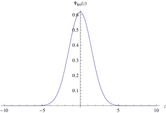
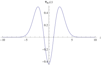
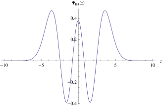
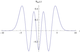
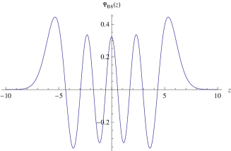
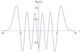
Figure 2: (Normalized) wave functions $\Psi_{B_{2k}}(z)$ for the first six even baryon states.

Table 1 summarizes the mass spectrum for the proton $B=(1,+1/2,0,0)$ and its excitations $B_{X}=(1,+1/2,0,n_{z})$. Note that we have chosen the proton mass $m_{B_{0}}={\widetilde{M}}_{0}=940$ MeV for obvious phenomenological reasons, although strictly speaking the masses are all proportional to $N_{c}$ in the holographic limit $N_{c},\lambda\rightarrow\infty$.

$n$	0	1	2	3	4	5	6	7	8
$m_{B_{n}}$/GeV	0.940	1.715	2.490	3.265	4.039	4.814	5.589	6.655	7.472

Table 1: Some numerical values for the masses of the excited baryon states connected to the proton.

4.3.2 Baryon form factors

According to figure 1, we need to study the interaction of the baryons with (external) photons. This process is represented by the electromagnetic form factors. The Dirac and Pauli form factors were discussed at length in section 2. Here we present our numerical results for the generalized baryon form factors. The infinite sums over vector meson states appearing in the mathematical description of form factors were approximated by including the first 48 vector mesons states in the numerical computations. The wavefunctions $\psi_{2k-1}(z)$ of the vector mesons were discussed at length in ref. [19].
Some numerical results for these quantities are listed in table 2.

$k$	1	2	3	4	5	6	7	8	9
$\frac{m^{2}_{v^{k}}}{M_{\ast}^{2}}$	0.6693	2.874	6.591	11.80	18.49	26.67	36.34	47.49	60.14
$\frac{g_{v^{k}}}{\sqrt{\kappa}M_{\ast}^{2}}$	2.109	9.108	20.80	37.15	58.17	83.83	114.2	149.1	188.7
$g_{v^{k}B_{0}B_{0}}$	5.767	-2.610	0.1902	0.7664	-0.5162	-0.01955	0.2118	-0.08413	-0.05348
$g_{v^{k}B_{0}B_{2}}$	-0.9276	2.4670	-2.6239	1.0560	0.6404	-0.9990	0.2499	0.3848	-0.3049
$g_{v^{k}B_{0}B_{4}}$	0.3655	-1.2608	2.0708	-1.9409	0.6966	0.6716	-0.9855	0.2490	0.4558
$g_{v^{k}B_{0}B_{6}}$	-0.1871	0.7299	-1.4596	1.8556	-1.3815	0.1713	0.8448	-0.8371	0.03738
$g_{v^{k}B_{0}B_{8}}$	0.1091	-0.4595	1.0352	-1.5643	1.5657	-0.7918	-0.3319	0.9318	-0.5634

Table 2: Dimensionless squared masses and decay constants for vector mesons and coupling constants between vector mesons and baryons.

It is interesting to compare our results with experimental data. For the vector mesons, the mass ratios for the first excited states in our framework are $m_{v^{2}}/m_{v^{1}}=2.07$ and $m_{v^{3}}/m_{v^{1}}=3.14$. These results can be compared with the experimental values [52] $(m_{v^{2}}/m_{v^{1}})_{\text{exp}}=1.88$ and $(m_{v^{3}}/m_{v^{1}})_{\text{exp}}=2.20$. For higher excited resonances the discrepancy between our results and the experimental data increases. This should be expected since the spectrum of vector mesons follows a nearly quadratic Regge trajectory in this model [19]. The coupling constant describing the elastic interaction of a $\rho$ meson with a proton can be compared with experimental data. In our framework we obtain $g_{v^{1}B_{0}B_{0}}=5.77$ that is consistent with experimental value $g_{v^{1}B_{0}B_{0}}^{\text{exp}}=4.2-6.5$ [53]. The coupling constant that describes the decay of the resonance $P_{11}(1710)$ into a $\rho$ meson and a proton is $g_{v^{1}B_{0}B_{2}}=-0.93$ in our framework. This value is compatible with the empirical value $|g_{v^{1}B_{0}B_{2}}^{\text{emp}}|=0.6$ obtained from the experimental decay width [54]. There is no available experimental data for higher order couplings.

Using the results for masses and coupling constants we can now easily obtain the Dirac and Pauli form factors for the first few baryon states, as shown in fig. 3. Our results for the elastic form factors of the proton are compatible with the results obtained in chiral soliton models [55]. Again, this should be expected from the fact that baryons in the Sakai-Sugimoto model are holographic representations of four dimensional skyrmions.

Observe that the form factors $F^{D,P}_{B_{0}B_{4}}$ are negative definite. This is not problematic since they will only appear in bilinear combinations in the derivation of the structure functions below, so that the sign will not matter.

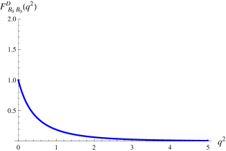
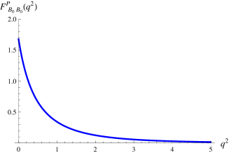
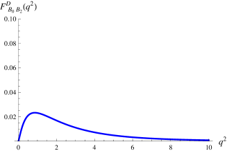
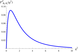
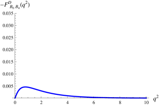
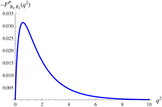
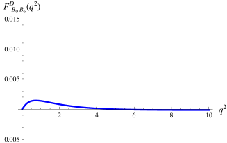
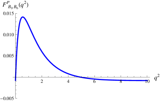
Figure 3: Dirac and Pauli form factors $F^{D,P}_{B_{0}B_{2j}}(q^{2})$ for the first four baryon states. The elastic case corresponds to $j=0$, while $j>0$ yields the transitional form factors. For $j\geq 4$, the numerical errors become relatively large; we can only trust our results for approx. $q^{2}\leq 5\,(\text{GeV})^{2}$.

4.3.3 Helicity amplitudes

In figure 4 we present our numerical results for the helicity amplitudes $|G^{+}_{BB_{X}}(q^{2})|$ and $|G^{0}_{BB_{X}}(q^{2})|$ that have been discussed in section 2.2.2. As before, we study the helicity amplitudes in the large $\lambda$ limit, where the expressions simplify to

$$(G^{+}_{BB_{X}}(q^{2}))^{2} = \left[\frac{q}{\sqrt{2}m_{B}}\left(1+\frac{2}{3}n_{B_{X}}^{2}\frac{M_{\ast}^{2}}{q^{2}}\right)^{1/2}(F^{D}_{BB}(q^{2})+F^{P}_{BB}(q^{2}))\right]^{2}\,,$$ (4.78)

$$(G^{0}_{BB_{X}}(q^{2}))^{2} = \left(1+\frac{q^{2}}{4m_{B}^{2}x^{2}}\right)(F^{D}_{BB}(q^{2}))^{2}\,.$$ (4.79)

The same limitations as for the generalized form factors apply here as well, i.e., the numerical errors become significant for $j\geq 4$ and $q^{2}\geq 5(\text{GeV})^{2}$. Therefore the increase observed in $|G^{+}_{BB_{X}}(q^{2})|$ for $j=3,4$ and $q^{2}$ greater than $4(\text{GeV})^{2}$ may be an artefact of the numerics.

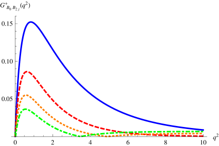
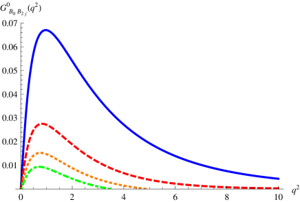
Figure 4: Helicity amplitudes $|G^{+,0}_{B_{0}B_{2j}}(q^{2})|$ plotted versus $q^{2}$ in $(\text{GeV})^{2}$. The transitions from protons to the baryonic final states are labelled by $j$, where $j=1$ (blue, solid), $j=2$ (red, dashed), $j=3$ (orange, dotted) and $j=4$ (green, dotdashed).

Knowledge of the helicity amplitudes $|G^{+}_{B_{0}B_{2j}}(q^{2})|$ is sufficient to determine the helicity amplitudes $|A^{1/2}_{B_{0}B_{2j}}(q^{2})|$. cf. e.g. [45]. The results are visualized in figure 5.

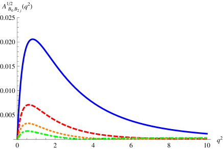
Figure 5: Helicity amplitudes $|A^{1/2}_{B_{0}B_{2j}}(q^{2})|$ plotted versus $q^{2}$ in $(\text{GeV})^{2}$. As before, the transitions from protons to the baryonic final states are labelled by $j$, where $j=1$ (blue, solid), $j=2$ (red, dashed), $j=3$ (orange, dotted) and $j=4$ (green, dotdashed).

The model at hand predicts $A^{1/2}_{B_{0}B_{2j}}(q^{2}\rightarrow 0)=0({\rm GeV})^{-1/2}$, which is consistent with experimental data, cf. e.g., [52, 56]. The experimental result quoted in the PDG summary tables [52] is

$$A_{1/2}(q^{2}=0)=0.009\pm 0.022({\rm GeV})^{-1/2},$$ (4.80)

for the transition between $P_{11}(1710)$ and the ground state. Other theoretical, i.e., quark model predictions are available in the literature, e.g., by Capstick and Arndt et. al. [57, 58],

$$A_{1/2}(q^{2}=0)=0.013({\rm GeV})^{-1/2},$$ (4.81)

for the above mentioned transition.

5 The proton structure functions

5.1 Baryon Regge trajectories in the Sakai-Sugimoto model

Assuming approximate continuity of the mass distribution, we can now approximate the delta distributions in the following way:

$$\sum_{B_{\bf X}}\delta[m_{B_{\bf X}}^{2}-s] \equiv \sum_{n}\delta[m_{n}^{2}-m_{\bar{n}}^{2}]=\int dn\left[\left|\frac{\partial m_{n}^{2}}{\partial n}\right|\right]^{-1}\delta(n-\bar{n})$$ (5.1)

$$= \left[\left|\frac{\partial m_{n}^{2}}{\partial n}\right|\right]_{n=\bar{n}}^{-1}\equiv f(\bar{n}),$$ (5.2)

with the definition

$$s:=-(p+q)^{2}=m_{B_{0}}^{2}+q^{2}(\frac{1}{x}-1).$$ (5.3)

Therefore we have to evaluate the Regge trajectory of the baryon spectrum in order to calculate $\frac{\partial m_{n}^{2}}{\partial n}$. We find (cf. eq. (3.30))

$$\frac{\partial m_{n}^{2}}{\partial n}=\left(\frac{4}{\sqrt{6}}{\widetilde{M}}_{0}M_{\ast}+\frac{4}{3}nM_{\ast}^{2}\right),$$ (5.4)

where ${\widetilde{M}}_{0}$ can be chosen to match, e.g. the proton mass $m_{B_{0}}$ and $n:=n_{z}$.

We obtain an asymptotically quadratic Regge behavior for the baryon resonances in accordance with expectations from the quantized Skyrme model, which is a feature inherited by the Sakai-Sugimoto model, cf. eq. (3.5). However, this is different from the experimentally observed linear behavior of the Regge trajectory. This is a well-known shortcoming of many holographic models of vector mesons and baryons (see for instance [3, 6]). There exist holographic models that exhibit a more realistic linear Regge trajectory by considering a dilaton field in the bulk, e.g. the soft-wall models [42, 43].

5.2 Numerical results

5.2.1 Dependence of $F_{1,2}$ on $q^{2}$ and $x$

It is now possible to extract information about the structure functions $F_{1,2}(q^{2},x)$ employing the following strategy: From the discrete set of baryon mass states and the relation (5.3), we find

$$\Delta m^{2}_{B_{2j}}:=m^{2}_{B_{2j}}-m^{2}_{B_{0}}=q^{2}\left(\frac{1}{x}-1\right).$$ (5.5)

It is possible for each $j>0$ to extract a discrete set of values for $q^{2}$ for a given set of fixed Bjørken parameters, e.g., $x=0.001,\,0.01,\,0.05,\,0.1,\,0.3$. Alternatively, we may calculate a set of values for $x$ for a given set of, e.g., $q^{2}=0.1,\,0.5,\,1,\,2,\,3$ $(\text{GeV})^{2}$. The corresponding values are summarized in table 3.

$j$	$f(\bar{n}=2j)/M^{2}_{\ast}$	$\Delta m^{2}_{B_{2j}}/(\text{GeV})^{2}$	$q^{2}/(\text{GeV})^{2}$	$x$
1	0.233	5.317	$\begin{array}[]{c}0.00532\;\text{for}\;x=0.001\\ 0.0537\;\text{for}\;x=0.01\\ 0.280\;\text{for}\;x=0.05\\ 0.591\;\text{for}\;x=0.1\\ 2.279\;\text{for}\;x=0.3\end{array}$	$\begin{array}[]{c}0.0185\;\text{for}\;q^{2}=0.1(\text{GeV})^{2}\\ 0.0860\;\text{for}\;q^{2}=0.5(\text{GeV})^{2}\\ \;0.158\text{for}\;q^{2}=1(\text{GeV})^{2}\\ 0.273\;\text{for}\;q^{2}=2(\text{GeV})^{2}\\ 0.361\;\text{for}\;q^{2}=3(\text{GeV})^{2}\end{array}$
2	0.144	15.430	$\begin{array}[]{c}0.0154\;\text{for}\;x=0.001\\ 0.156\;\text{for}\;x=0.01\\ 0.812\;\text{for}\;x=0.05\\ 1.714\;\text{for}\;x=0.1\\ 6.613\;\text{for}\;x=0.3\end{array}$	$\begin{array}[]{c}0.00644\;\text{for}\;q^{2}=0.1(\text{GeV})^{2}\\ 0.0314\;\text{for}\;q^{2}=0.5(\text{GeV})^{2}\\ \;0.0609\text{for}\;q^{2}=1(\text{GeV})^{2}\\ 0.115\;\text{for}\;q^{2}=2(\text{GeV})^{2}\\ 0.163\;\text{for}\;q^{2}=3(\text{GeV})^{2}\end{array}$
3	0.0814	30.353	$\begin{array}[]{c}0.0304\;\text{for}\;x=0.001\\ 0.307\;\text{for}\;x=0.01\\ 1.598\;\text{for}\;x=0.05\\ 3.373\;\text{for}\;x=0.1\\ 13.008\;\text{for}\;x=0.3\end{array}$	$\begin{array}[]{c}0.00328\;\text{for}\;q^{2}=0.1(\text{GeV})^{2}\\ 0.0162\;\text{for}\;q^{2}=0.5(\text{GeV})^{2}\\ \;0.0319\text{for}\;q^{2}=1(\text{GeV})^{2}\\ 0.0618\;\text{for}\;q^{2}=2(\text{GeV})^{2}\\ 0.0899\;\text{for}\;q^{2}=3(\text{GeV})^{2}\end{array}$
4	0.0436	54.947	$\begin{array}[]{c}0.0550\;\text{for}\;x=0.001\\ 0.555\;\text{for}\;x=0.01\\ 2.892\;\text{for}\;x=0.05\\ 6.105\;\text{for}\;x=0.1\\ 23.549\;\text{for}\;x=0.3\end{array}$	$\begin{array}[]{c}0.00182\;\text{for}\;q^{2}=0.1(\text{GeV})^{2}\\ 0.00902\;\text{for}\;q^{2}=0.5(\text{GeV})^{2}\\ \;0.0179\text{for}\;q^{2}=1(\text{GeV})^{2}\\ 0.0351\;\text{for}\;q^{2}=2(\text{GeV})^{2}\\ 0.0518\;\text{for}\;q^{2}=3(\text{GeV})^{2}\end{array}$

Table 3: Some values for $q^{2}$ and $x$ according to eq. (5.5).

Lastly, we need to collect some results about the calculation of the isoscalar and isovector magnetic moments for the states under consideration. For the proton and its excited states with $n_{\rho}=0$ and spin up, we find (cf. eqs. (3.16) and (3.32) of [24])

$$\mu^{i}_{I=0}=\frac{1}{4M_{0}}\delta^{3i}\approx 0.842\,\delta^{3i}\,\mu_{B},\quad\mu^{i}_{I=1}=\frac{M_{0}}{3}\frac{\sqrt{5}+2\sqrt{5+N_{c}^{2}}}{2N_{c}}\,\rho^{2}_{\text{cl}}\,\delta^{3i}\approx 3.52\,\delta^{3i}\,\mu_{B},$$ (5.6)

measured in units of the Bohr magneton $\mu_{B}=1/(2m_{B_{0}})$. Here, the mass and size of the classical instanton are $M_{0}=8\pi^{2}\kappa M_{\ast}=558$ MeV and $\rho^{2}_{\text{cl}}=\frac{N_{c}}{8\pi^{2}\kappa M^{2}_{\ast}}\frac{\sqrt{6}}{\sqrt{5}}$, respectively, and we have set $N_{c}=3$ for obvious phenomenological reasons. Sometimes it will be more convenient to utilize magnetic $g_{I}$ factors, which can be defined as follows,

$$\mu^{i}_{I}=\frac{g_{I}}{4m_{B_{X}}}\sigma^{i},$$ (5.7)

where $\sigma^{i}$ are Pauli matrices. The numerical values in the Sakai-Sugimoto model turn out to be

$$g_{I=0}\approx 1.684\,,\qquad g_{I=1}\approx 7.031\,.$$ (5.8)

It is now a fairly straightforward exercise to evaluate the structure functions $F_{1,2}(q^{2},x)$ for the discrete set of values given in table 3. Again, it should be stressed that we work in the large $\lambda$ limit, i.e., we only keep the leading terms in the large $\lambda$, large $N_{c}$ expansion before setting the baryon masses (which are of order $\mathcal{O}(\lambda N_{c})$) to there phenomenological values. The results are presented in figures 6 and 7.

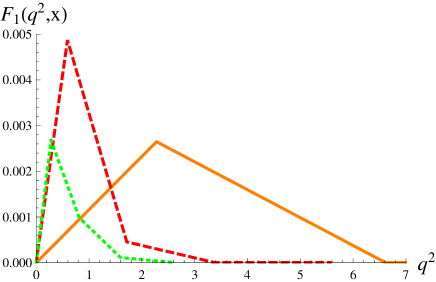
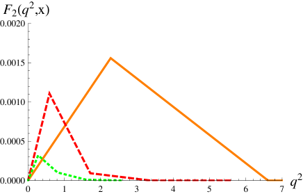
Figure 6: Structure functions $F_{1,2}(q^{2})$ for $x=0.3$ (orange, solid), $x=0.1$ (red, dashed) and $x=0.05$ (green, dotted).

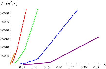
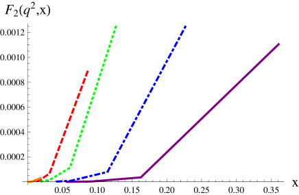
Figure 7: Structure functions $F_{1,2}(x)$ for $q^{2}=3(\text{GeV})^{2}$ (purple, solid), $q^{2}=2(\text{GeV})^{2}$ (blue, dotdashed), $q^{2}=1(\text{GeV})^{2}$ (green, dotted), $q^{2}=0.5(\text{GeV})^{2}$ (red, dashed) and $q^{2}=0.1(\text{GeV})^{2}$ (orange, solid, barely visible) .

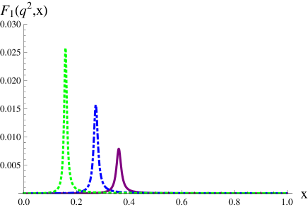
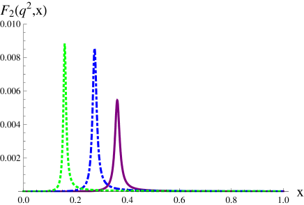
Figure 8: Structure functions $F_{1,2}(x)$ for $q^{2}=3(\text{GeV})^{2}$ (purple, solid), $q^{2}=2(\text{GeV})^{2}$ (blue, dotdashed), $q^{2}=1(\text{GeV})^{2}$ (green, dotted) near the first positive parity resonance $B_{2}$

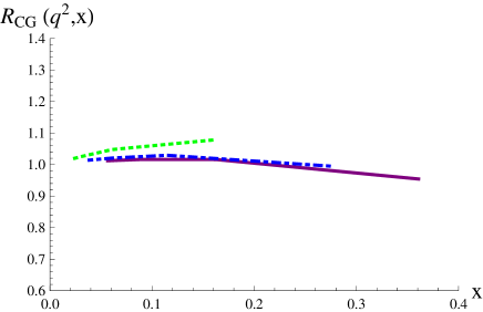
Figure 9: Callan-Gross ratio $R_{\text{CG}}(x)$ for $q^{2}=3(\text{GeV})^{2}$ (purple, solid), $q^{2}=2(\text{GeV})^{2}$ (blue, dotdashed) and $q^{2}=1(\text{GeV})^{2}$ (green, dotted).

5.2.2 Comparing our results with experimental data

The results shown in Figures 6 and 7 indicate that our structure functions $F_{1,2}(q^{2},x)$ seem to be at least two orders of magnitude smaller than what is expected from DIS experimental data (cf., e.g., [52], chapter 16). A possible factor that may contribute to the discrepancy between our results and experimental data is the naive approximation of the Delta distribution that we used in eq. (5.2). Alternatively, we can approximate the Delta distribution by a Lorentzian function [45] :

$$\delta[m_{B_{\bf X}}^{2}-s]\approx\frac{\Gamma_{B_{\bf X}}}{4\pi m_{B_{\bf X}}}\left[(\sqrt{s}-m_{B_{\bf X}})^{2}+\frac{\Gamma_{B_{\bf X}}^{2}}{4}\right]^{-1}\,,$$ (5.9)

where $\Gamma_{B_{\bf X}}$ is the decay width of the resonance $B_{\bf X}$. Identifying the first positive parity resonance $B_{2}$ with the experimentally observed $P_{11}(1710)$ and using the empirical value $\Gamma_{B_{2}}=100\,{\rm Mev}$ we obtain the results for the structure functions shown in Figure 8. Note that the structure functions have improved by an order of magnitude. Unfortunately, we can not follow this procedure for the higher resonances because there are no experimental results available for the decay widths.

The results for the proton structure functions obtained herein are understood to be non-inclusive and only represent a small fraction of possible final states, namely single final state baryons (the excited states of the proton) with spin $1/2$ and positive parity. If we include the contribution from final states with negative parity [59] as well as final states with higher spin and pion production relevant in this kinematical regime, we should get a better picture of the proton structure functions.

5.2.3 Callan-Gross relation

The Callan-Gross relation can be easily studied numerically in this framework in order to check its validity for spin $1/2$ particles. We define the ratio

$$R_{\text{CG}}(q^{2},x):=\frac{F_{2}(q^{2},x)}{2x\,F_{1}(q^{2},x)}\,,$$ (5.10)

and use the numerical results for the structure functions (Figures 6 and 7). The result is shown in Figure 9 and indicates an approximate Callan-Gross relation, i.e. $R_{\text{CG}}\approx 1$ for intermediate values of the Bjorken variable $x$.

6 Conclusions and Outlook

In the present paper we have derived a generalization of the notions of baryon electromagnetic form factors to non-elastic scattering when baryonic resonances with positive parity are produced. Subsequently, we have used the Sakai-Sugimoto model to estimate these form factors in the non-perturbative regime of large $N_{c}$ QCD. We have also estimated the contribution of these form factors to the proton structure functions.

It is important to remark that, in this paper, we have considered the large $\lambda$ limit in the Sakai-Sugimoto model where the description of baryons as solitons is derived from classical small instanton solutions, whose size is of order $\rho^{2}\sim\lambda^{-1/2}$. There may exist $1/\lambda$ corrections that can be dominant at large distances as suggested in a recent analysis [60, 61]. One should also bear in mind the limitations of describing baryons in the large $N_{c}$ limit . Interestingly, in [63] holographic baryons were constructed for the (bottom-up) hard wall model as solitons in an $AdS_{5}$ spacetime with cut-off. These baryons have finite size and have the expected long-distance properties [60]. It would be interesting to investigate baryon resonance production in this model and recent holographic models such as [64, 65] or the recent string models based on the singular [66, 20] and deformed [67, 68] conifold backgrounds. It would be also interesting to estimate the contribution of resonance production in other scattering processes like dilepton production in proton-proton scattering (see [69]).

Appendix A Breit frame for inelastic scattering

Consider the scattering between a virtual photon and a hadron in the hadron rest frame. After two rotations we can set the spatial momentum of the photon to the $x^{3}$ direction, so that

$$p^{\mu} = (m_{B},0,0,0)$$ (A.1)

$$q^{\mu} = (q_{0},0,0,q_{3})\,,$$ (A.2)

and we choose $q_{3}>0$. The virtuality and Bjorken variable in this frame are given by

$$Q^{2}=q_{3}^{2}-q_{0}^{2}\quad,\quad x=-\frac{Q^{2}}{2m_{B}q_{0}}\,.$$ (A.3)

Now we perform a boost in the $x^{3}$ direction so that

$$p^{\prime\mu} = (\gamma m_{B},0,0,-\beta\gamma m_{B})$$ (A.4)

$$q^{\prime\mu} = (\gamma q_{0}-\beta\gamma q_{3},0,0,-\beta\gamma q_{0}+\gamma q_{3})\,.$$ (A.5)

The Breit frame is defined by the condition $q^{\prime}_{0}=0$ so that

$$\beta=\frac{q_{0}}{q_{3}}=\frac{q_{0}}{\sqrt{q_{0}^{2}+Q^{2}}}\quad,\quad\gamma=\frac{\sqrt{q_{0}^{2}+Q^{2}}}{Q}\quad,\quad q^{\prime}_{3}=Q\,,$$ (A.6)

and we arrive at

$$p^{\prime\mu} = (\sqrt{m_{B}^{2}+p_{3}^{2}},0,0,p_{3})$$ (A.7)

$$q^{\prime\mu} = (0,0,0,Q)\,,$$ (A.8)

with

$$p_{3}=-\frac{Q}{2x}\,.$$ (A.9)

References

- [1] P. Kovtun, D. T. Son and A. O. Starinets, “Viscosity in strongly interacting quantum field theories from black hole physics,” Phys. Rev. Lett. 94, 111601 (2005) [hep-th/0405231].
- [2] K. Peeters, M. Zamaklar, “The String/gauge theory correspondence in QCD,” Eur. Phys. J. ST 152, 113-138 (2007). [arXiv:0708.1502 [hep-ph]].
- [3] J. Erdmenger, N. Evans, I. Kirsch, E. Threlfall, “Mesons in Gauge/Gravity Duals - A Review,” Eur. Phys. J. A35, 81-133 (2008). [arXiv:0711.4467 [hep-th]].
- [4] S. S. Gubser, A. Karch, “From gauge-string duality to strong interactions: A Pedestrian’s Guide,” Ann. Rev. Nucl. Part. Sci. 59, 145-168 (2009).
- [5] J. Casalderrey-Solana, H. Liu, D. Mateos, K. Rajagopal and U. A. Wiedemann, “Gauge/String Duality, Hot QCD and Heavy Ion Collisions,” arXiv:1101.0618 [hep-th].
- [6] H. Boschi-Filho and N. R. F. Braga, “AdS/CFT correspondence and strong interactions,” PoSIC 2006, 035 (2006) [hep-th/0610135].
- [7] J. Erlich, “How Well Does AdS/QCD Describe QCD?,” Int. J. Mod. Phys. A 25, 411 (2010) [arXiv:0908.0312 [hep-ph]].
- [8] S. J. Brodsky and F. Guy de Teramond, “AdS/QCD and Light Front Holography: A New Approximation to QCD,” Chin. Phys. C 34, 1 (2010) [arXiv:1001.1978 [hep-ph]].
- [9] U. Gursoy, E. Kiritsis, L. Mazzanti, G. Michalogiorgakis and F. Nitti, “Improved Holographic QCD,” Lect. Notes Phys. 828, 79 (2011) [arXiv:1006.5461 [hep-th]].
- [10] T. Sakai and S. Sugimoto, “Low energy hadron physics in holographic QCD,” Prog. Theor. Phys. 113, 843 (2005) [arXiv:hep-th/0412141].
- [11] T. Sakai and S. Sugimoto, “More on a holographic dual of QCD,” Prog. Theor. Phys. 114, 1083 (2005) [arXiv:hep-th/0507073].
- [12] G. S. Adkins, C. R. Nappi and E. Witten, Nucl. Phys. B 228, 552 (1983).
- [13] M. F. Atiyah and N. S. Manton, Phys. Lett. B 222, 438 (1989).
- [14] H. R. Grigoryan, A. V. Radyushkin, “Form Factors and Wave Functions of Vector Mesons in Holographic QCD,” Phys. Lett. B650, 421-427 (2007). [hep-ph/0703069].
- [15] H. R. Grigoryan, A. V. Radyushkin, “Structure of vector mesons in holographic model with linear confinement,” Phys. Rev. D76, 095007 (2007). [arXiv:0706.1543 [hep-ph]].
- [16] S. J. Brodsky and G. F. de Teramond, “Light-Front Dynamics and AdS/QCD Correspondence: The Pion Form Factor in the Space- and Time-Like Regions,” Phys. Rev. D 77, 056007 (2008) [arXiv:0707.3859 [hep-ph]].
- [17] S. Hong, S. Yoon, M. J. Strassler, “Quarkonium from the fifth-dimension,” JHEP 0404, 046 (2004). [hep-th/0312071].
- [18] D. Rodriguez-Gomez, J. Ward, “Electromagnetic form factors from the fifth dimension,” JHEP 0809, 103 (2008). [arXiv:0803.3475 [hep-th]].
- [19] C. A. Ballon Bayona, H. Boschi-Filho, N. R. F. Braga and M. A. C. Torres, “Form factors of vector and axial-vector mesons in holographic D4-D8 model,” JHEP 1001, 052 (2010) [arXiv:0911.0023 [hep-th]].
- [20] C. A. Ballon Bayona, H. Boschi-Filho, M. Ihl, M. A. C. Torres, “Pion and Vector Meson Form Factors in the Kuperstein-Sonnenschein holographic model,” JHEP 1008, 122 (2010). [arXiv:1006.2363 [hep-th]].
- [21] Z. Abidin and C. E. Carlson, “Nucleon electromagnetic and gravitational form factors from holography,” Phys. Rev. D 79, 115003 (2009) [arXiv:0903.4818 [hep-ph]].
- [22] H. C. Ahn, D. K. Hong, C. Park and S. Siwach, “Spin 3/2 Baryons and Form Factors in AdS/QCD,” Phys. Rev. D 80, 054001 (2009) [arXiv:0904.3731 [hep-ph]].
- [23] D. K. Hong, M. Rho, H. U. Yee and P. Yi, “Dynamics of baryons from string theory and vector dominance,” JHEP 0709, 063 (2007) [arXiv:0705.2632 [hep-th]].
- [24] K. Hashimoto, T. Sakai, S. Sugimoto, “Holographic Baryons: Static Properties and Form Factors from Gauge/String Duality,” Prog. Theor. Phys. 120, 1093-1137 (2008). [arXiv:0806.3122 [hep-th]].
- [25] K. -Y. Kim and I. Zahed, “Electromagnetic Baryon Form Factors from Holographic QCD,” JHEP 0809, 007 (2008) [arXiv:0807.0033 [hep-th]].
- [26] H. R. Grigoryan, T. -S. H. Lee and H. -U. Yee, “Electromagnetic Nucleon-to-Delta Transition in Holographic QCD,” Phys. Rev. D 80, 055006 (2009) [arXiv:0904.3710 [hep-ph]].
- [27] J. Polchinski, M. J. Strassler, “Deep inelastic scattering and gauge / string duality,” JHEP 0305, 012 (2003). [hep-th/0209211].
- [28] C. A. Ballon Bayona, H. Boschi-Filho, N. R. F. Braga, “Deep inelastic scattering from gauge string duality in the soft wall model,” JHEP 0803, 064 (2008). [arXiv:0711.0221 [hep-th]].
- [29] C. A. Ballon Bayona, H. Boschi-Filho, N. R. F. Braga, “Deep inelastic scattering from gauge string duality in D3-D7 brane model,” JHEP 0809, 114 (2008). [arXiv:0807.1917 [hep-th]].
- [30] B. Pire, C. Roiesnel, L. Szymanowski, S. Wallon, “On AdS/QCD correspondence and the partonic picture of deep inelastic scattering,” Phys. Lett. B670, 84-90 (2008). [arXiv:0805.4346 [hep-ph]].
- [31] C. A. Ballon Bayona, H. Boschi-Filho, N. R. F. Braga, M. A. C. Torres, “Deep inelastic scattering for vector mesons in holographic D4-D8 model,” JHEP 1010, 055 (2010). [arXiv:1007.2448 [hep-th]].
- [32] R. C. Brower, J. Polchinski, M. J. Strassler, C. -ITan, “The Pomeron and gauge/string duality,” JHEP 0712, 005 (2007). [hep-th/0603115].
- [33] Y. Hatta, E. Iancu, A. H. Mueller, “Deep inelastic scattering at strong coupling from gauge/string duality: The Saturation line,” JHEP 0801, 026 (2008). [arXiv:0710.2148 [hep-th]].
- [34] C. A. Ballon Bayona, H. Boschi-Filho, N. R. F. Braga, “Deep inelastic structure functions from supergravity at small x,” JHEP 0810, 088 (2008). [arXiv:0712.3530 [hep-th]].
- [35] L. Cornalba and M. S. Costa, “Saturation in Deep Inelastic Scattering from AdS/CFT,” Phys. Rev. D 78, 096010 (2008) [arXiv:0804.1562 [hep-ph]].
- [36] L. Cornalba, M. S. Costa, J. Penedones, “Deep Inelastic Scattering in Conformal QCD,” JHEP 1003, 133 (2010). [arXiv:0911.0043 [hep-th]].
- [37] R. C. Brower, M. Djuric, I. Sarcevic, C. -ITan, “String-Gauge Dual Description of Deep Inelastic Scattering at Small-,” JHEP 1011, 051 (2010). [arXiv:1007.2259 [hep-ph]].
- [38] Y. Hatta, E. Iancu and A. H. Mueller, “Deep inelastic scattering off a N=4 SYM plasma at strong coupling,” JHEP 0801, 063 (2008) [arXiv:0710.5297 [hep-th]].
- [39] C. A. B. Bayona, H. Boschi-Filho and N. R. F. Braga, “Deep inelastic scattering off a plasma with flavour from D3-D7 brane model,” Phys. Rev. D 81, 086003 (2010) [arXiv:0912.0231 [hep-th]].
- [40] E. Iancu and A. H. Mueller, “Light-like mesons and deep inelastic scattering in finite-temperature AdS/CFT with flavor,” JHEP 1002, 023 (2010) [arXiv:0912.2238 [hep-th]].
- [41] Y. Y. Bu and J. M. Yang, “Structure function of holographic quark-gluon plasma: Sakai-Sugimoto model versus its non-critical version,” Phys. Rev. D 84, 106004 (2011) [arXiv:1109.4283 [hep-th]].
- [42] A. Karch, E. Katz, D. T. Son and M. A. Stephanov, “Linear confinement and AdS/QCD,” Phys. Rev. D 74, 015005 (2006) [hep-ph/0602229].
- [43] T. Gutsche, V. E. Lyubovitskij, I. Schmidt and A. Vega, Phys. Rev. D 85, 076003 (2012) [arXiv:1108.0346 [hep-ph]].
- [44] A. V. Manohar, “An introduction to spin dependent deep inelastic scattering,” arXiv:hep-ph/9204208.
- [45] C. E. Carlson, N. C. Mukhopadhyay, “Bloom-Gilman duality in the resonance spin structure functions,” Phys. Rev. D58, 094029 (1998). [hep-ph/9801205].
- [46] H. Hata, T. Sakai, S. Sugimoto, S. Yamato, “Baryons from instantons in holographic QCD,” Prog. Theor. Phys. 117, 1157 (2007). [hep-th/0701280 [hep-th]].
- [47] S. Seki and J. Sonnenschein, “Comments on Baryons in Holographic QCD,” JHEP 0901, 053 (2009) [arXiv:0810.1633 [hep-th]].
- [48] T. H. R. Skyrme, “A Unified Field Theory of Mesons and Baryons,” Nucl. Phys. 31, 556 (1962).
- [49] E. Witten, “Baryons and branes in anti-de Sitter space,” JHEP 9807, 006 (1998) [arXiv:hep-th/9805112].
- [50] E. Witten, “Anti-de Sitter space, thermal phase transition, and confinement in gauge theories,” Adv. Theor. Math. Phys. 2, 505 (1998) [hep-th/9803131].
- [51] H. Boschi-Filho, N. R. F. Braga, M. Ihl and M. A. C. Torres, “Relativistic baryons in the Skyrme model revisited,” Phys. Rev. D 85, 085013 (2012) [arXiv:1111.2287 [hep-th]].
- [52] K. Nakamura et al. [Particle Data Group], “Review of particle physics,” J. Phys. G 37, 075021 (2010).
-
[53]
G. Hohler and E. Pietarinen,
“The Rho N N Vertex In Vector Dominance Models,”
Nucl. Phys. B 95 (1975), 210.
R. Machleidt, “The high-precision, charge-dependent Bonn nucleon-nucleon potential (CD-Bonn),” Phys. Rev. C 63 (2001), 024001; nucl-th/0006014.
F. Gross and A. Stadler, “High-precision covariant one-boson-exchange potentials for np scattering below 350 MeV,” Phys. Lett. B 657 (2007), 176; arXiv:0704.1229. - [54] W. Liu, C. M. Ko and V. Kubarovsky, Phys. Rev. C 69, 025202 (2004) [nucl-th/0310087].
- [55] H. Weigel, Lect. Notes Phys. 743, 1 (2008).
- [56] I. G. Aznauryan et al. [CLAS Collaboration], “Electroexcitation of nucleon resonances from CLAS data on single pion electroproduction,” Phys. Rev. C 80, 055203 (2009) [arXiv:0909.2349 [nucl-ex]].
- [57] S. Capstick, “Photoproduction and electroproduction of nonstrange baryon resonances in the relativized quark model,” Phys. Rev. D 46, 2864 (1992).
- [58] R. A. Arndt, I. I. Strakovsky and R. L. Workman, “Updated resonance photodecay amplitudes to 2-GeV,” Phys. Rev. C 53, 430 (1996) [nucl-th/9509005].
- [59] C. A. Ballon Bayona, H. Boschi-Filho, N. R. F. Braga, M. Ihl and M. A. C. Torres, “Negative parity resonances in the Sakai-Sugimoto model of holographic baryons,” to appear.
- [60] A. Cherman, T. D. Cohen and M. Nielsen, “Model Independent Tests of Skyrmions and Their Holographic Cousins,” Phys. Rev. Lett. 103, 022001 (2009) [arXiv:0903.2662 [hep-ph]].
- [61] A. Cherman and T. Ishii, “Long-distance properties of baryons in the Sakai-Sugimoto model,” arXiv:1109.4665 [hep-th].
- [62] V. S. Kaplunovsky and J. Sonnenschein, “Searching for an Attractive Force in Holographic Nuclear Physics,” arXiv:1003.2621 [hep-th].
- [63] A. Pomarol and A. Wulzer, “Baryon Physics in Holographic QCD,” Nucl. Phys. B 809, 347 (2009) [arXiv:0807.0316 [hep-ph]].
- [64] U. Gursoy and E. Kiritsis, “Exploring improved holographic theories for QCD: Part I,” JHEP 0802, 032 (2008) [arXiv:0707.1324 [hep-th]].
- [65] U. Gursoy, E. Kiritsis and F. Nitti, “Exploring improved holographic theories for QCD: Part II,” JHEP 0802, 019 (2008) [arXiv:0707.1349 [hep-th]].
- [66] S. Kuperstein and J. Sonnenschein, “A New Holographic Model of Chiral Symmetry Breaking,” JHEP 0809, 012 (2008) [arXiv:0807.2897 [hep-th]].
- [67] A. Dymarsky, S. Kuperstein and J. Sonnenschein, “Chiral Symmetry Breaking with non-SUSY D7-branes in ISD backgrounds,” JHEP 0908, 005 (2009) [arXiv:0904.0988 [hep-th]].
- [68] M. Ihl, M. A. C. Torres, H. Boschi-Filho and C. A. B. Bayona, JHEP 1109, 026 (2011) [arXiv:1010.0993 [hep-th]].
- [69] C. A. Ballon Bayona, H. Boschi-Filho and N. R. F. Braga, “Holographic model for dilepton production in p-p collisions,” Nucl. Phys. B 851, 66 (2011) [arXiv:1007.4362 [hep-th]].