SUSY Higgs searches : beyond the MSSM

F. Boudjema¹⁾, G. Drieu La Rochelle¹⁾

1) LAPTh^†, Univ. de Savoie, CNRS, B.P.110, Annecy-le-Vieux F-74941, France

Abstract

The recent results from the ATLAS and CMS collaborations show that the allowed range for a Standard Model Higgs boson is now restricted to a very thin region, if one excludes a very heavy Higgs. Although those limits are presented exclusively in the framework of the SM, the searches themselves remain sensitive to other Higgs models. We recast the limits within a generic supersymmetric framework that goes beyond the usual minimal extension. Such a generic model can be parameterised through a supersymmetric effective Lagrangian with higher order operators appearing in the Kähler potential and the superpotential, an approach whose first motivation is to alleviate the fine-tuning problem in supersymmetry with the most dramatic consequence being a substantial increase in the mass of the lightest Higgs boson as compared to the minimal supersymmetic model. We investigate in this paper the constraints set by the LHC on such models. We also investigate how the present picture will change when gathering more luminosity. Issues of how to combine and exploit data from the LHC dedicated to searches for the standard model Higgs to such supersymmetry inspired scenarios are discussed. We also discuss the impact of invisible decays of the Higgs in such scenarios.

LAPTh-046/11

^†UMR 5108 du CNRS, associée à l’Université de Savoie.

1 Introduction

The impressive 2011 collection of data from the Large Hadron Collider (LHC) provides us with an outstanding insight on many different theoretical models, ranging from the Standard Model to more complex and exotic constructions. Among the latter, supersymmetry is certainly not the least scrutinized. So far no evidence has been found for any new signal in supersymmetry. This leads one to ponder on two complementary issues. On the one hand, in the case of the search for superpartners, the scale of supersymmetry breaking can now be seen to be driven to the TeV range which from the point of view of naturalness puts the original motivation of supersymmetry in jeopardy, even if strictly speaking the argument applies to the third family and the higgsino sector which are directly connected to the Higgs. On the other hand, the current limit on the Standard Model, SM, Higgs cornering its mass in the narrow range between 115 and 140 GeV, where the experimental sensitivity has not enough exclusion power yet and will not probably do so until 2012, is very much compatible with the most simple supersymmetric implementation of the Higgs. Nonetheless since supersymmetry does not seem to be “around the corner” leading to a stronger and stronger tension with the naturalness argument, it has been suggested [1], [2], [3, 4, 5, 6], [7], [8, 9, 10] that new heavy supersymmetric physics can contribute to higher order operators that improve fine-tuning[11, 12, 13]. Another consequence is the possibility, through these new operators, for the lightest supersymmetric Higgs to be much heavier than the usual lightest Higgs of the MSSM (the Minimal Supersymmetric Standard Model). Since the properties and couplings of the Higgses in such BMSSM (Beyond the Minimal Supersymmetric Standard Model) scenarios can be very much modified, it is important to inquire whether such Higgses may be hiding in a wider range than the present narrow range that applies for the standard model Higgs.
A generic analysis for supersymmetric Higgses does not exist since the supersymmetric models are numerous and often lead to different phenomenologies. In addition, the Standard Model Higgs analyses are not straightforward to interpret in a supersymmetric framework, where productions and branching ratios can be greatly enhanced or suppressed. This explains perhaps why the question of excluding the existence of supersymmetric Higgses (and conversely, looking for them if they do not show up in standard model type searches) needs a dedicated study. A common misbelief is to think that because the mass of the lightest Higgs is between 114 GeV and 135-140 GeV, only a few decay modes are allowed. This may be true in the simplest realisation of supersymmetry, the MSSM, but is no longer true for other models, for instance the Next-to Minimal Supersymmetric Standard Model (NMSSM) allows for a lightest Higgs which is much heavier (ref [14]). The 135 GeV upper bound on the lightest Higgs is a feature of the MSSM, not supersymmetry itself. A similar concern is that the lightest Higgs is not necessarily so SM-like : for instance its branching ratio to invisible particles can be important. Thus, hunting the Higgs bosons in the supersymmetric landscape is much of an exploit.
Nevertheless, workarounds do exist. Indeed, most of the difficulty comes from the fact that, if we already know that the MSSM spectrum has to be part of any supersymmetric theory, there are no constraints for additional particles, which means the coexistence of many models. However, if one is only interested in the low energy effects of those particles, one can pursue a model independent approach through an effective field theory, EFT, (see [15] for a review of EFT, among others). This will be the context of the present study : we assume a decoupling between a low energy theory – the MSSM – and new particles, so that the physical effects of the latter will be accounted for by higher-dimensional operators in the supersymmetric potentials. It is well-known (see [1], [2], [3, 4, 5, 6], [7], [8, 9, 10]) that this approach reproduces a wide range of the SUSY Higgs phenomenology. In fact we do not even require a full decoupling between the MSSM spectrum and the new particles, but only a decoupling between the typical energy scale of the Higgs processes at the LHC and the new particles. This approach has the immediate drawback of not accounting for light degrees of freedom, as may exist in the NMSSM with a light singlet for instance : hence some of the BMSSM scenarios will be missed. However, those models require a different study, whereas the effective approach can use the usual MSSM decay channels for Higgses.
While completing this paper an analysis within the same model taking into account LHC data appeared. As we will show our analysis covers ref [10] and goes beyond in considering a few key issues having to do with how to exploit LHC data made in the context of the Standard Model Higgs to models that do not necessarily share the properties of the Standard Model. With the latest ATLAS and CMS combined data (see [16]), we comment on the uncertainties one introduces by attempting to combine data outside the collaborations. In our analysis we cover a larger scan in $\tan\beta$. Moreover, although for most of our study the supersymmetric particles do not play a role, we dedicate a small section to the impact of light enough neutralinos that could contribute to the invisible width of the Higgs. On the theoretical side, we show how one can exploit and extend automated tools such as lanHEP[17, 18] to derive from the superfield formulation the effective Lagrangian in component fields that could easily be fed into matrix element generators.

The article will be organised as follow : in Section 2, we describe the new operators arising in the context of the EFT and their implementation in the aim of studying the Higgs phenomenology. In Section 3 we explain how the Feynman rules of the model are computed which leads to Section 4 which describes how the computation of the relevant observables for Higgs physics is performed. Section 5 is the analysis itself which exploits data from the LHC to derive the latest constraints on the model and will give prospects with the next round of accumulated data. Section 6 outlines our key findings and conclusions. Some technical details of our calculation covering the effective Lagrangian expressed in field components is left to an Appendix.

As shorthand notation, we write $c_{\theta}$ for $\cos\theta$ and similarly for other trigonometric functions.

2 Effective Field Theory

As in any effective field theory, one has to start by defining the low energy theory, and the scale of the heavy spectrum (see [15]). We will do so by fixing the leading order lagrangian to be the one of the MSSM :

$$\mathcal{L}^{(0)}=\mathcal{L}_{MSSM}$$ (1)

and the scale of new physics to be

$$M\sim 1.5\textrm{ TeV}.$$ (2)

The choice of the scale is fixed in order to have a valid effective expansion for relevant observables in the physics under study. Reference[19] catalogues a large number of operators up to dimension-6 within a supersymmetric framework. Here, we are only interested in Higgs phenomenology at colliders where the effect of the high dimension operators is most drastic. A scale above one TeV seems a reasonable choice for Higgs studies even for for LHC energies. Note that the superpartner spectrum can be lower or higher than the scale $M$, without affecting the validity of the effective expansion. The effective expansion is obtained by integrating out the extra heavy particles : the resulting terms are going to enter any of the supersymmetric potentials, namely the Kähler potential $K$, the superpotential $W$, and the susy-breaking potential. Developing the former two, we get :

$$K_{\textrm{eff}} =K^{(0)}+\frac{1}{M}K^{(1)}+\frac{1}{M^{2}}K^{(2)}+O\mathopen{}\left(\frac{1}{M^{3}}\right)$$ (3)

$$W_{\textrm{eff}} =W^{(0)}+\frac{1}{M}W^{(1)}+\frac{1}{M^{2}}W^{(2)}+O\mathopen{}\left(\frac{1}{M^{3}}\right)$$ (4)

The choice of truncating the effective theory at a given order – here at order 2 – is arbitrary and dictated by the required accuracy of the predictions and the computability of the higher orders at the same time. References [8] and [5] have shown independently that the $O\mathopen{}\left(1/M^{2}\right)$ corrections to the Higgs masses are still of the order of 10 GeV, hence we decided to take them into account, but going to third order implied a lot of complications for relatively small changes. For simplicity, and since it should retain most of the contribution to the Higgs observables, we will restrict ourselves to operators involving solely Higgs superfields. Then there is only a handful of those operators in dimension 5 and 6, as was previously shown in [1, 8, 5].

$$\halign to=0.0pt{\relax\global\advance\@IEEEeqncolcnt by 1\relax\begingroup\csname @IEEEeqnarraycolPREr\endcsname#\relax\relax\relax\relax\relax\relax\relax\relax\relax\relax\csname @IEEEeqnarraycolPOSTr\endcsname\relax\relax\relax\relax\relax\relax\relax\relax\relax\relax\endgroup&\relax\global\advance\@IEEEeqncolcnt by 1\relax\begingroup\csname @IEEEeqnarraycolPREC\endcsname#\relax\relax\relax\relax\relax\relax\relax\relax\relax\relax\csname @IEEEeqnarraycolPOSTC\endcsname\relax\relax\relax\relax\relax\relax\relax\relax\relax\relax\endgroup&\relax\global\advance\@IEEEeqncolcnt by 1\relax\begingroup\csname @IEEEeqnarraycolPREl\endcsname#\relax\relax\relax\relax\relax\relax\relax\relax\relax\relax\csname @IEEEeqnarraycolPOSTl\endcsname\relax\relax\relax\relax\relax\relax\relax\relax\relax\relax\endgroup&\global\advance\@IEEEeqncolcnt by 1\relax\bgroup#\egroup&\global\advance\@IEEEeqncolcnt by 1\relax\hbox to\z@\bgroup\hss#\egroup\cr\hfil$\displaystyle W_{\text{eff}}$&\hfil$\displaystyle{}={}$\hfil&$\displaystyle\zeta_{1}\frac{1}{M}\left(H_{1}.H_{2}\right)^{2}$\hfil&{{}\vrule width=0.0pt,height=0.0pt,depth=0.0pt}&0.0pt{\hss{(5)}}\cr\penalty 100\vskip 3.0pt\vskip 0.0pt\cr\hfil$\displaystyle K_{\text{eff}}$&\hfil$\displaystyle{}={}$\hfil&$\displaystyle a_{1}\frac{1}{M^{2}}\left(H_{1}^{\textdagger}e^{V_{1}}H_{1}\right)^{2}+a_{2}\frac{1}{M^{2}}\left(H_{2}^{\textdagger}e^{V_{2}}H_{2}\right)^{2}+a_{3}\frac{1}{M^{2}}\left(H_{1}^{\textdagger}e^{V_{1}}H_{1}\right)\left(H_{2}^{\textdagger}e^{V_{2}}H_{2}\right)$\hfil&{{}\vrule width=0.0pt,height=0.0pt,depth=0.0pt&0.0pt{\hss{(6)}}\cr\penalty 100\vskip 3.0pt\vskip 0.0pt\cr}&+a_{4}\frac{1}{M^{2}}\bigl{(}H_{1}.H_{2}\bigr{)}\left(H_{1}^{{\dagger}}.H_{2}^{{\dagger}}\right)+\>\frac{1}{M^{2}}\left(H_{1}.H_{2}+H_{1}^{{\dagger}}.H_{2}^{{\dagger}}\right)\left(a_{5}H_{1}^{{\dagger}}e^{V_{1}}H_{1}+a_{6}H_{2}^{{\dagger}}e^{V_{2}}H_{2}\right)\vrule width=0.0pt,height=0.0pt,depth=0.0pt{(7)}\cr}$$

where $H_{1},H_{2}$ are the two Higgs superfields in the gauge basis, assuming the hypercharges to be $Y_{1}=-1,Y_{2}=1$. $V_{1},V_{2}$ are the gauge superfields in the representation of $H_{1}$ and $H_{2}$ respectively. Note that we introduced the new parameters $a_{i},\ \zeta_{1}$, that will be referred to as effective coefficients. Those are the remnants of the couplings of the heavy particles to the MSSM spectrum, we will furthermore assume this extra physics to be weakly coupled, ensuring that those coefficients are at most of order one.
So far we have not dealt with the susy-breaking potential, and so what we have are the operators generated by an extra physics that is supersymmetry-conserving. However there is no such a requirement, since susy breaking can occur above or below the scale of extra physics. One natural way to extend our operators to susy-breaking ones is to convert the effective coefficients into spurions (see [5]) :

$$\zeta_{1} \longrightarrow\zeta_{10}+\zeta_{11}m_{s}\theta^{2}$$ (8)

$$a_{i} \longrightarrow a_{i0}+a_{i1}m_{s}\theta^{2}+a_{i1}^{*}m_{s}\overline{\theta}^{2}+a_{i2}m_{s}^{2}\overline{\theta}^{2}\theta^{2}$$ (9)

We have introduced the spurion breaking mass $m_{s}$ (which appears with the Grassman basis vector $\theta$), which for the sake of the effective expansion to hold must be small compared to $M$. This redistributes the operators among the different potentials : $a_{i0}$ operators will be in the Kähler potential, ($\zeta_{10},\ a_{i1}$) in the superpotential, and ($\zeta_{11},\ a_{i2}$) in the soft breaking potential. We take all parameters real. The case of imaginary parameters for the dim-5 operators and its impact on flavour and CP violation is studied in [20]
Foreseeing the physical effects of those operators is rather not intuitive, partly because the scalar potential comes from $F$ and $D$ terms which are much less straightforward than in the MSSM case, and partly because new interactions terms will also appear. To keep track of the new parameters that are introduced, note that the two parameters $\zeta_{10,11}$ are from dim-5 operators whereas the much larger set $\{a_{ij}\}$ stem from dim-6 operators. The lagrangian in terms of fields of a generic supersymmetric theory is given in the Appendix A.1, and we will outline its features in the following.

3 Effective Lagrangian

Whereas the effective theory seems rather simple in its superfields formulation, this is no longer true when looking at the Lagrangian in terms of field components. In comparison, in the MSSM where we also have Kähler potential and superpotential given as superfield functionals :

$$K=K\left(\Phi_{i},\overline{\Phi}_{\overline{j}},e^{V_{n}}\right)\qquad W=W(\Phi_{i})$$ (10)

where $i$ labels the chiral superfields in $\Phi$ and $n$ the different representations of the gauge superfield $V$, the only quantities appearing in the field-component Lagrangian are

$$K_{i\overline{j}}=\partial_{\Phi^{i}}\partial_{\overline{\Phi}^{\overline{i}}}K,\qquad K_{n}=\partial_{e^{V_{n}}}K,\qquad W_{i}=\partial_{\Phi^{i}}W,\qquad W_{ij}=\partial_{\Phi^{i}}\partial_{\Phi^{j}}W$$ (11)

And, from those quantities only $W_{i},W_{ij}$ are non-trivial since it turns out that

$$K_{i\overline{j}}=\delta_{i\overline{j}}\qquad K_{in}=\overline{\phi}_{\overline{i}}.$$ (12)

Beyond the MSSM, not only those simplifications are lost but more derivatives of K and W get involved, as shown in the Appendix. The case of the scalar potential is a good example:

$$V_{\textrm{MSSM}}=-\overline{W_{i}}W^{i}-\frac{1}{2}|K_{n}\;gT^{n}|^{2}\longrightarrow V=-(\overline{\textbf{W}}^{\overline{i}}+\frac{1}{2}K_{\overline{i}kl}\psi^{k}\psi^{l})K_{\overline{i}j}(\textbf{W}^{j}+\frac{1}{2}K_{j\overline{k}\overline{l}}\psi^{\overline{k}}\psi^{\overline{l}})-\frac{1}{2}|K_{n}\;gT^{n}|^{2}$$ (13)

where we have now decomposed the superfields into fields components, that is $\Phi=\binom{\phi}{\psi}$, and the Kähler potential and superpotential are now evaluated on the scalar fields : $K=K(\phi_{i},\overline{\phi}_{j})$ and $W=W(\phi_{i})$.

At this point, it is fair that, though a human processing of the Lagrangian is still feasible, it may easily lead to a large amount of mistakes and should be done again any time one wishes to add another operator, so on the whole does not seem very attractive. For this reason, we decided to use and develop LanHEP , a code dedicated to the computation of Feynman rules particularly handy in the supersymmetric framework ([17, 18]), to derive the field-component Lagrangian. Development was needed since LanHEP did not include higher order derivatives of the Kähler potential and the superpotential. By implementing an extension including all terms of the Lagrangian, together with the truncation of the Lagrangian at a given order of the effective expansion, we had an automated tool to deal with any effective supersymmetric theory.

3.1 Scalar potential

Given the Lagrangian in terms of fields, one can now start to link the initial components of the superfields to the physical fields, on which phenomenological consideration will apply. The first step is to obtain standard kinetic terms for all fields. Indeed, since for electroweak symmetry breaking to occur the Higgs fields acquire non-vanishing vacuum expectation values, the effective expansion will exhibit $K_{i\overline{j}}\neq\delta_{i\overline{j}}$, making kinetic terms no longer trivial. Fortunately, since our new operators only involves Higgs superfields, this affects only Higgs and Higgsinos fields, that we denote by $H_{i}=\binom{\tilde{h}_{i}}{h_{i}}$. Both set of fields will be transformed by the same matrix $P_{\partial}=\sqrt{(K)_{i\overline{j}}}$

$$\binom{h_{1}^{\prime}}{h_{2}^{\prime}}=P_{\partial}\binom{h_{1}}{h_{2}}\qquad\binom{\tilde{h}_{1}^{\prime}}{\tilde{h}_{2}^{\prime}}=P_{\partial}\binom{\tilde{h}_{1}}{\tilde{h}_{2}}$$ (14)

The transformation looks unorthodox at first glance since the two fields do not share the same quantum numbers, but $P_{\partial}$ is non trivial only when the gauge symmetry is broken, which avoids this consideration.
Since all fields are now normalized (from the quantum theory point of view), we can carry on to the next usual step : stabilising the potential. This will fix the values of $v_{1}^{\prime},v_{2}^{\prime}$, the vevs of the $h^{\prime}$ fields (or equivalently $v_{1},v_{2}$ vevs of the $h$ fields). At this point there is another departure from the MSSM : the minimisation constraints can have more than one non-trivial solution : this new minimum will usually be shifted to the heavy scale $M$, whereas the MSSM-like minimum stays at the weak scale. Issues arising when the new minimum becomes the global one, or tunneling features in-between minima have already been discussed in [21], and we will only consider MSSM-like minimum. Naming $V$ the Higgs scalar potential, the minimisation equation simply reads

$$d(V_{\circ}P_{\partial})\,(h^{\prime}\rightarrow v^{\prime})=0\qquad\Leftrightarrow\qquad dV(h\rightarrow v)=0.$$ (15)

where $d$ is the derivative along $\phi$, the vector of Higgs scalar fields. The following step is to find a basis of mass eigenstates, hence diagonalising the mass matrix. In the case of Higgses we write

$$M_{h^{\prime}} = d^{2}(V_{\circ}P_{\partial})\,(v^{\prime})$$ (16)

$$= \left(P_{\partial}\cdot d^{2}V\cdot P_{\partial}\right)_{\circ}P_{\partial}(v^{\prime})$$ (17)

$$M_{h^{\prime}} = \left(P_{\partial}\cdot d^{2}V(v)\cdot P_{\partial}\right)$$ (18)

Since $P_{\partial}$ and $d^{2}V$ are hermitian, $M_{h^{\prime}}$ will be diagonalised by an orthogonal matrix $P$. The relation between the initial fields and the physical fields is then

$$\binom{h_{1}}{h_{2}}=P_{\partial}^{-1}P\binom{h}{H}$$ (19)

in the case of CP-even Higgses. The same applies to CP-odd and charged Higgses, with different $P_{\partial}$ in the charged case (since it is gauge-broken). We will denote the lightest CP even Higgs by $h$ and the heaviest by $H$.

While the expression for $P_{\partial}$ is fairly simple and only includes susy-conserving operator in the Kähler potential (the exact expression is given in Appendix A.2), the mass matrix $M_{h^{\prime}}$ expression is rather cumbersome since all operators are involved and we do not reproduce it here. A similar operation is performed on Higgsinos, and the rest of the spectrum can be diagonalised in the conventional way, leading us to the next computation step.

3.2 Extracting initial parameters from observables

At this stage we have to trade some parameters with experimental data : namely all standard parameters together with the vacuum expectations values, that is

$$g_{1},g_{2},v_{1},v_{2}.$$

Those parameters are fixed by the weak bosons masses, the electromagnetic coupling and the ratio of the vev $t_{\beta}=v_{2}/v_{1}$. The last one being so far undetermined, but can be extracted from decays of the CP-odd Higgs boson, such as $A_{0}\rightarrow\tau^{+}\tau^{-}$. The mass terms of the weak bosons include a contribution from the new operators :

$$M_{Z}^{2} =\frac{1}{2}(g_{1}^{2}+g_{2}^{2})v^{2}\left[1+\frac{v^{2}}{M^{2}}\left(4a_{10}c_{\beta}^{4}+4a_{20}s_{\beta}^{4}+2a_{50}c_{\beta}^{3}s_{\beta}+2a_{60}c_{\beta}s_{\beta}^{3}\right)\right]$$

$$M_{W}^{2} =\frac{1}{2}g_{1}^{2}v^{2}\left[1+\frac{v^{2}}{M^{2}}\left(2a_{10}c_{\beta}^{4}+2a_{20}s_{\beta}^{4}+2a_{30}c_{\beta}^{2}s_{\beta}^{2}+2a_{50}c_{\beta}^{3}s_{\beta}+2a_{60}c_{\beta}s_{\beta}^{3}\right)\right]$$ (20)

We write $v^{2}=v_{1}^{2}+v_{2}^{2}$. We clearly see that some contributions, $a_{10},a_{20}$ and $a_{30}$, lead to $\frac{M_{W}^{2}}{M_{Z}^{2}}\neq\frac{g_{1}^{2}}{g_{1}^{2}+g_{2}^{2}}$, they do not maintain the global $SU(2)$ of the Standard Model Higgs. This particular combination will therefore be very much constrained through indirect electroweak precision measurements.

In order to keep the handy analytic results derived from LanHEP , those equations are solved through Mathematica making use of the effective expansion to perform the extraction linearly. Minimisation of the potential was obtained from the same token. At this point we have successfully obtained the relation from initial parameters and fields to physical observables and fields, so we are ready for the phenomenological study. From all the parameters of the MSSM and the effective expansion, we will use the following subset in the analysis : the mass of the CP-odd Higgs $M_{A_{0}}$ and the ratio of the vevs $t_{\beta}$ from the MSSM, $\zeta_{10},\zeta_{11}$ from the first order contribution and $a_{ij}\ (i=1..6,\ j=0..2)$ from the second order. This adds up to a total of an extra 22 (real) parameters (beside those of the MSSM : $M_{A_{0}},t_{\beta},m_{\tilde{f}},M_{1},\cdots$). This large number of parameters will be an important issue in the numerical analysis and how one scans on this parameter space.

4 Computing observables

Having found the physical fields and computed their masses, extracted the parameters and computed the Lagrangian, we are still far from the complete phenomenology which involves the actual values of the branching ratios and the cross-sections, two quantities not so straightforward to obtain considering that Higgs phenomenology, specially in SUSY models, is plagued with radiative corrections. However since LanHEP did not only provide us with analytic expressions, but also formatted output to phenomenological codes such as CalcHEP[22] and HDecay[23], we merely have to choose which tool to use. So we considered each observable on a case by case basis in order to optimise the precision of the calculation within a reasonable computing time.

4.1 Combining loop and effective expansions

It is a well-known fact that SUSY Higgs phenomenology cannot be separated from loop computations. However, we cannot reach the state of the art prediction obtained in the SM with event generators and multi-loop computation tools starting from scratch with a brand new model. Besides, the accuracy would be unnecessary since we intend to vary freely our effective coefficients in the interval $[-1,1]$. Depending on the observable, some radiative corrections will be computed, as we describe now. First, let us point that we can write any observable as a double expansion, the loop expansion, and the effective one. We will categorise observables as follows :

• Decorrelated expansion. We mean by this that effective couplings and MSSM/QCD loops do not interfere, allowing thus to write $\mathcal{O}=\mathcal{O}^{(0)}+\delta_{\textrm{loop}}\,\mathcal{O}+\delta_{\textrm{eff}}\,\mathcal{O}$, and we can take separately the prediction for $\delta_{\textrm{eff}}\,\mathcal{O}$ from a tree-level code and $\delta_{\textrm{loop}}\,\mathcal{O}$ from an MSSM-dedicated code. This will be the case of masses for instance : $\delta_{\textrm{eff}}\,m$ are taken from the LanHEP output whereas $\delta_{\textrm{loop}}\,m$ are obtained from a spectrum calculator code, namely Suspect [24]. The computation of masses is done as follows : loop-order masses and mixing are computed by the spectrum calculator, and an effective potential is reconstructed from those values (see for example [25]), then the potential coming from higher order terms ($O\mathopen{}\left(1/M,1/M^{2}\right)$) is added and the result is eventually diagonalised. For some observables such as decay to neutralino/charginos, $\delta_{\textrm{loop}}\,\mathcal{O}$ will be neglected.

• Factorisable expansion. This case arises when we can factorise the effective expansion from the loop expansion. That is to say that the scale factor between the tree-level amplitude of the MSSM and the tree-level amplitude in the effective theory is the same as the scale factor between the one-loop amplitudes in both theories, and so on up to the full loop computation, so that this scale factor can safely be applied to the full cross-section. This is equivalent to requiring that both theories have the same K-factor, for the given observable. This is the case of most of the Higgses decay, for instance the partial decay width of the lightest Higgs into $b$ fermions.

  $$\Gamma_{h\rightarrow\overline{b}b}=R_{g_{h\overline{b}b}\ \textrm{eff}}\times\Gamma_{h\rightarrow\overline{b}b\ \textrm{loop}}^{\text{MSSM}}$$ (21)

  where $R_{g_{h\overline{b}b}\ \textrm{eff}}$ is the ratio of the $h\overline{b}b$ coupling in the effective theory to the MSSM one and $\Gamma_{h\rightarrow\overline{b}b\ \textrm{loop}}^{\text{MSSM}}$ is the MSSM partial width.

• Nested expansion. This happens when the loop contribution cannot be neglected, but cannot be factorised either. This is the case for observables such as Higgs decays to photons or gluons. It occurs first at the one-loop level. In those cases, since the effective rescaling of the coupling $g_{h\overline{b}b}$ and $g_{h\overline{t}t}$ are different, the effective scale factor cannot be factorised. Then relations such as eq. 21 do not apply and the computation has to be done with the specific ratio, which usually means modifying some MSSM-dedicated codes such as HDecay[23], as will be detailed later.

At the end of the day, the observables we need are the masses and the product of the production cross-section by the branching ratio to the final state considered : $\sigma\times BR$. Concerning the masses, they are computed with a reasonable accuracy on both sides of the expansion, and in a reasonable time since the effective shift is an analytic formulae, and the loop shift has to be re-evaluated only when changing MSSM parameters.

$$m=m_{\text{loop}}+\delta m_{\text{eff}}$$ (22)

For cross-sections and branching ratios, the experimental results are usually given rescaled from the SM prediction, so in the case of factorisable expansion (with respect to the standard model case) the loop precision is more than sufficient and the computation is straightforward since effective ratios are given as analytic formulas. Examples are decays to fermions or weak gauge bosons :

$$\halign to=0.0pt{\relax\global\advance\@IEEEeqncolcnt by 1\relax\begingroup\csname @IEEEeqnarraycolPREc\endcsname#\relax\relax\relax\relax\relax\relax\relax\relax\relax\relax\csname @IEEEeqnarraycolPOSTc\endcsname\relax\relax\relax\relax\relax\relax\relax\relax\relax\relax\endgroup&\relax\global\advance\@IEEEeqncolcnt by 1\relax\begingroup\csname @IEEEeqnarraycolPREc\endcsname#\relax\relax\relax\relax\relax\relax\relax\relax\relax\relax\csname @IEEEeqnarraycolPOSTc\endcsname\relax\relax\relax\relax\relax\relax\relax\relax\relax\relax\endgroup&\global\advance\@IEEEeqncolcnt by 1\relax\bgroup#\egroup&\global\advance\@IEEEeqncolcnt by 1\relax\hbox to\z@\bgroup\hss#\egroup\cr\hfil$\displaystyle\frac{BR_{h\rightarrow\tau\tau}}{BR_{h\rightarrow\tau\tau\ SM}}=\left(\frac{g_{h\overline{\tau}\tau}}{g_{h\overline{\tau}\tau\ SM}}\right)^{2} $\hfil&\hfil$\displaystyle{}$\hfil&{\vrule width=0.0pt,height=0.0pt,depth=0.0pt}&0.0pt{\hss{(23)}}\cr\penalty 100\vskip 3.0pt\vskip 0.0pt\cr\hfil$\displaystyle\frac{BR_{h\rightarrow WW}}{BR_{h\rightarrow WW\ SM}}=\left(\frac{g_{hWW}}{g_{hWW\ SM}}\right)^{2} $\hfil&\hfil$\displaystyle$\hfil&{\vrule width=0.0pt,height=0.0pt,depth=0.0pt}&0.0pt{\hss{(24)}}\cr}$$

This is also the case of the vector boson fusion, VBF, process, associated vector boson production and heavy quarks associated production.

$$\frac{\sigma_{ZH}}{\sigma_{ZH\ SM}}=\left(\frac{g_{hZZ}}{g_{hZZ\ SM}}\right)^{2}$$ (25)

In the case of nested expansion or MSSM factorisable one, we have used a modified version of HDECAY [23]. This will be used for decays where susy loop contributions are not negligible and also loop induced decays. It is for instance used to compute $\Gamma_{h\to\gamma\gamma}$. Finally, observables where no explicit loop computation was needed have been computed with CalcHEP ([22]) : this is the case for instance of Higgs decay to other Higgses, where the loop correction can be reproduced by an effective potential (see [25]).
Following this choice, several approximations have been made. The most important is the gluon fusion cross-section. As it is a nested expansion case, we started with a modified version of Higlu ([26]), an MSSM-dedicated code. However, the integration over the parton density functions set was an unacceptable lost in time, considering that the effective parameter space was already 22-dimensional. Hence we used the approximation :

$$\sigma_{gg\rightarrow h}=\frac{\Gamma_{h\rightarrow gg}}{\Gamma_{h\rightarrow gg\ SM}}\sigma_{gg\rightarrow h\ SM}.$$ (26)

Similarly if we wanted to consider SUSY loop corrections to the Vector Boson Fusion (VBF), associated vector boson production and heavy quark associated production, we should have used results from MSSM-dedicated code, with the same issue on pdf.
About the branching ratios, using HDECAY did not reproduce the best results for decays into off-shell gauge bosons, but using a more precise tool such as Prophecy4f ([27]) would have raised a lot the computation time, since it goes up to event generation. At the end of the day, production cross-sections were rescaled from the SM predictions (avoiding hence the use of specific codes as Higlu, or codes for VBF), and decays were rescaled from MSSM predictions obtained with HDecay (avoiding the use of Prophecy4f), which allowed for a large gain in computing speed for a very moderate precision loss.

4.2 Accuracy of the effective expansion

The parameters weighing the effective operators must be at most of order 1, if we believe the high energy theory to be weakly coupled. Keeping the leading orders, in our case $1/M$ and $1/M^{2}$, should be sufficient and within the spirit of the effective approach. But even with this requirement we can still be confronted with situations in parameter space where the expansion in $1/M$ can fail. If that is the case then one expects neglected higher order terms such as $O\mathopen{}\left(1/M^{n}\right)$ with $n>2$ to be non negligible. If the inclusion of these higher order terms makes a difference, the expansion is not to be trusted and such configurations of parameters should be discarded. In some situations, for certain observables, the effect of the order $1/M,1/M^{2}$ can be over amplified because the leading order contribution is very small or that there is an accidental suppression that makes the higher order effect important. For instance when $M_{A_{0}}$ is low and $t_{\beta}$ moderate to high, then $h,H$ can get nearly degenerated at zeroth order in the effective expansion. Hence any observable involving $\sqrt{m_{H}^{2}-m_{h}^{2}}$ will have an ill-defined perturbative expansion, since the derivatives of the square root near 0 are infinite.

Our check on the accuracy of the effective expansion is made on the light Higgs mass $m_{h}$, after all the reason for including $O\mathopen{}\left(1/M^{2}\right)$ was because there were non negligible contributions from this order to $m_{h}$. The masses of the CP-even Higgses are computed from the Higgs $2\times 2$ mass matrix $\mathcal{M}$, which in the case where the Lagrangian is truncated at second order, writes as

$$\mathcal{M}_{|2}=\mathcal{M}^{(0)}+\frac{c_{5}}{M}\mathcal{M}^{(5,1)}+\frac{c_{6}}{M^{2}}\mathcal{M}^{(6,1)}+\frac{c_{5}^{2}}{M^{2}}\mathcal{M}^{(5,2)}$$ (27)

Note that $\mathcal{M}^{(0)}$ is the loop corrected mass matrix. To have this concise form, we have used generic names for effective coefficients : $c_{5}$ for the order 5 coefficients $\{\zeta_{10},\zeta_{11}\}$ and $c_{6}$ for the $\{a_{ij}\}$. Now, since $m_{h}$ is obtained by solving a quadratic equation, using eq. 27 leads to a solution that includes contributions up to $O\mathopen{}\left(1/M^{4}\right)$

$$m_{h}=m_{h}^{(0)}+\frac{c_{5}}{M}m_{h}^{(5,1)}+\frac{c_{6}}{M^{2}}m_{h}^{(6,1)}+\frac{c_{5}^{2}}{M^{2}}m_{h}^{(5,2)}+\frac{c_{5}^{3}}{M^{3}}m_{h}^{(5,3)}+\frac{c_{5}c_{6}}{M^{3}}m_{h}^{\binom{5,1}{6,1}}+O\mathopen{}\left(1/M^{4}\right)$$ (28)

So our first check on the effective expansion was to ensure that the $O\mathopen{}\left(1/M^{3}\right)$ terms in eq. 28 were small compared to the $O\mathopen{}\left(1/M^{2}\right)$ terms. We have therefore imposed the condition

$$\left|\frac{\frac{c_{5}^{3}}{M^{3}}m_{h}^{(5,3)}}{m_{h}^{(0)}+\frac{c_{5}}{M}m_{h}^{(5,1)}+\frac{c_{6}}{M^{2}}m_{h}^{(6,1)}+\frac{c_{5}^{2}}{M^{2}}m_{h}^{(5,2)}}\right|+\left|\frac{\frac{c_{5}c_{6}}{M^{3}}m_{h}^{\binom{5,1}{6,1}}}{m_{h}^{(0)}+\frac{c_{5}}{M}m_{h}^{(5,1)}+\frac{c_{6}}{M^{2}}m_{h}^{(6,1)}+\frac{c_{5}^{2}}{M^{2}}m_{h}^{(5,2)}}\right|<0.1$$ (29)

so that points that do not pass this condition were discarded.

Once this algebraic test was passed, we performed another purely numerical test based on the explicit inclusion of an operator of $O\mathopen{}\left(1/M^{3}\right)$. Now the CP-even mass matrix becomes

$$\mathcal{M}_{|3}=\mathcal{M}_{|2}+\frac{c_{5}^{3}}{M^{3}}\mathcal{M}^{(5,3)}+\frac{c_{6}c_{5}}{M^{3}}\mathcal{M}^{\binom{5,1}{6,1}}+\frac{c_{7}}{M^{3}}\mathcal{M}^{(7,1)},$$ (30)

where $c_{7}$ stands for a new operator

$$\mathcal{O}_{7}=\zeta_{3}\left(H_{1}\cdot H_{2}\right)^{3}.$$ (31)

To compute the shift in $m_{h}$, we have run again lanHEP including now the new operator, and requiring the Feynman rules to be computed at order $1/M^{3}$. This being done we could evaluate numerically $\mathcal{M}_{|3}$ and compute the resulting value for $m_{h}$. To do this, we had to assign a value to the $c_{7}$ coefficient. We choose it to be the maximum (in absolute value) of all lower-order coefficients.

$$c_{7}=max\left(|\zeta_{1l}|,|a_{ij}|\right).$$

The additional constraint was set as

$$\left|\frac{m_{h}(\mathcal{M}_{|3})-m_{h}(\mathcal{M}_{|2})}{m_{h}(\mathcal{M}_{|2})}\right|<0.1$$ (32)

Once again, a point failing these two constraints will be discarded. Those two checks are complementary in the sense that the first one ensures only that we do not hit any singular point when computing the Higgs mass, which is essential to use perturbation theory but does not say much about the contribution of higher-orders, while the second constraint is an explicit check that the next order contribution is indeed small enough.

5 Analysis

We have fixed the supersymmetric parameters (except $M_{A_{0}}$ and $t_{\beta}$), since we wanted to focus on the higher-order effects rather than MSSM phenomenology. For the sake of concreteness, we used the $m_{hmax}$ scenario as defined in [28]. All soft masses are set to $M_{{\rm soft}}=1$TeV, $\mu$ and $M_{2}$ are set to 300 GeV, $M_{1}$ is fixed by the universal gaugino mass relation $M_{1}=\frac{5}{3}\tan^{2}\theta_{W}M_{2}\simeq M_{2}/2$, and $M_{3}=800$ GeV ($\cos^{2}\theta_{W}=M_{W}^{2}/M_{Z}^{2}$). All trilinear couplings are set to 0, except for $A_{b}=A_{t}=2M_{{\rm soft}}\frac{\mu}{t_{\beta}}$ that are set to maximise the radiative corrections to $m_{h}$. Maximising $m_{h}$ through purely the MSSM part is not necessary since the new effective operators will enhance the mass more efficiently. We have also set $m_{s}=300$ GeV so that we have

$$\frac{\mu}{M}=\frac{m_{s}}{M}=0.2$$ (33)

Those are, together with $v/M$, the suppression factors of the effective terms. The only free parameters have been varied in the range

$$t_{\beta}\in[2,40]\qquad M_{A_{0}}\in[50,450].$$

Since we are dealing with a large parameter space (22 dimensional), performing a satisfactory scan is a crucial issue. We attempted first a search with random Markov chains, but it ended up to be limited by the frequentist character of the technique : indeed a Markov chain will stay in regions depending on the number of allowed points in it. Because our model exhibits regions that are extremely more populated than others, the Markov chains showed a tendency to stagnate. Besides, we are not interested in the density of points, but in disentangling what lies in the reach of such a generic susy model, and what is incompatible with it. In particular one of our first motivations, in accordance with the main reason for considering such scenarios, is to explore regions where $m_{h}$ is much heavier than what is in the usual MSSM. So after an exploratory random scan we aim at populating regions giving largest values for $m_{h}$. We first carry a blind random scan on all parameters, then we pick up a point exhibiting a large mass and scan again by perturbing around this point. In fact we perturb only around the $O\mathopen{}\left(1/M^{2}\right)$ $a_{ij}$ values rescaling them by a common factor while rescanning on the $O\mathopen{}\left(1/M\right)$ which give the leading order effect in the increase of $m_{h}$. In the scans that we will show later, for $t_{\beta}=2$, we perturb around

$$\begin{array}[]{|cc|cc|cc|cc|}&&a_{10}&0.168605&a_{11}&-0.55814&&\\ a_{12}&0.511628&a_{20}&0.0465116&a_{21}&0.639535&a_{22}&0.802326\\ a_{30}&0.151163&a_{31}&0.744186&a_{32}&0.284884&a_{40}&0.238372\\ a_{41}&0.383721&a_{42}&1.&a_{50}&0.848837&a_{51}&-0.133721\\ a_{52}&-0.732558&a_{60}&0.598837&a_{61}&0.575581&a_{62}&0.331395\end{array}$$

We will refer to this combination as $c_{1}$. We have then carried out reduced scans on the parameter space by randomly choosing a triplet $(x,\zeta_{10},\zeta_{11})$ in the cube $[-1,1]^{3}$, and associate it to the point

$$p=(\zeta_{10},\zeta_{11},x\times c_{1})$$ (34)

This choice strongly relies on the fact that most of the phenomenological change are brought by the order 5 operators, even though the order 6 ones are essential in raising $m_{h}$ further.

5.1 Characteristic features

Figure 1: Features of the BMSSM. In all the plots no experimental constraint has been applied. In the left-top pannel we show the range in the $m_{H},m_{h}$ plane in the BMSSM framework, then on the right the $t_{\beta},m_{h}$ dependence. Plots in the second row all refer to the lightest CP-even Higgs. We first show the cross section for $gg\to h$ normalised to that of the SM as a function of $m_{h}$, then the similar normalised cross section for VBF. The third plot shows the ratio $\sigma_{bb\rightarrow h}/\sigma_{gg\rightarrow h\ SM}$ (this ratio is more relevant than the normalised $bb\rightarrow h$ production since the $b$ quark fusion is rather low in the SM).

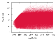
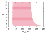
Before applying the constraints coming from collider data, it is worth briefly reviewing what phenomenological changes the BMSSM brings, compared to the SM or the MSSM case. As can be seen in figure 1, the most characteristic feature is the raise in the mass of the lightest CP-even Higgs up to 250 GeV. The largest values can only be reached for low values of $t_{\beta}$, this feature coming from the fact that the shift from dimension 6 operators is suppressed as $t_{\beta}$ increases. Note however that even for $t_{\beta}=40$, the largest value of $m_{h}$ reaches about $160$ GeV, a value larger by more than 20 GeV the corresponding value in the MSSM. We note also some important changes in the production (and the decays) of the light Higgs as compared to the SM case. We note that gluon fusion can be drastically either enhanced or suppressed especially for $m_{h}<160$ GeV. As $m_{h}$ increases the changes in this channel are less drastic, in particular the increase in $gg\to h$ is very moderate. Of course, as we have just seen for $m_{h}>160$ GeV $t_{\beta}$ is low and therefore does not affect much $bbh$ which is enhanced for high values of $t_{\beta}$. This is also clearly displayed in the rate $bb\to h$ where the importance of this channel lies in the region $m_{h}<160$ GeV. In VBF one hardly finds an increase for any Higgs mass, although for $m_{h}<160$ GeV one sees many configurations where the rate can be very small, one still finds scenarios that point to the fact that even for $m_{h}=200$ GeV, the lightest Higgs can be far from being SM-like.

5.2 Indirect constraints from precision electroweak data

We have seen in eq. 3.2 that some operators lead to a breaking of the custodial $SU(2)$ global symmetry. We have implemented the constraints from precision electroweak observables following [29] using data from Ref. [30] and requiring agreement within $2\sigma$. This leads to a very strong constraint on the combination

$$a_{10}-a_{30}t_{\beta}^{2}+a_{20}t_{\beta}^{4}$$ (35)

as can be inferred directly from eq. 3.2.
We do not consider constraint from the flavour sector or even baryogenesis in the BMSSM [31, 32, 33, 20] as one has to specify the details of the matter sector. One can easily bypass possible constraints from this sector by changing the details of the model.

5.3 Constraint from $t\to H^{+}b$

Constraints from not too heavy charged Higgses are imposed exploiting the search of charged Higgs boson in top decays, done by CMS ([34]). The latter explores the channel $t\rightarrow H^{+}b$, $H^{+}\rightarrow\nu\tau^{+}$. Special care was taken in the computation of the branching ratio of $t\rightarrow H^{+}b$, since it can be affected both by QCD corrections and by supersymmetric-QCD corrections. The first have been included using the HDecay code, and the second by including the $\Delta m_{b}$ correction following[35, 36]. To end up with the correction branching ratio, QCD corrections were also taken into accounts for $t\rightarrow W^{+}b$ using HDecay.

5.4 Higgs collider searches: generalities

The Higgs direct searches at the colliders are taken into account by comparing the ratio $\sigma/\sigma_{SM}$ at the 95% CL exclusion value for each analysis by LEP, TEVATRON and the LHC. This is automated via HiggsBounds [37] for LEP, Tevatron and some of the LHC results.
For the neutral Higgs bosons, we must account for the case where $h$ and $H$ get degenerate : in this case the two cross-sections must be added. We define two Higgs bosons to be degenerated when their mass difference is less than 10 GeV for hadron colliders (LHC and Tevatron) and 2 GeV for LEP. The implementation of LHC results from Lepton Photon 2011 had to be done separately, as we show now.

5.5 LHC implementation of the neutral Higgs searches

5.5.1 An “inclusive” analysis

In this first analysis all Higgs search data from from both ATLAS and CMS as presented at Lepton Photon 2011 are used ranging from $1$fb^-1 to 2.3 fb^-1, that we will sometimes refer to for short as $2$fb^-1 data, that is to say :

• $H\rightarrow\gamma\gamma$, done by ATLAS ([38]) and CMS ([39]).

• $VH\rightarrow V\overline{b}b$, done by CMS ([40]).

• $H\rightarrow WW$, done by ATLAS on different final states ($l\nu l\nu$ [41], $l\nu qq$ [42]) and CMS ($l\nu l\nu$ [43]).

• $H\rightarrow ZZ$, done by ATLAS on different final states ($4l$ [44], $2l2q$ [45] and $2l2\nu$ [46]) and CMS ($4l$ [47], $2l2q$ [48], $2l2\nu$ [49] and $2l2\tau$ [50]).

• $H\rightarrow\tau\tau$, done by ATLAS ([51]) and CMS ([52]).

A priori, all these analyses are dedicated to the SM, however we can still try to compare the cross-section we obtain in the BMSSM model with the excluded cross-sections from the collaborations. To this aim we will add all different production cross-sections : gluon fusion ($gg\rightarrow h$), $b$ quark fusion ($bb\rightarrow h$), vector boson fusion (VBF) and associated vector boson production (VH). All SM cross-sections have been taken from the LHC Higgs cross-section working group ([53, 54]) except for the $b$ quark fusion, computed with bbh@NNLO ([55]).
After computing the ratios $\sigma/\sigma^{\text{excl}}$ for each channel, we combine all channels by adding the ratios in quadrature. Moreover, for analyses that exist only in one of the collaborations ($Vb\bar{b}$ in CMS, $WW\to l\nu qq$ ATLAS, $ZZ\to ll\tau\tau$ in CMS), we make up for the lack of the corresponding analysis by including it in our analysis through a scaling factor $\sqrt{2}$ to the corresponding ratio. This approach is followed in Ref.[10] also. The test applies separately to the three neutral Higgses (though in the CP-odd case, some analyses like $H\rightarrow WW$ do not apply) and rejects all points were at least one Higgs fails to pass the test. The excluded inclusive cross section obtained by such an approximation on a SM boson is shown in fig  2.
Since the exact combination of ATLAS and CMS channels in the SM case has recently been published [16], we have presented it on the same plot, fig  2, so one can quantitatively weigh the discrepancy coming from the quadrature sum approximation.

Figure 2: The figure shows the excluded cross sections for the SM Higgs production at the 95% confidence level in the case of the combined analysis performed by the ATLAS and CMS collaborations, exact, compared to the approximate combination we perform based on the quadrature sum, approx.

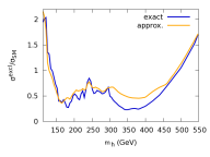
Fig. 2 shows, that apart from the range $300<m_{h}<450$ GeV where all $ZZ$ channels combine, the approximation based on the quadrature sum is well justified. In our model, this range is not reached by the lightest Higgs nor by the CP-odd Higgs which does not couple to vector bosons. Moreover even in the BSSM for $m_{H}>300$ GeV, one is most often in the decoupling limit where the $HWW/HZZ$ is vanishingly small. Therefore for the BSSM the approximate combination should be trustworthy.

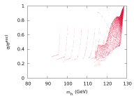
We show in fig. 3 and 4 the allowed points obtained with the analysis we have just described, either in the MSSM and BMSSM cases. In the MSSM case, fig. 3, the light Higgs mass is distributed in between the LEP bound (114 GeV) and the maximum of the radiative corrections (about 130 GeV). We have also plotted here the ratio $R_{\sigma}=\sigma/\sigma_{\text{excl}}$ of each point (it is not necessarily a $h$ signal, but can be any of the three Higgs bosons) against the mass of the lightest Higgs. We notice that this MSSM scenario is largely unaffected by the current results since the ratio between the predicted production rate to the excluded production rate goes down to 0.2, so that one would require an increase by a factor 25 in the luminosity to exclude this particular MSSM model. Models with the highest $m_{h}$ predicted in this model (up to 130 GeV) require much less luminosity increase to be excluded or discovered.

Figure 3: The allowed range in the $m_{h}-m_{H}$ plane for our reference MSSM model is shown in the left panel. The right panel shows the ratio $\sigma/\sigma^{{\rm excl.}}$ as a function of $m_{h}$.

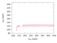
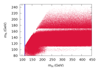
In the case of the BMSSM, the fact that $m_{h}$ can be raised to as high as $250$ GeV changes the picture quite drastically compared to what was allowed before the LHC data (LEP and Tevatron data are included in both sets). Fig. 4 shows that with just about $2$fb^-1 of collected data the $m_{h}-m_{H}$ plane has shrank considerably due to the fact that a rate 2 times smaller than the SM for $m_{h}>160$ GeV is excluded. This shows in particular that $m_{h}>150$ GeV is now excluded. Therefore the main raison d’être of such models that aimed at raising the lightest Higgs mass considerably is now gone. Only an extra $15$ GeV increase for the lightest Higgs compared to the maximal value attained in the usual MSSM framework is still allowed. Therefore the majority of models that survive have $114<m_{h}<150$ GeV, but we do find some regions with smaller values of $m_{h}$.

Indeed, while we find that the heaviest CP-even Higgs is above the LEP limit, $m_{H}>114$ GeV, in the range $114<m_{H}<220$ GeV we find models where the lightest Higgs is lighter than the LEP limit of $114$ GeV, we even find that models with $m_{h}<M_{Z}$ are still possible. In these configurations the lightest Higgs is far from being SM-like. We have seen in fig. 1 that the $hWW$ coupling can be drastically reduced. In this case it is $H$ that picks up almost the totality of the $HWW/HZZ$ coupling, which explains why $m_{H}>114$ GeV (LEP constraint). The configuration with $m_{h}<100$ GeV consists of two separate scenarios as fig. 4 shows. One notices a region that corresponds to $m_{H}>2m_{h}$ starting at $m_{H}=160$ GeV. Here the branching ratio $H\mapsto hh$ can be as high as 0.6, with $h$ decaying almost exclusively to $b$ quarks, makes such scenarios difficult to probe at the LHC. For $114<m_{H}<160$ (GeV), some scenarios are still viable because they correspond to $gg\to H$ that can go down to $50\%$ the value of the SM. Since this reduction is limited to no more than $50\%$, such scenarios will eventually be excluded by a luminosity increase. Other scenarios in this mass range have a $t_{\beta}$ enhanced $bbH$ coupling, which is constrained through $VH\rightarrow V\overline{b}b$ and $H\rightarrow\tau\tau$ which includes $b\bar{b}\to H$ (since the BR to $\tau$ is also significantly enhanced). As the luminosity will increase so will the sensitivity of these last two channels.

Figure 4: BMSSM predictions before (left) after (right) applying the LHC constraints in the $(m_{H},m_{h})$ plane. The vertical blue line shows the LEP SM bound $m_{\Phi}=114$ GeV.

Ref. [10] has very recently carried a very similar analysis. Our results are in very good agreement with theirs apart from the region with $m_{h}<100$ GeV which is more populated in our case. Note that although we carry a similar LHC analysis, we differ in the choice of the MSSM reference point and more importantly in the scan over parameters. One example is the scan in $t_{\beta}$ that is covered uniformly in the range $2$ to $40$ in our case, whereas in Ref. [10] the emphasis was on $t_{\beta}=2$ and $t_{\beta}=20$ with a sparse scan in between. In fact we have verified that our models that survive the actual LHC Higgs constraints have $t_{\beta}$ in the range $5$ to $15$.

5.5.2 Refining the analysis: lessons from a fermiophobic Higgs

The analysis we have just performed, so called inclusive, has exploited results tailored for SM Higgs searches to constrain a model with properties that are quite different from those of the SM as fig. 1 makes evident. Therefore the bias such an approach introduces can be questioned considering that the weight of the different production mechanisms can be very different from those of the SM. An exclusion given on the inclusive $\sigma\times BR$ quantity implicitly assumes that the ratio between each production mode is the same as in the Standard Model, in which case the ratio of exclusive cross-sections is identical to the ratio of inclusive cross-sections. However this assumption breaks down on many BMSSM points. In a nutshell, the applicability of the SM search depends on whether the analysis can differentiate between the different production modes of the Higgs, which would allow to fold in the weight of the different channels in the analysis. Exclusive searches are performed by the collaborations with the aim of selecting a particular sub-channel to enhance sensitivity to a model that would be diluted in a more inclusive search. Analyses for $H\to WW$ that define three categories $H$+0 jet, $H$+1 jet and $H$+2 jet aim for example at enhancing, with the 2-jet, the VBF contribution. The 0-jet subchannel will be quite sensitive to the gluon fusion, since the main part of its inclusive cross-section falls into this category, but very slightly to the VBF. Therefore if one takes a model with gluon fusion dominating all other production modes, like a heavy 4th generation (and to a certain extent the SM), the exclusion will be purely driven by the 0-jet subchannel. If one takes a fermiophobic model, the gluon fusion vanishes and the exclusion is given by the 2-jets subchannel. It is clear that the signal obtained in the 4th generation model or the fermiophobic model with the same inclusive cross-section (combining 0,1,2-jet) is not the same and will not lead to the same exclusion limits. In such a case one would then have to scale the cross-section reweighted by the efficiency of each mode ($gg$, VBF, …) that contributes to the same inclusive final state, that is to say computing the ratios that quantify the exclusion power

$$R_{\text{incl}}=\frac{\sigma}{\sigma_{SM}}=\frac{\sum_{i}\sigma_{i}}{\sum_{i}\sigma_{SM\ i}}\quad\longrightarrow\quad R_{\text{excl}}=\frac{\sum_{i}\sigma_{i}\epsilon_{i}}{\sum_{i}\sigma_{SM\ i}\epsilon_{i}}$$ (36)

where $i$ runs over the production mode (gluon fusion, VBF and so on) and $\epsilon_{i}$ is the associated efficiency. We will then compare with the excluded value. One can estimate the difference between the two approaches of eq. 36 by plotting the excluded cross-section of different models for a single search.

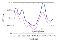
For $H\to\gamma\gamma$ a category with a harder $p_{T}^{\gamma\gamma}$ favours Higgs production through VBF or vector boson associated production over $gg$ induced where the Higgs has a smaller $p_{T}$. Such separation could very useful and efficient in, again, the case of a fermiophobic Higgs whose $gg$ induced cross section is vanishing, in sharp contrast to the SM Higgs. This particular model can be used as an example, though perhaps extreme since one important SM channel is absent, to quantify the difference one gets from an inclusive (in this case merging all $p_{T}^{\gamma\gamma}$ regions) compared to an exclusive search or exclusion limit for each $p_{T}^{\gamma\gamma}$ region. Such an approach has been performed by CMS [39]. In that analysis the classification is done according to $p_{T}^{\gamma\gamma}>40$ GeV for enhancing the fermiophobic signal over background. If we consider the inclusive cross-section, in this case no $p_{T}^{\gamma\gamma}$ separator, to set the limits on $\sigma\times BR$, the limit would be the same in any model since it would only be computed from the measured number of events, the predicted background and its systematics (if we neglect theoretical systematics). Using the exclusive method based on the $p_{T}^{\gamma\gamma}>40$ GeV as a separator gives a much more powerful limit, though model dependent limit as shown in fig. 5. Unfortunately CMS does not provide separate exclusion limit for each region in $p_{T}^{\gamma\gamma}$. In fact CMS gives the values obtained for $\sigma^{\text{excl}}$ using both models, in the merged (inclusive) and the split (exclusive) analyses for $m_{h}=120$ GeV.

$$\begin{array}[]{ccc}&\sigma_{\text{merged}}^{\text{excl}}(pb)&\sigma_{\text{split}}^{\text{excl}}(pb)\\ \text{SM}&0.1308&0.1104\\ \text{fermiophobic}&0.1303&0.0696\\ \end{array}$$

One notices first that the values of $\sigma_{\text{merged}}^{\text{excl}}$ are nearly the same in the two models, which emphasize the fact that inclusive limits are more model independent than exclusive ones. We note that the gain in the SM is approximately 20%, and in the fermiophobic model nearly 50%. Therefore applying this $20\%$ correction to the inclusive analysis mimics the effect of a more refined two-region analysis.

Figure 5: The panel on the left shows the SM and fermiophobic excluded cross-sections in the $H\rightarrow\gamma\gamma$ CMS analysis, these plots are extracted from Ref. 5. Cross sections are given in picobarns. On the right is shown the relative difference between fermiophobic and SM analyses, in percent units.

This mean that if one had used the SM limit with the inclusive approach in the context of a fermiophobic Higgs, one would have lost a factor 2 in sensitivity compared to a more refined optimised exclusive analysis.
Unfortunately at present the details of the analyses performed by ATLAS and CMS do not provide all the needed information and efficiencies that we require for an exclusive approach. At present in a phenomenological analysis like ours the best that can be done is to simulate the experimental analysis through a Monte-Carlo with the caveat that some detector issues contributing to the efficiencies may be lost.

5.5.3 Refining the analysis

Improving the analysis means that we will attempt to exploit those channels where separators leading to exclusive observables have been conducted. Of course the situation is different from the case of the fermiophobic model in the $\gamma\gamma$ signature where only one channel is selected. Moreover the fermiophobic model is well defined, $gg\to h$ cross section is vanishing. In the scans we perform in the BMSSM case one is in fact considering many models where a given Higgs mass, $m_{h}$, corresponds to models with very different properties. Let us first go through all the channels we have used in the previous analysis and comment on how one could, for some of them, take into account the exclusive nature of a particular final state.

• $VH\rightarrow V\overline{b}b$. In this case there is only one production mode, the vector boson associated production. Although it is strictly speaking two modes, the $Z$ and $W$, the scaling factor from the SM is nearly exactly the same, which simplifies the analysis. Here we can safely use inclusive cross-sections, since we only rescale the SM production.

• $H\rightarrow\tau^{+}\tau^{-}$. This channel is of interest in the MSSM and BMSSM for high $t_{\beta}$. $H$ is produced either through $gg$ fusion of $bb$ fusion. The ATLAS analysis ([51]) presents excluded cross-sections for each of these two production modes. This is most useful when analysing a new model as we can weigh each sub-channel separately. This piece of information is extremely helpful since it gives the efficiency in a very handy way : one has just to compute the ratio of each production cross section to its excluded value, sum them and compare to 1. Indeed as we deal with a counting experiment, this is adding events from each production mode and compare with the excluded number of events, which, in the approximation of no theoretical systematics, is justified.

• $H\rightarrow ZZ\rightarrow 4l$. Unlike the $WW$ signature where an analysis including 0-jet, 1-jet and 2-jet is performed, for the $ZZ$ channel one only has at the moment a fully inclusive analysis.

• $H\rightarrow\gamma\gamma$. We have just seen in the fermiophobic Higgs search that CMS, and similarly ATLAS, divide the phase space according to $p_{T}^{\gamma\gamma}$ that allows to give different exclusion limits if one assumes a fermiophobic model compared to the SM. As we have just argued, the efficiencies in the two regions are not given. Our procedure here is to correct the inclusive analysis of CMS [40] by $20\%$ to recover the fully inclusive limit. Although this scaling was derived for $m_{h}=120$ GeV, considering the narrow range of the $\gamma\gamma$ channel we assume this scale factor to be roughly constant. This is a conservative approach, but a precise analysis requires the exclusion cross section for each subchannel (here the $p_{T}^{\gamma\gamma}$ regions) and the efficiencies of each mode.

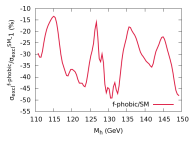
• $H\rightarrow WW\rightarrow l\nu l\nu$. Both ATLAS and CMS split the channel according to the number of recorded jets, which allow to gain sensitivity to specific production modes ($gg\to H$ or VBF). Fortunately enough, ATLAS provides exclusion limits for the 0-jet and 1-jet subchannel (and should soon provide the 2-jet bin). Providing the 2-jet that would select the VBF would be extremely useful. Once again though the weight of the 0-jet and 1-jet in the ATLAS analysis are folded in, these weights are not provided. Simulating the ATLAS analysis one could in principle calculate these weights or efficiencies. We have run PYTHIA for a SM Higgs boson through gluon fusion, VBF or $b$ quark fusion and extracted the efficiency of each production mode. Although this may seem far too naive since full detector simulation is not applied we are only interested in the relative efficiencies, say the ratio between the VBF and gluon fusion. One expects that a full detector simulation does not affect these ratios much. The ratios we calculated were validated by the ATLAS collaboration. $b$ fusion could not be checked since it is not included in a SM Higgs analysis. We were then able to fold in these ratios witin a refined exclusive analysis. We show in fig 6 the relative difference between the inclusive and exclusive, defined in eq 36. This relative correction is mainly positive, up to $30$% which can be traced back to the fact that the $b$ fusion efficiency is higher than the gluon fusion one.

To summarise we see that for the moment, the refinement concerns only two channels and may seem a modest improvement, but it is important to send a signal and a request to the collaborations so that details of the analyses with the weight and efficiencies of all channels and sub-channels be released. It is important to stress that what we call the refined analysis is our approach to arrive at what we think is a better treatment of such models, nonetheless with the inclusive analysis this allows to compare and quantify the assumptions. It should also be clear that the refined analysis does not necessarily mean that it is more constraining than the inclusive one. Before turning to the final results taking into account these refinements and in order to understand their impact when scanning over a large set of parameters, we compare the exclusion power in terms of the inclusive approach compared to the refined analysis, eq. 36, applied to the heaviest CP-even Higgs for illustration. The comparison is shown in fig. 6 corresponding to the luminosity $2$fb^-1 (Lepton-Photon 2011). Note that we only display values with $R_{{\rm incl}}<1,R_{{\rm excl}}<1$ corresponding to models that are still viable. When the luminosity increases, the condition $R_{{\rm incl}}<1,R_{{\rm excl}}<1$ can be read from the plot, but would correspond to smaller $R$ values.

Figure 6: We show the exclusion power based on the inclusive analysis compared to the refined analysis, see text, applied to searches for the heaviest CP-even Higgs

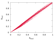
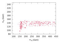
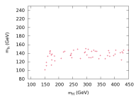
The figure shows that there is, unfortunately, little spread around $R_{{\rm incl}}=R_{{\rm excl}}$, the largest differences attaining about $20\%$ for $R<0.3$. A scan over the entire parameter set, taking all constraints on all Higgses, showed practically not much difference between the refined and inclusive approach when projected on the $m_{h}-m_{h}$ plane. So we will not show such plots. However to illustrate that the two analyses do exclude different sets of models, we have generated a well chosen subset of models and passed them through the two analyses, inclusive and refined. In this (biased) chosen subset of models, we see in fig. 7 that the refined analysis excludes many more models. Had we performed a full scan, the differences in the projection on the plane $m_{h}-m_{H}$ will hardly be visible.

Figure 7: Taking a small subset of models, we apply an inclusive analysis, left panel, and compare it to the result of a refined analysis, right panel.

5.6 Expectations with higher luminosities

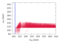
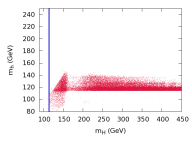
The LHC is running wonderfully. We have seen that the first set of data on Higgs searches released this summer has already put severe constraints on models such as the BMSSM. It is therefore very tempting to make projections with an increase of luminosity. Indeed ATLAS and CMS will very soon release data with $5$fb^-1. We show in fig. 8, by simply rescaling our refined analysis by the luminosity factor, how the picture changes as the luminosity is increased from $5$, $10$ to $15$fb^-1.
Compared with the limits based on the released data with $2$fb^-1, we notice first that as the luminosity increases the upper limit on $m_{h}$, which sits now at $150$ GeV, decreases gradually affecting first those models associated with $m_{H}>300$ GeV. Already with $10$fb^-1, there are practically no models with $m_{h}>140$ GeV for $m_{H}>300$ GeV. With $15$fb^-1 only very few models with $m_{H}<150$ GeV remain. With this luminosity the number of models with $m_{h}<114$ GeV is also drastically reduced and at $15$fb^-1 they are practically all gone if $m_{H}>150$ GeV. At this luminosity, though much reduced, the space with $m_{h}<114$ GeV and $m_{H}<150$ GeV is still there. This said at this luminosity, if the density of surviving models is any indicator for the likelihood of a model, we see that there is a concentration of models within a thin layer with $114<m_{h}<120$ GeV when $m_{H}>250$ GeV, although of course many models still survive with $m_{h}$ up to $m_{h}=140$GeV.

Figure 8: Remaining parameter space when the luminosity increases. The top panel shows the expectation for 5fb^-1. In the second row the panel on the left is for 10fb^-1and the one on the right is for 15fb^-1.

5.7 Higgs decays to invisibles

We present now the preliminary results of the consequence of the Higgs decaying to invisible particles. Despite numerous advantages, the $m_{h\ max}$ scenario does not cover the full diversity of the MSSM nor the BMSSM, in particular it does not cover cases where the Higgs can decay to neutralinos, in particular the lightest ones. The latter are good dark matter candidates and therefore these decays of the ligtest Higgs are into invisibles. In order to have a sufficient branching ratio to the neutralino one must have a neutralino which is light enough, $M_{\tilde{\chi}^{0}_{1}}<m_{h}/2$. We do not wish here to conduct a thorough analysis of the BSSM higgses into invisibles and review all the constraints from dark matter, we leave this to a more focused study. Dark matter issues within the BSSM taking into account the dim-5 operators were conducted in [58, 59, 60, 61]. Though succinct our implementation includes dim-6 operators automatically. In the recent approach of [62] which can be related to a BSSM implementation, decays are into invisible light scalars.

In this exploratory study we consider $M_{\tilde{\chi}^{0}_{1}}<80$ GeV. In order to achieve this while taking into account LEP limits on the chargino mass, such light neutralino are dominantly bino-like. However in order to couple to the Higgs efficiently there must be a higgsino component that is not too negligible, see for example [63]. One should therefore have $M_{1}$, the bino mass, and $\mu$ not too far apart. We will set $M_{1}=50$ GeV to have a light neutralino and $\mu=200$ GeV to have enough mixing. The alert reader will have noticed that this value of $\mu$ is smaller than what we have been using so far. In order that our previous results are unaltered so that we can compare with what an invisible decay brings, one should remember that the phenomenology without invisibles is unchanged if one keeps the ratios $\mu/M,\ m_{s}/M$, that governs the effective expansion in $1/M$, identical to what was stated in eq. 33.

Figure 9: Higgs decays to invisible neutralinos. The first graph shows the branching ratio of the light Higgs to the lightest neutralinos, see text for details on the parameters of the neutralinos. In the second row, the first panel shows the allowed $m_{h}-m_{H}$ space taking into account the present LHC constraint ($2$fb^-1). The graph on the right is for a luminosity of $15$fb^-1.

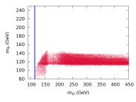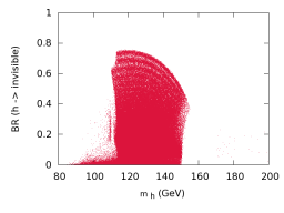
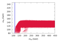
Fig 9 shows the branching ratio of the light Higgs to the lightest neutralinos. Between $m_{h}=120$ GeV and $m_{h}=150$ GeV, the branching ratio is substantial ranging from $~{}80\%$ to $40\%$ for $m_{h}=150$ GeV, at which point it drops precipitously to almost $0\%$ because of the opening of the $WW$ channel. When the branching into the lightest neutralinos is large it reduces all the usual branchings and leads to a much reduced sensitivity of the Higgs signal. Fig. 9 shows how the picture changes when decays to invisibles are allowed. With the current data ($2$fb^-1) it is difficult to see that changes have occurred. This is not surprising since our invisible scenario can only cut in the $m_{h}$ range $120-150$ GeV . With the present luminosity this range is still very much viable even without Higgs decays as we have seen. With the luminosity at $15$fb^-1, we clearly see the damaging effect of the invisible decays. More models with Higgs masses up to $m_{h}=140$GeV survive compared to the case where no invisible Higgs decays are allowed.

5.8 Update from the preliminary results of the LHC with 5 fb^-1

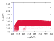
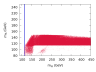
A week after our paper was made public, the ATLAS and CMS collaborations released the updates of some of their Higgs analyses with $4.6$fb^-1 to $4.9$fb^-1 (see [64, 65] for combinations of the different channels in each experiment). Since these results are now available, we could update our analysis. The released data point to an excess in some channels for $m_{h}\sim 124-126$GeV in particular in the case of ATLAS where taking into account the look elsewhere effect the global significance of the effect is $2.4$ standard deviations, thus not enough to claim any discovery. In this section we therefore only consider the no signal interpretation and apply the 95% exclusion limit for those channels that have been reanalysed by ATLAS and CMS. Compared to the full listing given in section 5.5.1 the update includes i) for CMS: $\gamma\gamma$, $V\overline{b}b$, $\overline{\tau}\tau$, $WW\to l\nu l\nu$, $ZZ\to 4l$ ii) for ATLAS: $\gamma\gamma$, $ZZ\to 4l$, $WW\rightarrow l\nu l\nu$. We have kept the same data set corresponding to $1$-$2.1$fb^-1 luminosity for the rest of the list (with the “inclusive” analysis). This is to be compared to our projection for $5$fb^-1 where we applied a luminosity rescaling on all the channels of the list. Our analysis of the update is shown in fig. 10 in the plane $m_{h}-m_{H}$ . To guide the eye and make the comparison easy, the figure also shows the results based on the rescaling of all the channels. We see little difference, the analysis based on a full rescaling of all channels is, naturally, slightly more restrictive.

Figure 10: Allowed range for $m_{h}$ and $m_{H}$ taking into account the updated ATLAS and CMS data with $4.6-4.9$ fb^-1(left) compared to our previous analysis where a luminosity rescaling to $5$ fb^-1 is applied to all channels(right), refer to the text for more details.

6 Conclusions

It is quite clear by now that Higgses in supersymmetric models that go beyond the MSSM are very much constrained by the LHC searches, even though the primary goal of those searches is the Standard Model Higgs. We have first shown that the higher-order terms appearing in the effective Lagrangian alter the Higgs phenomenology quite significantly, in particular by raising the lightest Higgs mass to values up to 250 GeV. This feature alone was the main motivation of the BMSSM. We have shown that with the advent of the LHC and the data collected so far, experiments no longer allow a lightest supersymmetric Higgs to have a mass beyond $150$ GeV even in these BMSSM set ups and even if we allowed for decays into invisibles as provided by the lightest neutralinos. With the increase of the luminosity most of the remaining models at $15$fb^-1 are within a thin layer in lightest Higgs mass, with $114<m_{h}<140$ GeV with a concentration around $m_{h}\sim 120$GeV, apart from an island with $m_{h}<100$ GeV for $m_{H}$ low enough, $m_{H}<150$GeV. Invisible decays allow more models with $m_{h}\sim 140$GeV. Within this picture, set in terms of exclusions, and with $15$fb^-1 of data, a similar conclusion in terms of masses applies to the MSSM, the BMSSM lightest Higgs is allowed to be less than about $10$GeV heavier that what it can be in the MSSM, whereas before the advent of the LHC masses for the lightest BSSM Higgs up to $250$GeV were possible. Still the phenomenology of the two models is quite different. Although our philosophy in this paper has been towards constraining the BMSSM models in the pessimistic prospect of no Higgs signal, it would be very interesting to revisit the models in case of a signal. If the density of allowed models that we have found is any indication for where a possible signal may be hiding and if the possible slight excess in the latest data from the LHC is confirmed, it would be extremely interesting to check whether the signals are better described by a BMSSM Higgs with $m_{h}=125$ GeV and what the properties of the latter are. Could one always tell it apart from a MSSM one or even a standard model one? We have not addressed this issue here. What we have addressed however, though perhaps partially, is how to exploit LHC results made for the SM Higgs in the context of other models that can have quite different properties. We have made a request that the collaborations should provide more details about the weight of the different sub-channels that are used in their analyses.

Acknowledgments
We would like to thank Geneviève Bélanger for interesting discussions throughout the study, Filip Moorgat for providing us more insight on the CMS analyses. We also wish to thank Nicholas Berger, Marta Felcini, Dmytro Kovalskyi, Biswarup Mukhopadhyaya, Sasha Nikitenko, as well as the participants in the Higgs working group at the workshop Physics at TeV Colliders in Les Houches in June 2011. Finally we acknowledge the exchanges with Marcela Carena clarifying some points concerning the analyses in Ref.[10]. This work is part of the French ANR project, ToolsDMColl BLAN07-2 194882 and is supported in part by the GDRI-ACPP of the CNRS (France).

A Appendix

A.1 Field-component Lagrangian

$$\begin{split}\mathcal{L}_{K}\ =\ &-(\overline{\textbf{W}}^{\overline{i}}+\frac{1}{2}K_{\overline{i}kl}\psi^{k}\psi^{l})K_{\overline{i}j}(\textbf{W}^{j}+\frac{1}{2}K_{j\overline{k}\overline{l}}\psi^{\overline{k}}\psi^{\overline{l}})-\frac{1}{2}|K_{n}\;gT^{n}|^{2}\textbf{W}_{W}^{\,-1}\hskip 28.45274pt\textrm{scalar potential}\\ &+iK_{in}\;\partial_{\mu}\phi^{i}\;(gv)^{n\ \mu}\hskip 28.45274pt\textrm{gauge-scalars interaction}\\ &+K_{nm}\;(gv)^{n\ \mu}\;(gv)^{m}_{\ \mu}+K_{n}\;(gv)^{n\ 2}\hskip 28.45274pt\textrm{gauge-gauge-scalars interaction}\\ &+\frac{1}{2}K_{i\overline{j}}\;\partial_{\mu}\phi^{i}\;\partial^{\mu}\overline{\phi}^{\overline{j}}\hskip 28.45274pt\textrm{scalars derivatives}\\ &+i\frac{\sigma^{\mu}}{2}K_{i\overline{j}}\;\partial_{\mu}\psi^{i}\;\overline{\psi}^{\overline{j}}+\frac{1}{2}\textbf{W}_{ij}\;\psi^{i}\;\psi^{j}+i\frac{\sigma^{\mu}}{2}K_{ij\overline{k}}\;\partial_{\mu}\phi^{i}\;\psi^{j}\;\overline{\psi}^{\overline{k}}\hskip 28.45274pt\textrm{fermion-fermion-scalars}\\ &+i\sqrt{2}K_{in}\;\psi^{i}\;(g\lambda)^{n}+\sigma^{\mu}K_{i\overline{j}n}\;\psi^{i}\;\overline{\psi}^{\overline{j}}\;(gv)^{n}_{\ \mu}\hskip 28.45274pt\textrm{gauge-fermion-scalars interaction}\\ &+\frac{1}{4}K_{ij\overline{k}\overline{l}}\;\psi^{i}\;\psi^{j}\;\overline{\psi}^{\overline{k}}\;\overline{\psi}^{\overline{l}}\hskip 28.45274pt\textrm{4 fermions-scalars interactions}\\ &+\textbf{W}_{W}\,\left(-\frac{1}{4}F_{\mu\nu}F^{\mu\nu}-i\lambda\sigma^{\mu}D_{\mu}\overline{\lambda}\right)\hskip 28.45274pt\textrm{gauge interactions}\\ &+\mathcal{L}_{SSB}\\ &+h.c.i.n.\end{split}$$ (A.1)

A.2 Kinetic rescaling

Because of the kinetic Lagrangian for Higgs fields is non standard

$$\mathcal{L}_{\textrm{kinematics}}=d\phi^{\dagger}K_{2}d\phi+i\overline{\psi}K_{2}d\!\!\!/\,\psi$$ (A.2)

we have to rescale the Higgs field in the following way.

$$\binom{h_{1}^{\prime}}{h_{2}^{\prime}}=P_{\partial}\binom{h_{1}}{h_{2}}\qquad\binom{\tilde{h}_{1}^{\prime}}{\tilde{h}_{2}^{\prime}}=P_{\partial}\binom{\tilde{h}_{1}}{\tilde{h}_{2}}$$

with $P_{\partial}=\sqrt{K_{i\overline{j}}}$. This quantity is straightforward to obtain from the effective Kähler potential 3, and is the following, in terms of physical inputs

$$P_{\partial}=1-\frac{1}{1+t_{\beta}^{2}}\frac{v_{0}^{2}}{M^{2}}\begin{pmatrix}4a_{10}+4t_{\beta}a_{50}+(a_{30}+a_{40})t_{\beta}^{2}&a_{50}+t_{\beta}(a_{30}+a_{40})+t_{\beta}^{2}a_{60}\\ a_{50}+t_{\beta}(a_{30}+a_{40})+t_{\beta}^{2}a_{60}&a_{30}+a_{40}+4t_{\beta}a_{60}+4t_{\beta}^{2}a_{20}\end{pmatrix}$$

$v_{0}^{2}$ is defined solely in terms of the Standard Model physical inputs $(e,M_{W},M_{Z}$), that is $v_{0}^{2}=2\frac{M_{Z}^{2}s_{W}^{2}c_{W}^{2}}{e^{2}}$

References

- [1] A. Brignole, J. A. Casas, J. R. Espinosa, and I. Navarro, Nucl. Phys. B666, 105 (2003), hep-ph/0301121.
- [2] M. Dine, N. Seiberg, and S. Thomas, Phys. Rev. D76, 095004 (2007), arXiv:0707.0005 [hep-ph].
- [3] I. Antoniadis, E. Dudas, and D. Ghilencea, JHEP 0803, 045 (2008), arXiv:0708.0383 [hep-ph].
- [4] I. Antoniadis, E. Dudas, D. Ghilencea, and P. Tziveloglou, Nucl.Phys. B808, 155 (2009), arXiv:0806.3778 [hep-ph].
- [5] I. Antoniadis, E. Dudas, D. Ghilencea, and P. Tziveloglou, Nucl.Phys. B831, 133 (2010), arXiv:0910.1100 [hep-ph].
- [6] I. Antoniadis, E. Dudas, D. Ghilencea, and P. Tziveloglou, Nucl.Phys. B848, 1 (2011), arXiv:1012.5310 [hep-ph].
- [7] P. Batra and E. Ponton, Phys.Rev. D79, 035001 (2009), arXiv:0809.3453 [hep-ph].
- [8] M. Carena, K. Kong, E. Ponton, and J. Zurita, Phys.Rev. D81, 015001 (2010), arXiv:0909.5434 [hep-ph].
- [9] M. Carena, E. Ponton, and J. Zurita, Phys.Rev. D82, 055025 (2010), arXiv:1005.4887 [hep-ph].
- [10] M. Carena, E. Ponton, and J. Zurita, (2011), arXiv:1111.2049 [hep-ph].
- [11] J. Casas, J. Espinosa, and I. Hidalgo, JHEP 0401, 008 (2004), hep-ph/0310137.
- [12] S. Cassel, D. Ghilencea, and G. Ross, Nucl.Phys. B825, 203 (2010), arXiv:0903.1115 [hep-ph].
- [13] S. Cassel and D. Ghilencea, (2011), arXiv:1103.4793 [hep-ph].
- [14] U. Ellwanger, C. Hugonie, and A. M. Teixeira, Phys.Rept. 496, 1 (2010), arXiv:0910.1785 [hep-ph].
- [15] C. Burgess, Ann.Rev.Nucl.Part.Sci. 57, 329 (2007), hep-th/0701053.
- [16] ATLAS & CMS Collaborations, Combined Standard Model Higgs Boson Searches with up to fb-1 of collisions at TeV at the LHC, ATLAS-CONF-2011-157,CMS-PAS-HIG-11-023, http://cdsweb.cern.ch/record/1399607/files/HIG-11-023-pas.pdf.
- [17] A. Semenov, (2002), hep-ph/0208011.
- [18] A. Semenov, Comput.Phys.Commun. 180, 431 (2009), arXiv:0805.0555 [hep-ph].
- [19] D. Piriz and J. Wudka, Phys.Rev. D56, 4170 (1997), hep-ph/9707314.
- [20] W. Altmannshofer, M. Carena, S. Gori, and A. de la Puente, Phys.Rev. D84, 095027 (2011), arXiv:1107.3814 [hep-ph].
- [21] K. Blum, C. Delaunay, and Y. Hochberg, Phys.Rev. D80, 075004 (2009), arXiv:0905.1701 [hep-ph].
- [22] A. Pukhov, (2004), hep-ph/0412191.
- [23] A. Djouadi, J. Kalinowski, and M. Spira, Comput.Phys.Commun. 108, 56 (1998), hep-ph/9704448.
- [24] A. Djouadi, J.-L. Kneur, and G. Moultaka, Comput.Phys.Commun. 176, 426 (2007), hep-ph/0211331.
- [25] F. Boudjema and A. Semenov, Phys.Rev. D66, 095007 (2002), hep-ph/0201219.
- [26] M. Spira, A. Djouadi, D. Graudenz, and P. Zerwas, Nucl.Phys. B453, 17 (1995), hep-ph/9504378.
- [27] A. Bredenstein, A. Denner, S. Dittmaier, and M. Weber, Phys.Rev. D74, 013004 (2006), hep-ph/0604011.
- [28] M. S. Carena, S. Heinemeyer, C. Wagner, and G. Weiglein, Eur.Phys.J. C26, 601 (2003), hep-ph/0202167.
- [29] G. Altarelli, R. Barbieri, and F. Caravaglios, Int.J.Mod.Phys. A13, 1031 (1998), hep-ph/9712368.
- [30] ALEPH Collaboration, DELPHI Collaboration, L3 Collaboration, OPAL Collaboration, SLD Collaboration, LEP Electroweak Working Group, SLD Electroweak Group, SLD Heavy Flavour Group, Phys.Rept. 427, 257 (2006), hep-ex/0509008.
- [31] K. Blum and Y. Nir, Phys.Rev. D78, 035005 (2008), arXiv:0805.0097 [hep-ph].
- [32] K. Blum, C. Delaunay, M. Losada, Y. Nir, and S. Tulin, JHEP 1005, 101 (2010), arXiv:1003.2447 [hep-ph].
- [33] N. Bernal, M. Losada, and F. Mahmoudi, JHEP 1107, 074 (2011), arXiv:1104.5395 [hep-ph].
- [34] CMS Collaboration, in Top quark decays, CMS-PAS-HIG-11-008, http://cdsweb.cern.ch/record/1370056/files/HIG-11-008-pas.pdf.
- [35] J. Guasch, P. Hafliger, and M. Spira, Phys.Rev. D68, 115001 (2003), hep-ph/0305101.
- [36] G. Belanger, F. Boudjema, A. Pukhov, and A. Semenov, Comput.Phys.Commun. 174, 577 (2006), hep-ph/0405253.
- [37] P. Bechtle, O. Brein, S. Heinemeyer, G. Weiglein, and K. E. Williams, Comput.Phys.Commun. 181, 138 (2010), arXiv:0811.4169 [hep-ph].
- [38] ATLAS Collaboration, (2011), arXiv:1108.5895 [hep-ph].
- [39] CMS Collaboration, Search for a Higgs Boson Decaying into Two Photons in the CMS Detector, http://cdsweb.cern.ch/record/1376642/files/HIG-11-021-pas.pdf.
- [40] CMS Collaboration, Search for the Standard Model Higgs Boson Decaying to Bottom Quarks and Produced in Association with a or a Boson, CMS-PAS-HIG-11-012, http://cdsweb.cern.ch/record/1376636/files/HIG-11-012-pas.pdf.
- [41] ATLAS Collaboration, Search for the Standard Model Higgs boson in the Decay Mode Using fb-1 of Data Collected with the ATLAS Detector at TeV, ATLAS-CONF-2011-134, http://cdsweb.cern.ch/record/1383837?ln=en.
- [42] ATLAS Collaboration, (2011), arXiv:1109.3615 [hep-ex].
- [43] CMS Collaboration, Search for the Higgs Boson in the Fully Leptonic Final State, CMS-PAS-HIG-11-014, http://cdsweb.cern.ch/record/1376638/files/HIG-11-014-pas.pdf.
- [44] ATLAS Collaboration, G. Aad et al., (2011), arXiv:1109.5945 [hep-ph].
- [45] ATLAS Collaboration, G. Aad et al., (2011), arXiv:1108.5064 [hep-ph].
- [46] ATLAS Collaboration, (2011), arXiv:1109.3357 [hep-ph].
- [47] CMS Collaboration, Search for a Standard Model Higgs Boson Produced in the Decay Channel 4, CMS-PAS-HIG-11-015, http://cdsweb.cern.ch/record/1376639/files/HIG-11-015-pas.pdf.
- [48] CMS Collaboration, Search for the Standard Model Higgs Boson in the Decay Channel at CMS, CMS-PAS-HIG-11-017, http://cdsweb.cern.ch/record/1376641/files/HIG-11-017-pas.pdf.
- [49] CMS Collaboration, , CMS-PAS-HIG-11-016, http://cdsweb.cern.ch/record/1376640/files/HIG-11-016-pas.pdf.
- [50] CMS Collaboration, Study of the Higgs to Final State with the CMS detector, CMS-PAS-HIG-11-013, http://cdsweb.cern.ch/record/1376637/files/HIG-11-013-pas.pdf.
- [51] ATLAS Collaboration, Search for Neutral MSSM Higgs Bosons Decaying to pairs in proton-proton collisions at TeV with the ATLAS detector, ATLAS-CONF-2011-132, http://cdsweb.cern.ch/record/1383835?ln=en.
- [52] CMS Collaboration, Search for Neutral Higgs Bosons Decaying to Tau Pairs in Collisions at TeV, CMS-PAS-HIG-11-020, http://cdsweb.cern.ch/record/1378096/files/HIG-11-020-pas.pdf.
- [53] U. Aglietti et al., (2006), hep-ph/0612172.
- [54] LHC Higgs Cross Section Working Group, S. Dittmaier et al., (2011), 1101.0593.
- [55] R. V. Harlander and W. B. Kilgore, Phys.Rev. D68, 013001 (2003), hep-ph/0304035.
- [56] ATLAS Collaboration, Search for a Fermiophobic Higgs Boson in the Diphoton Channel with the ATLAS Detector, ATLAS-CONF-2011-149, https://cdsweb.cern.ch/record/1397815/files/ATLAS-CONF-2011-149.pdf.
- [57] V. Silveira and A. Zee, Phys.Lett. B161, 136 (1985).
- [58] K. Cheung, S. Y. Choi, and J. Song, Phys.Lett. B677, 54 (2009), arXiv:0903.3175 [hep-ph].
- [59] M. Berg, J. Edsjo, P. Gondolo, E. Lundstrom, and S. Sjors, JCAP 0908, 035 (2009), arXiv:0906.0583 [hep-ph].
- [60] N. Bernal, K. Blum, Y. Nir, and M. Losada, JHEP 0908, 053 (2009), arXiv:0906.4696 [hep-ph].
- [61] N. Bernal and A. Goudelis, JCAP 1003, 007 (2010), arXiv:0912.3905 [hep-ph].
- [62] C. Petersson and A. Romagnoni, (2011), arXiv:1111.3368 [hep-ph].
- [63] G. Belanger, F. Boudjema, A. Cottrant, R. Godbole, and A. Semenov, Phys.Lett. B519, 93 (2001), hep-ph/0106275.
- [64] ATLAS Collaboration, Combination of Higgs Boson Searches with up to 4.9 fb-1 of Collisions Data Taken at a Center-of-mass Energy of 7 TeV with the ATLAS Experiment at the LHC”, ATLAS-CONF-2011-163, http://cdsweb.cern.ch/record/1406358/files/ATLAS-CONF-2011-163.pdf.
- [65] CMS Collaboration, Combination of SM Higgs Searches, CMS-PAS-HIG-11-032, http://cdsweb.cern.ch/record/1406347/files-static/HIG-11-032-pas.pdf.