Systematic enumeration of configuration classes for entropic sampling of Ising models

Departamento de Física, Instituto de Ciências Exatas, and National Institute of Science and Technology for Complex Systems,
Universidade Federal de Minas Gerais
C.P. 702, 30123-970, Belo Horizonte, MG, Brazil

Abstract

We describe a systematic method for complete enumeration of configuration classes (CCs) of the spin-1/2 Ising model in the energy-magnetization plane. This technique is applied to the antiferromagnetic Ising model in an external magnetic field on the square lattice, which is simulated using the tomographic entropic sampling algorithm. We estimate the number of configurations, $\Omega(E,m,L)$, and related microcanonical averages, for all allowed energies $E$ and magnetizations $m$ for $L=10$ to 30, with $\Delta L=2$. With prior knowledge of the CCs, we can be sure that all allowed classes are sampled during the simulation. Complete enumeration of CCs also enables us to use the final estimate of $\Omega(E,m,L)$ to obtain good initial estimates, $\Omega_{0}(E,m,L^{\prime})$, for successive system sizes ($L^{\prime}>L$) through a two-dimensional interpolation. Using these results we calculate canonical averages of the thermodynamic quantities of interest as continuous functions of temperature $T$ and external field $h$. In addition, we determine the critical line in the $h$-$T$ plane using finite-size scaling analysis, and compare these results with several approximate theoretical expressions.

Keywords: Ising model; antiferromagnet; configuration classes; Monte Carlo simulation; phase diagram.

1 Introduction

The most important task of entropic sampling algorithms [1]^-[6] is to visit the full configuration space (CS) to obtain good estimates of the number of configurations, $\Omega$, as functions of the energy E and other quantities of interest. In studies of the Ising model in an external field, for example, we require $\Omega(E,m)$ with $m$ the magnetization; each allowed $(E,m)$ pair defines a class of configurations (CC). Only if we know beforehand the possible values of $(E,m)$ for a given system size, can we be sure that all CCs are sampled during the simulation.

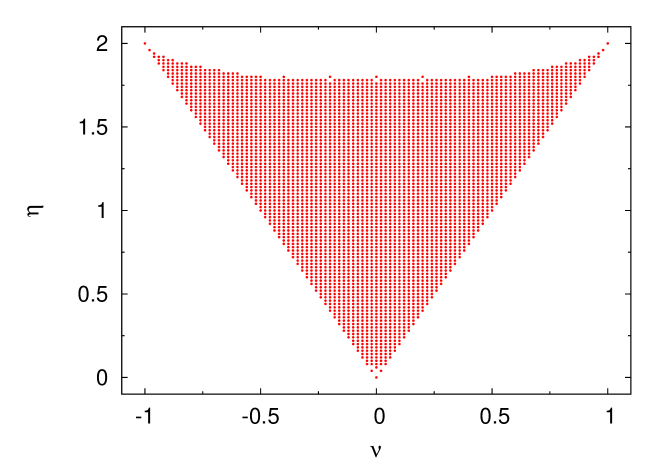
Figure 1 shows the CCs in the $n-m$ plane for the spin-1/2 Ising model with nearest-neighbor (NN) interactions, on a square lattice of $L\times L$ sites with periodic boundaries. [We use $n$ to denote the number of NN pairs of spins with the same orientation; the interaction energy of the antiferromagnetic (AF) Ising model is $E=-2(L^{2}-n)$.] Although the CCs tend to fill in a triangular region, some gaps are evident near the lower apex and along the upper edge. Knowing just which $(n,m)$ values are allowed for a given lattice size is important if we are to implement entropic sampling with confidence. In this paper we present a method for systematically enumerating all CCs of Ising models in the $(n,m)$ plane.

Figure 1: Allowed configuration classes for system size $L=10$; $\eta\equiv n/L^{2}$ and $\nu\equiv m/L^{2}$.

We study the spin-1/2 antiferromagnetic Ising model in an external magnetic field, whose energy is given by

$$\mathcal{H}=-J\sum_{<i,j>}\sigma_{i}\sigma_{j}-h\sum_{i=1}^{N}\sigma_{i}=-E-hm,$$ (1)

where $\sigma_{i}=\pm 1$, $<i,j>$ indicates a sum over NN pairs of spins, $h$ is the external field, and $N$ is the number of spins; the model is defined on a square lattice of $L\times L$ sites, with periodic boundary conditions. Unlike the ferromagnetic Ising model ($J>0$), which exhibits a unique critical point in the $h-T$ plane and has an exact solution [7], the AF model ($J<0$) possesses a critical line, which is not completely understood.

Various approximate methods have been applied to determine the critical line of the AF Ising model on the square lattice [8]^-[18]; these results, however, do not agree altogether. Binder and Landau [19] estimated the critical line via Monte Carlo simulation, obtaining very good agreement with the approximate closed-form expression of Müller-Hartmann and Zittartz [8], raising the possibility that the latter expression was in fact exact. (It was later shown that this is not so [12].) Hwang et al. [20] studied the AF Ising model on the square and triangular lattices using a microcanonical transfer matrix method and the Wang-Landau algorithm [3]. They performed an exact enumeration of the number of configurations, $\Omega(E,m)$, and found CSs in the $E-m$ plane similar to that shown in Fig. 1.

Using the tomographic entropic sampling (TES) algorithm [6] we estimate $\Omega(n,m,L)$, and associated microcanonical averages, for lattice sizes $L=10$ to 30, with an increment $\Delta L=2$. We then calculate the canonical averages of the thermodynamic quantities of interest. Using these data we map out the critical line in the $h-T$ plane, and compare our results with several theoretical expressions.

Prior determination of the set of allowed CCs is an important tool to verify the quality of the sampling: we want to be sure that all CCs are visited during the simulation. Since this algorithm uses an initial guess, $\Omega_{0}(n,m,L)$, to begin the study, it is convenient to use the final estimate $\Omega_{N}(n,m,L)$ (after the $N$-th iteration) to obtain the initial guess $\Omega_{0}(n,m,L_{0})$ of the next system size to be studied $(L_{0}>L)$. As we will show, good initial estimates, $\Omega_{0}(n,m,L)$, can be obtained using a two-dimensional interpolation because we know a priori the set of allowed CCs.

This paper is organized as follows. In Sec. 2 we define the basic CCs and the respective allowed values of $(n,m)$ for the spin-1/2 Ising model on the square lattice; the main goal of this section is to find all gaps in the $(n,m)$ plane. In Sec. 3, this information is used in simulations of the AF Ising model via the TES algorithm. There we describe the method used to determine $\Omega_{0}(n,m,L_{2})$ via two-dimensional interpolation of the final estimate, $\Omega_{N}(n,m,L_{1})$, of the previous system size studied. Simulation results are reported in Sec. 4, for the order parameter and the staggered susceptibility as functions of $h$ and $T$. Points along the critical line in the $h-T$ plane are obtained using finite size scaling analysis, and the results compared with several theoretical expressions. We summarize our findings in Sec. 5.

2 Configuration Classes

As pointed out above, one of the main problems in entropic sampling methods is the prior determination of the complete set of configuration classes for a given system size. Let us denote by $N_{+}$ and $N_{-}$ the number of up and down spins, respectively, on a square lattice with $N=N_{+}+N_{-}=L^{2}$ spins. The number of pairs of opposite spins, $u$, and $N_{+}$ are related to $n$ and $m$, respectively, via

$$n=2L^{2}-u$$ (2)

and

$$m=2N_{+}-L^{2}.$$ (3)

Thus, once the possible values of $(N_{+},u)$ are determined, so are those of $(n,m)$. Note that $u$, $n$ and $m$ can only take even values. The gaps in CS fall near the maximum and minimum values of $n$ ($n_{max}$ and $n_{min}$, respectively) for a given $m$. Therefore, we will identify the possible values of $u$ near its maximum, $u_{max}$, and minimum, $u_{min}$, for a given $N_{+}\in[0,\frac{L^{2}}{2}]$; note that the number of configurations is symmetric under interchange of $N_{+}$ and $N_{-}$.

2.1 Determining $u_{min}$ and nearby classes

2.1.1 Compact configurations

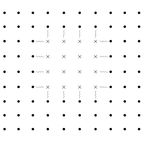
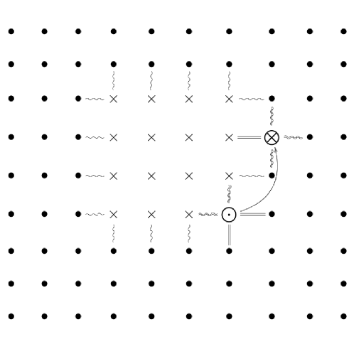
Compact configurations consist of a square or rectangular cluster with $N_{+}$ up spins. To begin, consider the case of a square cluster of size $l\times l$ $(2<l<L)$ with $N_{+}=l^{2}$, as is illustrated in Fig. 2. It is evident that this configuration corresponds to the minimum value of $u$, $u^{(0)}=4l$. A configuration with the same number of up spins, and $u=N_{+}+2$ is obtained by transferring an up spin from one of the corners of the square to an edge, as shown in Fig. 3. From this configuration, further rearrangements leading to $u=u_{min}+4$, etc., are possible. When $N_{+}$ is not a square number, the most compact configuration (i.e., with the smallest perimeter) is a rectangle, or a square or rectangle with an incomplete layer of sites along one edge. For $N_{+}=l(l-1)$ we have $u_{min}=4l-2$, while for $l(l-1)<N_{+}<l^{2}$, $u_{min}=4l$. In all cases, moving a corner site to an edge, one constructs a configuration with $u=u_{min}+2$, and further arrangements yield additional increases in $u$.

Figure 2: Basic compact configuration. Up and down spins are represented by “$\times$” and “$\bullet$”, respectively; wavy lines represent pairs of opposite spins.

Figure 3: Modified compact configuration. The new up and down spins are represented by “$\otimes$” (previously “$\bullet$”) and “$\odot$” (previously “$\times$”), respectively; double straight and double wavy lines represent new pairs of identical and opposite NNs, respectively.

2.1.2 Extended configurations

Thus there are no gaps in the large-$n$ region due to compact configurations. Such compact configurations, however, are not necessarily the ones that minimize $u$ for a given value of $N_{+}$. Consider for example the case $N_{+}=kL$ with $k$ an integer. The cluster of up spins can be arranged to wrap around the lattice, yielding $u_{min}=2L$, independent of $k$. We call such a configuration extended. For $k$ greater than a certain value, on the order of $L/4$, the configurations that minimize $u$ are extended rather than compact. Suppose now that for a given $N_{+}$, $u_{min}$ is obtained with an extended configuration, and that all compact configurations have $u$ strictly greater than $u_{min}$. If $N_{+}$ lies between $kL$ and $(k+1)L$, then the configuration that minimizes $u$ has at least two corners, and by the previous construction, configurations with $u=u_{min}+2$ exist. But if $N_{+}=kL$, the minimizing configuration has no corners and any modification yields a configuration with $u\geq u_{min}+4$. This is how the gaps near the maximum values of $n$ arise.

Summarizing, if $L$ and $N_{+}$ are such that $u_{min}$ is obtained with a compact configuration, then there are configurations with $u_{min}+2$, $u_{min}+4$, …, etc., and no gap exists. If, on the other hand, $u_{min}$ is realized only for an extended configuration, and $N_{+}$ is an integer multiple of $L$, then there are no configurations with $u=u_{min}+2$.

2.2 Determining $u_{max}$ and nearby classes

The largest possible value of $u$, $u_{max}$, occurs in a configuration such that $N_{+}=L^{2}/2$ with spins arranged in a chess board (CB) configuration, such that all up spins have down spins as NNs and vice versa. One readily verifies that for $0\leq N+\leq L^{2}/2$, the maximum number of unlike NN pairs is $u_{max}=4N_{+}$. Starting from the CB configuration, we can reduce $u$ by exchanging an up and a down spin. If the exchanged spins are NNs, the resulting configuration has $u=u_{max}-6$; otherwise one has $u=u_{max}-8$. Thus, for $N_{+}=L^{2}/2$, there are no configurations with $u=u_{max}-2$ or $u_{max}-4$. One readily verifies that configurations with $u=u_{max}-10$, $u_{max}-12$, etc., can be obtained via further exchanges of spins.

For $N_{+}=L^{2}/2-1$, we have $u_{max}=2L^{2}-4$. Such configurations can be constructed by flipping one up spin in the CB configuration. Starting from this configuration, exchanging a pair of spins, one can reduce $u$ by 4, 6 or 8, but there is no rearrangement which reduces $u$ by just two. Thus for $N_{+}=L^{2}/2-1$, there is no configuration having $u=u_{max}-2$; configurations with $u=u_{max}-4$, $u_{max}-6$, etc. do exist.

Finally, we note that for $1<N+<L^{2}/2-1$, there are no gaps in the neighborhood of $u_{max}$. To verify this, consider a configuration obtained by flipping $k$ up spins in the CB configuration, so that $N_{+}=L^{2}/2-k$, where $1<k<L^{2}/2$. By hypothesis there are now at least four more sites with down spins than with up spins. Starting from a configuration with $u=u_{max}$, in which each up spin is surrounded by down spins, we can create a single NN pair of up spins, with all six neighbors down, and with all remaining up spins completely surrounded by down spins. In this manner, $u$ is reduced by two. Configurations with $u=u_{min}-4$, $u_{min}-6$, etc. can be obtained by further exchanges of up and down spins.

Using the facts summarized above, it is straightforward to construct an algorithm that determines which values of $u$ are possible, for a given $L$ and $N_{+}$, and thereby which values $(n,m)$ are accessible for a given system size. In the simulations reported below, we have verified that our entropic sampling scheme converges to visit all allowed classes.

3 Implementation

Using tomographic sampling, we study the antiferromagnetic Ising model in an external field on the square lattice; we consider periodic boundary conditions and NN interactions. The CCs of the systems are defined in the energy-magnetization space $(n,m)$.

The TES method is applied in order to generate estimates of $\Omega(n,m,L)$. For the smallest system size $(L=10)$ we begin with a guess, $\Omega_{0}(n,m)$, obtained using a mean-field approximation. For subsequent system sizes, however, we use a two-dimensional interpolation of $\Omega_{N}(n,m,L)$ (the final estimate of $(n,m)$ for the smaller system size, $L$) to construct $\Omega_{0}(n,m,L^{\prime})$, where $L^{\prime}>L$. For most studies we use five iterations, each one with $N_{sim}=10$ initial configurations, which are simulated for $N_{U}=10^{7}$ lattice updates or Monte Carlo steps.

Let us denote by $\Gamma(n,m)$ and $\Gamma^{\prime}(n_{0}=n+\Delta n,m_{0}=m+\Delta m)$ the CCs that contain configurations $\mathcal{C}$ and $\mathcal{C^{\prime}}$, respectively. The simulation uses a single spin-flip dynamics, so that the possible variations of $n$ and $m$ are $\Delta n=0,\pm 2,\pm 4$ and $\Delta m=\pm 2$. At iteration $j$, the acceptance probability for the transition $(\mathcal{C}\to\mathcal{C^{\prime}})$ is

$$p_{j}(\Gamma\to\Gamma^{\prime})=\textrm{min}\bigg{[}\frac{\Omega_{j-1}(\Gamma)}{\Omega_{j-1}(\Gamma^{\prime})},1\bigg{]}.$$ (4)

These probabilities are stored in a table. For each configuration generated, be it a new one (if it is accepted) or the same (if it is rejected), we update the sums used to calculate the microcanonical and canonical averages of $\phi$, $|\phi|$, $\phi^{2}$, and $\phi^{4}$, where

$$\phi\equiv m_{A}-m_{B}$$ (5)

is the order parameter (staggered magnetization); $m_{A,B}$ are the magnetizations of the two sublattices. At the end of each iteration $j$ the estimate of $\Omega_{j}(n,m)$ is refined according to

$$\Omega_{j}(\Gamma)=\frac{H_{j}(\Gamma)}{\overline{H}_{j}(\Gamma)}\,\Omega_{j-1}(\Gamma),$$ (6)

where $H_{j}(\Gamma)$ is the histogram containing the number of times the CC $\Gamma$ is visited during the sampling, and $\overline{H}_{j}(\Gamma)$ is the average of $H_{j}(\Gamma)$ over all accessible CCs; the acceptance probability [Eq. (4)] is updated using the new estimate of $\Omega_{j}(n,m)$ and the histogram, $H_{j}(n,m)$, is set to zero.

A single iteration of our method consists of ten independent simulations, each involving $10^{7}$ lattice updates, and each beginning from a different initial configuration. (By a lattice update we mean one attempted flip per spin; the initial configurations include, high, low, and intermediate interaction energies and both signs of the magnetization.)

3.1 Determining $\Omega_{0}(n,m,L)$: mean field approach

As noted above, for the smallest system size we use an estimate of $\Omega_{0}(n,m,L)$ obtained via a mean-field approximation, specifically

$$\frac{1}{L^{2}}\ln\Omega_{0}(n,m,L)=\frac{1}{L^{2}}\ln\Omega(m)-\frac{(n-\langle n\rangle)^{2}}{2L^{2}\sigma^{2}}-\frac{\ln\sigma}{L^{2}}+const.\,,$$ (7)

where $\sigma\equiv\sigma(m)=\sqrt{\textrm{var}(n)}$, and

$$\frac{\ln\Omega(m)}{L^{2}}\simeq\ln 2-\frac{1}{2}[(1+m/L^{2})\ln(1+m/L^{2})+(1-m/L^{2})\ln(1-m/L^{2})].$$ (8)

To obtain this expression, we first note that $\Omega(m,L)=\sum_{n}\Omega(n,m,L)=\binom{L}{N_{+}}$, and use Stirling’s approximation. The dependence on $n$ is then obtained by estimating $\langle n\rangle$ and $\textrm{var}(n)$ for a given $m$ and $L$, using a random-mixing approximation, and supposing that $n$ follows a Gaussian distribution.

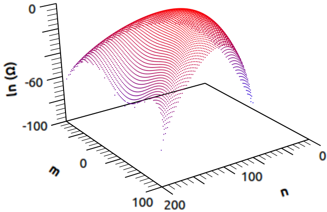
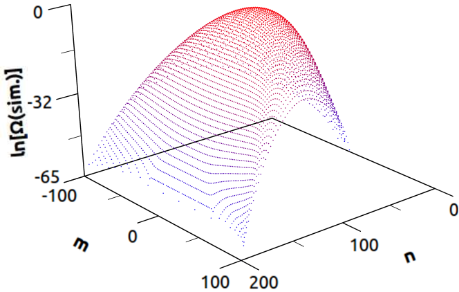
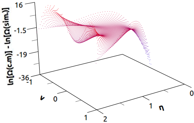
In Fig. 4 we plot the estimate of $\ln\Omega_{0}(n,m,L=10)$ given by Eq. (7). We present in Fig. 5 the final estimated value of $\ln\Omega_{5}(n,m,L=10)$ after the 5$th$ iteration of the simulation; this result is quite similar to that presented by Hwang et al. [20] for the square lattice, which was obtained using Wang-Landau sampling [3]. We note that the differences between the initial estimate obtained via mean field approximation and the final simulation result of $\ln\Omega(n,m,L=10)$ are more evident near the edges of the CS, specially near to the maximum values of $n$. To have a better idea of how close this initial estimate is to the final simulation result, we plot in Fig. 6 the difference between that estimate and the final result of the simulation for $L=10$. Analyzing this figure, it is again clear that the differences are larger near the edges of the CS.

Figure 4: Estimate of $\ln\Omega_{0}(n,m,L=10)$ via mean-field approximation.

Figure 5: Final estimate of $\ln\Omega_{5}(n,m,L=10)$ after the 5$th$ iteration of the simulation.

Figure 6: Difference between $\ln\Omega_{0}(n,m,L=10)$, estimated via mean-field approximation, and the final simulation result after the 5th iteration, $\ln\Omega_{5}(n,m,L=10)$.

3.2 Determining $\Omega_{0}(n,m,L)$: interpolation

We expect that the closer the estimate $\Omega_{0}(n,m)$ is to the (unknown) exact value, $\Omega_{e}(n,m)$, the faster the simulation will converge, and the more accurate our final estimate will be. Since the mean-field estimate worsens as the system size grows, we only use it for the smallest system size studied; initial estimates of subsequent system sizes are obtained by interpolating the final estimate, $\Omega_{N}(n,m,L)$, of the previous system size studied. Our procedure is based on the existence of the limiting microcanonical entropy density as a function of the intensive parameters $\eta$ and $\nu$ (the bond and magnetization densities, respectively),

$$s(\eta,\nu)=\lim_{L\to\infty}\frac{1}{L^{2}}\ln\Omega(n_{L},m_{L},L),$$ (9)

where $n_{L}\simeq\eta L^{2}$ and $m_{L}\simeq\nu L^{2}$. (Since $n$ and $m$ are restricted to even integers we have $n_{L}=\eta L^{2}+{\cal O}(1/L^{2})$ and similarly for $m_{L}$.) The idea is then to write

$$\frac{1}{L^{\prime 2}}\ln\Omega_{0}(n^{\prime},m^{\prime},L^{\prime})=\frac{1}{L^{2}}\ln\Omega_{N}(\eta L^{2},\nu L^{2},L),$$ (10)

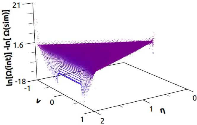
where $\eta=n^{\prime}/L^{\prime 2}$, $\nu=m^{\prime}/L^{\prime 2}$, and the r.h.s. is evaluated by extending $\ln\Omega_{N}$ to noninteger $n$ and $m$ via extrapolation and interpolation. Using this approach, we obtain better estimates, as is shown in Fig. 7. (Note that the largest differences continue to fall along the edges of the CS.)

Figure 7: Difference between $\ln\Omega_{0}(n,m,L=18)$, estimated by interpolating the final result of $L=16$, and the final simulation result after the 5th iteration, $\ln\Omega_{5}(n,m,L=18)$.

3.3 Extrapolation and interpolation

Suppose we wish to construct the initial estimate $\Omega_{0}(n,m,L_{2})$ on the basis of the simulation results for a smaller system, $\Omega_{N}(n,m,L_{1})$. We could do this via interpolation if every CC of the larger system were surrounded by four points of the smaller one in the $\eta$-$\mu$ plane. Fig. 8 shows, however, that along the edges of the CS, the points corresponding to classes of the larger system are not surrounded by four points of the smaller one. For those points, one could in principle use extrapolation rather than interpolation. We found, however, that direct extrapolation yields poor estimates for $\Omega$.

Figure 8: Region of the $(\eta,\nu)$ plane with every possible configuration classes for system sizes $L_{1}=26$ and $L_{2}=28$.

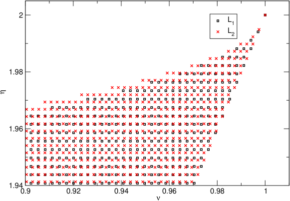
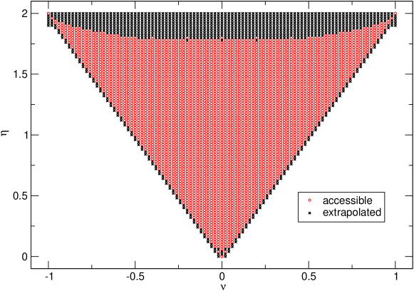
We obtain better estimates by first extrapolating the points along the edges of the CS for the smaller system, such that every point of the larger system is surrounded by four points of the smaller. Figure 9 shows the CS with accessible and extrapolated CCs for $L=10$. Following this extrapolation we perform a linear two-dimensional interpolation as per Eq. (10).

Figure 9: Accessible and extrapolated configuration classes of a system of size $L=10$.

4 Results

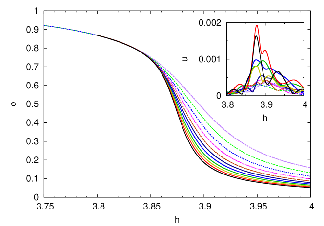
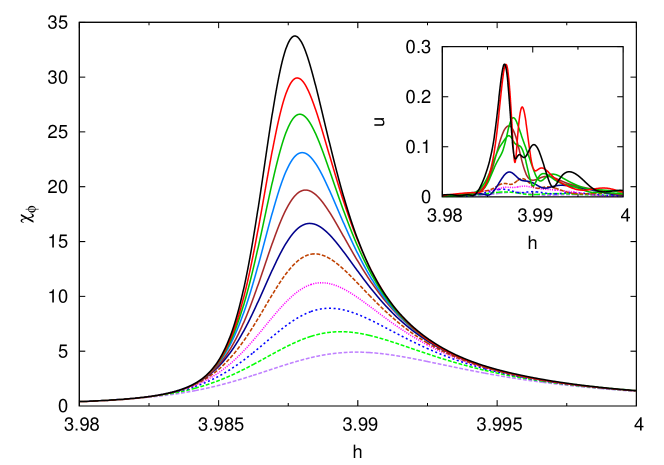
In this section we present results of the AF Ising model on the square lattice in an external field; periodic boundary conditions are employed. We use TES to simulate systems of sizes $L=10$ to 30, with $\Delta L=2$. To calculate the uncertainties we perform five independent studies for each system size. We plot in Fig. 10 the staggered magnetization (order parameter) per site, $\phi$, as a function of $h$ at $T=0.2$. We can see that $\phi$ decreases considerably between $h=3.85$ and $h=3.90$; this behavior suggests a critical point, $h_{c}$, marking a phase transition from the AF to the paramagnetic state. Figure 11 shows the staggered susceptibility per site,

$$\chi_{\phi}\equiv\frac{1}{L^{2}}(\langle\phi^{2}\rangle-\langle\phi\rangle^{2}),$$ (11)

as a function of $h$ at $T=0.02$. As $L$ grows the peaks tend to the critical point, $h_{c}$. The specific heat per site, $c$, (not shown) has a similar behavior.

Figure 10: Staggered magnetization per site as a function of $h$ at $T=0.2$, for $L=10$ to 30. The absolute uncertainties are plotted in the inset.

Figure 11: Staggered susceptibility per site as a function of $h$ at $T=0.02$, for $L=10$ to 30. The highest peaks correspond to the largest system sizes. The absolute uncertainties are plotted in the inset.

4.1 Phase diagram

Using finite size scaling analysis [21] we estimate the critical line, $h_{c}(T)$, or, equivalently, $T_{c}(h)$, via the relations:

$$h_{c}(Y_{max},T,L)=h_{c}(Y_{max},T)+a_{1}/L+a_{2}/L^{2},$$ (12)

and

$$T_{c}(Y_{max},h,L)=T_{c}(Y_{max},h)+b_{1}/L+b_{2}/L^{2},$$ (13)

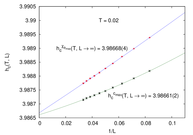
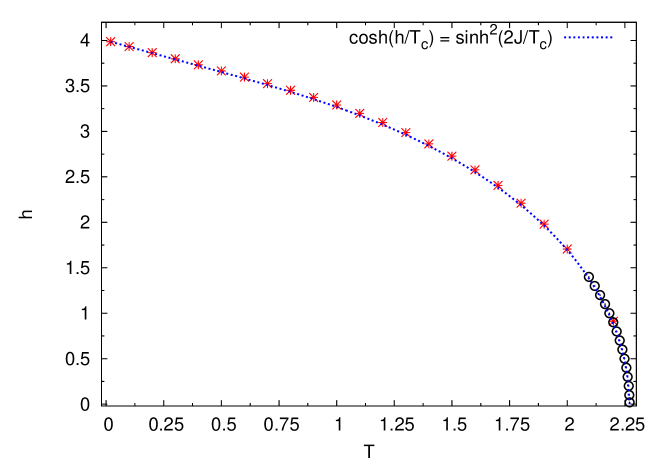
where $h_{c}(Y_{max},T,L)$ is the field at which $Y$ (the specific heat or the staggered susceptibility) takes its maximum for a given temperature and system size; $T_{c}(Y_{max},h,L)$ is defined in an analogous manner. The estimates obtained using the maximum of $c$ and $\phi$ are averaged to yield $h_{c}(T)$ and $T_{c}(h)$; Figure 12 illustrates the procedure for estimating $h_{c}$, for $T=0.02$. Our estimated points for the phase boundary are shown in Fig. 13 along with the approximate expression derived by Müller-Hartmann and Zittartz [8]:

$$\cosh\bigg{(}\frac{h}{T_{c}}\bigg{)}=\sinh^{2}\bigg{(}\frac{2J}{T_{c}}\bigg{)}.$$ (14)

Our simulation results are in good agreement with their expression. For the critical field, the greatest relative difference between theory and simulation is about 0.9%, which occurs at $T_{c}=1.8$.

Figure 12: Critical field determination using finite size scaling analysis: $\overline{h}_{c}(T=0.02)=3.98666(3)$.

Figure 13: Phase diagram of the Ising AF on the square lattice. Comparison between simulation and the theoretical expression of Müller-Hartmann and Zittartz. Asterisks denote points obtained varying $h$ with $T$ fixed; circles denote points obtained varying $T$, with $h$ fixed. The error bars of our results are smaller than the symbols.

In Table 1 we compare our simulation estimates for the critical magnetic field $h_{c}(T)$ with some theoretical approximations. For temperature $T\leq 1$ we find good agreement with the estimates of Monroe [17] (whose analysis involves a free parameter $\omega$), Wu and Wu [12], and Blöte and Wu [13], whereas there are significant discrepancies in relation to the other approximations. At higher temperatures, differences appear between simulation and the predictions of Monroe, Wu and Wu, and Blöte and Wu. These may reflect a small systematic error or an underestimate of simulation uncertainties. We intend to examine this issue in greater detail in future work.

Table 1: Comparison between our simulation estimates of $h_{c}(T)$ with some theoretical approximations.

$T$	TES	Monroe	Monroe	MHZ	WW	BW	WK
		$(\omega=0.92484)$	$(\omega=0.93895)$
0.1	3.93304(16)	3.93307	3.93318	3.93069	3.93329	3.93330	3.93372
0.5	3.6648(8)	3.66506	3.66561	3.65309	3.66611	3.66614	3.67589
1.0	3.2906(14)	3.29303	3.29391	3.26843	3.29200	3.29261	3.31764
1.5	2.7258(14)	2.73243	2.73396	2.70401	2.73094	2.73176	2.75099
2.0	1.696(2)	1.71629	1.71872	1.69490	1.71492	1.71499	1.71512
TES: Tomographic entropic sampling [6]
MHZ: Müller-Hartmann and Zittartz [8]
WW: Wu and Wu [12]
BW: Blöte and Wu [13]
WK: Wang and Kim [16]

5 Conclusions

The complete enumeration of CCs is of fundamental importance to study the antiferromagnetic Ising model using tomographic entropic sampling. The determination of CCs for entropic sampling of Ising models also enables us to obtain good initial estimates for the configuration numbers $\Omega_{0}(n,m,L)$, using two-dimensional linear interpolation; the initial estimate is reasonably close to the final estimate $\Omega_{N}$. Despite the relatively small system sizes used in this study, we obtain a good estimate for the critical line in the temperature-magnetic field plane. Further details on critical behavior will be published elsewhere [22].

References

- [1] B. A. Berg and T. Neuhaus, Phys. Rev. Lett. 68, 9 (1992).
- [2] J. Lee, Phys. Rev. Lett. 71, 211 (1993).
- [3] F. Wang and D.P. Landau, Phys. Rev. Lett., 84, 10 (2001).
- [4] F. Wang and D.P. Landau, Phys. Rev. E, 63, 056101 (2001).
- [5] M.E.J Newman and G.T. Barkema. Monte Carlo Methods in Statistical Physics (Oxford University Press, New York, 2001), p. 161 - 169.
- [6] R. Dickman and A.G. Cunha-Netto, Phis. Rev. E, 84, 026701 (2011).
- [7] L. Onsager, Phys. Rev., 65, 117 (1944).
- [8] E. Müller-Hartmann and J. Zittartz, Z. Phys., 73, 261 (1977).
- [9] L. Sneddon, J. Phys. C, 12, 3051 (1979).
- [10] R.R. Santos, J. Phys. C, 18, L1067 (1985).
- [11] M. Kaufman, Phys. Rev. B, 36, 3697 (1987).
- [12] X.N. Wu and F.Y. Wu, Phys. Lett. A, 144, 123 (1990).
- [13] H.W.J. Blöte and X-N. Wu, J. Phys. A, 23, L627 (1990).
- [14] M. Badehdah, A. Benyoussef and M. Touzani, J. Magn. Magn. Mater., 172, 254 (1997).
- [15] X-Z. Wang and J.S. Kim, Phys. Rev. Lett., 78, 413 (1997).
- [16] X-Z. Wang and J.S. Kim, Phys. Rev. E, 56, 2793 (1997).
- [17] J.L. Monroe, Phys. Rev. E, 64, 016126 (2003).
- [18] S.J. Penney, V.K. Cumyn and D.D. Betts, Physica A, 330, 507 (2003).
- [19] K. Binder and D.P. Landau, Phys. Rev. B, 21, 5 (1980).
- [20] C-O. Hwang, S-Y. Kim, D. Kang and J.M Kim, J. Stat. Mech: Theory Exp., 2007, L05001 (2007).
- [21] V. Privman. Finite Size Scaling Analysis and Numerical Simulations of Statistical Systems (World Scientific, London, 1990).
- [22] B.J. Lourenço and R. Dickman, in preparation.