Customer Equilibrium and Optimal Strategies
in an $M/M/1$ Queue with Dynamic Service Control

Abstract

We consider the problem of customer equilibrium strategies in an M/M/1 queue under dynamic service control. The service rate switches between a low and a high value depending on system congestion. Arriving customers do not observe the system state at the moment of arrival. We show that due to service rate variation, the customer equilibrium strategy is not generally unique, and derive an upper bound on the number of possible equilibria. For the problem of social welfare optimization, we numerically analyze the relationship between the optimal arrival rate, which maximizes the overall welfare of the customers, and the equilibrium ones as a function of various parameter values. We finally derive analytic solutions for the special case where the service rate switch occurs when the queue ceases to be empty.
Keywords: Queueing; Customer Equilibrium Strategies; Dynamic Service Control; Positive Externalities; Social Welfare Maximization.

1 Introduction

Service rate control is a prevalent tool for dynamically adjusting the operation of a queueing system in response to varying congestion levels. Many models in the queueing and service management literature, such as dynamic staffing policies, server vacation mechanisms, etc. can be viewed as different aspects of varying the rate at which service is provided at different times. In most cases, the philosophy of a service control policy is to increase the service capacity when the congestion level is high in order to alleviate excessive delays, and reduce it at times of decreased congestion in order to lower operating costs. Viewed in this way, a service control policy provides a balance in the tradeoff between long customer delays and high service costs. However, in situations where customers are sensitive to delay and make individual decisions about entering the queue, the policy used by the service provider may also have an indirect, albeit significant, effect on the arrival stream.

In service systems with strategic customer behavior, incoming customers decide independently whether to join the system or balk, based on an individual utility function that combines the value of obtaining the service with the cost induced by the anticipated delay in the queue. Since a customer’s delay depends on the decisions of other customers, a game-theoretic approach is appropriate for characterizing customer behavior and thus the properties of the incoming stream, as the result of an equilibrium strategy. Because customers are averse to delay, it is expected that a particular customer’s decision to enter the system is adversely affected as other customers also decide to enter and system congestion is increased. In economic terms, entering customers induce negative externalities, by imposing increased delays to present and/or future arrivals. Such situations, where in equilibrium a customer’s willingness to join is a decreasing function of the arrival rate, are referred to as Avoid the Crowd (ATC). On the other hand, in a system where a form of dynamic service control is implemented, the service rate is usually increased when the system is congested. Thus, it may happen that if a customer decides to enter the system, the other customers experience a benefit, because the service provider is induced to increase the service rate. Then, the net effect between the additional delay due to increased arrivals and the higher service speed due to the server’s policy may be positive. In such cases where an arriving customer induces positive externalities, the equilibrium is Follow the Crowd (FTC). Both the ATC or FTC effects may appear in the same system for different values of the arrival rate. However in most situations, the presence of FTC is related to a dynamic service policy employed by the service provider.

In this paper we analyze the customer equilibrium behavior in a single server Markovian queue under a simple threshold-based service rate policy. Specifically, the service rate is kept at a low value when the number of customers in the system is at or below a threshold level $T$, and turns to a high value when the system congestion is above $T$. We analyze the unobservable case where arriving customers are aware of the service policy, but do not have any information on the queue length upon arrival. The most pronounced effect of the service control policy is that, in contrast to the simple M/M/1 queue in strategic equilibrium, the equilibrium customer strategy is not generally unique. For example, one equilibrium strategy may be such that a small fraction of incoming customers joins the system and as a result the server works at slow rate for most of the time, whereas there exists another equilibrium where the arrival rate is high and the server spends most time at the fast mode. We show that, depending on the values of the various parameters, the number of strategic equilibria may vary from one to at most three. We also consider the problem of determining the optimal arrival rate in a system with centrally control arrivals which, for the given service policy, maximizes the expected net benefit of all customers, and compare the optimal arrival rates to those obtained as equilibria under selfish customer behavior.

The implications of strategic customer behavior on the performance of a queueing system has been studied extensively in the recent years. Early works on the M/M/1 queue include Naor (1969) and Edelson & Hildebrand (1975) for the observable and unobservable models, respectively. Many variations of the original models have been studied since, and a comprehensive review of the literature until 2003 is provided in Hassin & Haviv (2003). Among the models that have been developed and analyzed, many include some varying service rate characteristics indirectly. For example, the capacity choice problem can be viewed as long-term service rate decision. Stenbacka & Tombak (1995) consider an unobservable system with nonhomogeneous customer delay costs and service rate decisions made by the firm. Chen & Frank (2004) analyze the joint impact of a firm’s service and pricing policy on customer equilibrium.

In observable models, where customers obtain full or partial information on system congestion or anticipated delay, a varying service rate policy may have analogous effects. Armony & Maglaras (2004) analyze the impact of announcing anticipated delays and providing a call back option on customer joining behavior, in a call center with two service modes. Debo & Veeraraghavan (2009) consider a situation where the service rate is related to the quality of service, it is unknown to arriving customers but can be estimated by observing the queue length. It is shown that when the service rate and the quality of service are negatively correlated, customers join longer queues, which is not the case under positive correlation.

Other systems with a varying service rate feature include vacation queues and systems in a random environment. Burnetas & Economou (2007) consider a system with server vacations and reactivation that requires a random setup time. In the vacation model of Guo & Hassin (2011), the server resumes service after a fixed number of arrivals according to a threshold service policy. Both papers analyze equilibrium behavior with respect to several levels of information about the queue length and the state of the server. Economou & Manou (2011) analyze customer equilibrium strategies in a stochastic clearing system where the exogenous customer arrival rate and the arrival rate of the system clearing server vary according to an external environment process.

In the area of queueing control and optimization under a single decision maker, problems of service rate control have been studied extensively and in many forms. It is worth noting that the problem of social welfare maximization can be formulated as a static or dynamic admission control problem. George & Harrison (2001) consider welfare optimization in an $M/M/1$ system with dynamic service control and constant arrival rate. They develop an asymptotic method for computing the optimal policy under average cost minimization. Ata & Shneorson (2006) propose a model that jointly optimizes arrival and service rates, and develop a dynamic pricing strategy that induces the optimal arrival and service rates. Adusumilli & Hasenbein (2010) consider a model of joint admission and service control in an $M/M/1$ under an average cost criterion and show that the optimal service rates are increasing with system congestion. Dimitrakopoulos & Burnetas (2011) analyze the effect of service rate flexibility on the admission control policy and the service provider’s profit and derive a condition for the service flexibility to be beneficial.

The present paper proposes a direct model of the impact of dynamic service control on customer equilibrium strategies. The service rate is dynamically adjusted with state congestion. Under this situation, the delay function is not monotone increasing in the arrival rate, which implies that for certain ranges of the arrival rate, joining customers impose positive externalities. Another consequence is that in general there exist more than one strategic equilibria, however we show that their number is at most three. We also consider the social welfare optimization problem and the relationship between the equilibrium and optimal arrival rates. We show via computational experiments that optimal arrival rate lies between the extreme values under equilibrium, due to the existence of both negative and positive externalities.

The rest of the paper is organized as follows. In Section 2 we introduce the model and the corresponding customer strategic behavior problem. We also derive the expected delay as a function of the arrival rate. In Section 3 we consider the equilibrium strategies and derive the upper bound on the number of equilibria for general $T$-threshold dynamic service policies. In Section 4 we explore numerically the socially optimal strategy and the comparison with the equilibrium problem. In Section 5, we derive analytic solutions for both problems in the special case where the service threshold $T=1$, i.e., the service rate switches to the fast mode when the queue is not empty. Section 6 concludes.

2 Model Description

We consider a single server Markovian queue under the FCFS discipline, where potential customers arrive according to a Poisson process with rate $\Lambda$. The service rate is dynamically set according to a $T$-threshold policy. Specifically, the service rate is set to $\mu_{l}$ whenever the number of customers in the system is less than or equal to $T$, and equal to $\mu_{h}$ otherwise, where $\mu_{l}<\mu_{h}$. There are no switching costs. Thus, the service policy is defined by the parameters $(T,\mu_{l},\mu_{h})$, which are known to all arriving customers.

Arriving customers are assumed identical. They make the decision whether to join or balk upon arrival, in order to maximize their expected net benefit, thus they are assumed risk neutral. Every joining customer receives a fixed reward $R\geq 0$ upon service completion, and incurs a service cost rate $C>0$ per time unit of delay. In addition, each arriving customer has no information for the queue length prior to entering the system.

Since the join decisions of individual customers affect the system delay and thus the benefit of all customers, the decision problem corresponds to a symmetric game. We restrict attention to symmetric Nash equilibrium strategies defined as follows.

Given that potential customers are not aware of the actual system state, an arriving customer has two pure strategies, either to join the system or balk. However, for the equilibrium analysis, mixed strategies also have to be considered. A mixed strategy is defined by $p\in[0,1]$, the probability of joining the system, where for $p=0,\;\hbox{or}\;1$ it reduces to a pure strategy.

Let $U(p;q)$ denote a tagged customer’s expected net benefit from using mixed strategy $p$, when all others adopt mixed strategy $q$. Then, a mixed strategy $q^{e}$ is a symmetric Nash equilibrium strategy, if $U(q^{e},q^{e})\geq U(q,q^{e})$ for any mixed strategy $q\in[0,1]$. The intuition is that an equilibrium strategy is the best response against itself, so if all customers agree to follow mixed strategy $q^{e}$, no one can benefit from changing it.

Under a mixed strategy $q$ arrivals follow a Poisson process with effective arrival rate $\lambda=\Lambda q$. The corresponding equilibrium arrival rate is denoted by $\lambda^{e}=\Lambda\cdot q^{e}$, where $q^{e}$ is a symmetric equilibrium strategy. In addition, the customer’s expected net benefit is equal to

$$U(p;q)=p\left[R-CW(\Lambda q)\right],$$ (1)

where $W(\lambda)$ denotes the total sojourn time of a customer in the system, as a function of the effective arrival rate $\lambda$, assuming $\lambda<\mu_{h}$, in order to ensure stability.

In the remainder of the paper, we refer to $W(\lambda)$ as the waiting time or the delay function and, without loss of generality, we normalize $\mu_{h}=1$ and $C=1$.

An alternative decision framework could be defined by assuming that all customer decisions are controlled by a central planner, who enforces a mixed strategy $q$ with the objective of maximizing the overall expected net benefit per unit time. This corresponds to the social welfare optimization problem.

Given that a common strategy $q$ corresponds to a Poisson arrival rate $\lambda=\Lambda q$, the welfare function can be defined in terms of $\lambda$ as

$$S(\lambda)=\lambda\left[R-W(\lambda)\right]\;\hbox{for}\;\lambda\in[0,1)$$ (2)

and an arrival rate $\lambda^{*}$ is socially optimal if

$$S(\lambda^{*})=\max_{\lambda\in[0,1)}S(\lambda).$$ (3)

In general the equilibrium and optimal arrival rates rates do not coincide.

In the following sections we analyze the equilibrium and social optimization problems and their relationship.

In the remainder of this section we derive the expression for the delay function $W(\lambda)$.

An unobservable $M|M|1$ queue under a T-threshold service policy and a common mixed strategy $q$ for all customers corresponds to a standard birth and death process with arrival rates $\lambda_{n}=\lambda=\Lambda q,\;n\in{\bf{N}}$ and departure rates $\mu_{n}=\left\{\begin{array}[]{ll}\mu_{l},&n\leq T\\ 1,&n>T\end{array}\right.,\;n\in{\bf{N^{*}}},$ where $n$ refers to the number of customers in the system.

Using standard queueing analysis, we derive the following expression for the waiting time

$$W(\lambda)=\frac{\frac{1}{\mu_{l}-\lambda}\{\mu_{l}^{T}-(T+1)\lambda^{T}+\frac{\lambda}{\mu_{l}-\lambda}(\mu_{l}^{T}-\lambda^{T})\}+\frac{\lambda^{T}(T+1-T\lambda)}{(1-\lambda)^{2}}}{\frac{\mu_{l}^{T+1}-\lambda^{T+1}}{\mu_{l}-\lambda}+\frac{\lambda^{T+1}}{1-\lambda}},$$ (4)

for $\lambda\in[0,\mu_{l})\cup(\mu_{l},1)$.

An analogous expression of $W(\lambda)$ can be obtained for the case $\lambda=\mu_{l}$. After simplification both expressions can be reduced to the following, in which the denominator is strictly positive in $\lambda\in[0,1)$:

$$W(\lambda)=\frac{(\mu_{l}-\lambda)^{2}g(\lambda)}{(1-\lambda)(\mu_{l}-\lambda)^{2}d(\lambda)}=\frac{g(\lambda)}{(1-\lambda)d(\lambda)},\;\hbox{for any}\;\lambda\in[0,1),$$ (5)

where

$$g(\lambda) = -(T-1)(1-\mu_{l})\lambda^{T}$$ (6)

$$-(1-\mu_{l})\sum_{j=1}^{T-1}\mu^{j-1}_{l}\left[(T-(j+1))\mu_{l}+j-1-T\right]\lambda^{T-j}+\mu^{T-1}_{l}$$

and

$$d(\lambda)=(1-\mu_{l})\sum_{j=0}^{T-1}\mu^{j}_{l}\lambda^{T-j}+\mu^{T}_{l}.$$ (7)

Note that, $W(0)=\frac{1}{\mu_{l}}>0$ and $\lim_{\lambda\rightarrow 1^{-}}W(\lambda)=+\infty$.

In addition, using (5) we obtain a lower bound for the waiting time:

$$W(\lambda)>\frac{1}{1-\lambda},$$ (8)

where the right-hand side is the expected waiting time in an $M|M|1$ queue with service rate equal to $1$.

3 Equilibrium Analysis

In this section, we identify the equilibrium strategies under individual customer behavior.

Using the standard methodology of equilibrium analysis in

unobservable queueing models (see Hassin & Haviv (2003) p. 46-47), we derive from (1) the following equilibria:

$$\lambda^{e}=0\;\hbox{if and only if}\;W(0)=\frac{1}{\mu_{l}}\geq R.$$ (9)

Note that, when $R<1$, $0$ is the unique symmetric equilibrium, because of (8). Similarly,

$$\lambda^{e}=\Lambda\;\hbox{if and only if}\;W(\Lambda)<R.$$ (10)

In addition, a necessary and sufficient condition, for $\lambda^{e}=\Lambda q^{e}\in(0,1)$ to be an equilibrium arrival rate is that

$$U(q^{e};\lambda^{e})=0,\;\hbox{or equivalently,}\;W(\lambda^{e})=R.$$ (11)

Thus, the problem of identifying symmetric equilibria other than the extreme $\lambda^{e}=0$ or $\Lambda$, is equivalent to finding the solutions of the equation

$$W(\lambda)=R,\;\hbox{in}\;\lambda\in(0,1),\;\hbox{for}\;R\geq 1.$$ (12)

In the following we assume without loss of generality that the external arrival rate $\Lambda\geq 1$, in order to identify all possible equilibrium arrival rates $\lambda^{e}$ in the interval $[0,1)$. In the case where $\Lambda<1$, some of these equilibria may be excluded and instead we must also consider $\Lambda$ as a possible equilibrium arrival rate.

From the properties of the delay function $W(\lambda)$ we derive the following lemma.

Lemma 1

If $R>\frac{1}{\mu_{l}}$, then the equation $W(\lambda)=R$ has at least one solution in $\lambda\in(0,1)$.

Proof   From the divergence of $W(\lambda)$ to infinity as $\lambda\rightarrow 1^{-}$, we derive that for any $R\geq 1$, there exists an arrival rate $\lambda_{0}\in(0,1)$ such that $W(\lambda_{0})\geq R$.

In addition, $W(0)=\frac{1}{\mu_{l}}<R$ and the result follows readily from the continuity of $W(\lambda)$ in $\lambda\in[0,\lambda_{0}]$.   

Figure 1: The expected waiting time, $W(\lambda)$, for (a)$T=3,\;\mu_{l}=\frac{1}{10}$ and (b)$T=10,\;\mu_{l}=\frac{1}{5}$

From Lemma 1, it follows that for $R>\frac{1}{\mu_{l}}$ there exists at least one positive equilibrium arrival rate. On the other hand, extensive numerical analysis for different values of the parameters $R,\;T$ and $\mu_{l}$ has shown that there are at most three symmetric equilibria $\lambda^{e}\in(0,1)$.

This observation is consistent with the behavior of the delay function $W(\lambda)$, as demonstrated in Figure 1 for two typical cases of $T$-threshold policies $(T,\mu_{l},1)$. In both plots, we observe that $W(\lambda)$ increases for low and high values of $\lambda$, whereas for intermediate values of $\lambda$, it decreases. Intuitively, this is happening because for small and large values of $\lambda$, the system spends almost all time in the low or high service rate state, respectively, and the delay is approximately that of an $M|M|1$ queue with the corresponding value of $\mu$.

On the other hand, for intermediate values of $\lambda$, the service rate switch occurs more often. In this case, increasing $\lambda$ increases the rate of arrival to the queue, but at the same time forces the server to work faster and the net effect may be a decrease in the overall delay.

Because of the non-monotone behavior of $W(\lambda)$, the number of roots of (12) may vary from $0$ to $3$, depending on the values of $R,\;T$ and $\mu_{l}$.

For example in Figure 1(a), for $R=9$, there are three equilibrium arrival rates, one of which equal to zero, while in Figure 1(b) for $R=21$, there are three strictly positive equilibria.

Note that this discussion is solely based on observation of the delay function graph for different numerical values. The complexity of the expressions does not allow the study of $W(\lambda)$ directly.

We instead resort to the following equivalent polynomial equation of degree $T+1$, derived by substituting (5) in (12).

$$H(\lambda) = -R(1-\mu_{l})\lambda^{T+1}+(1-\mu_{l})(R(1-\mu_{l})+T-1)\lambda^{T}$$

$$+(1-\mu_{l})\sum_{j=2}^{T-1}\mu_{l}^{T-1-j}\left[-R\mu^{2}+(R+j-1)\mu-(j+1)\right]\lambda^{j}$$

$$+\mu_{l}^{T-2}(-2R\mu_{l}^{2}+(R+2)\mu_{l}-2)\lambda+\mu_{l}^{T-1}(R\mu_{l}-1)=0.$$

In general, the roots of (3) cannot be analytically expressed as a function of the parameters $T,\;\mu_{l}$ and $R$. Furthermore, the number of roots and thus of equilibria can be as high as $T+1$. However we apply analytic techniques to bound the number of roots.

Specifically, we will make use of the following result in analysis, referred to in the literature as Budan’s Rule.

Theorem 1

(Budan’s Rule, Wilf (1962) p.94)

The number of zeros of a polynomial equation

$$f(x)=\alpha_{0}+\alpha_{1}x+\alpha_{2}x^{2}+\cdots+\alpha_{n}x^{n}$$

in $(a,b)$ is either equal to $V(a)-V(b)$ or less by an even number, where $V(x)$ is the number of variations of sign in the sequence $(f(x),f^{\prime}(x),\cdots f^{(n)}(x))$.

In our case, let $V(\lambda)$ be the number of sign variations in the sequence

$(H(\lambda),H^{\prime}(\lambda),\cdots,H^{(T+1)}(\lambda))$. Based on this theorem we can show the following result.

Proposition 1

For any $R\geq 1$,

• $V(0)\leq 3$

• The polynomial equation $H(\lambda)=0$ has at most three roots in $\lambda\in(0,1)$.

Proof   i. By definition, $V(0)$ is the number of variations of sign in the sequence

$(H(0),H^{\prime}(0),\ldots,H^{(n)}(0),\ldots,H^{(T+1)}(0))$, where $H^{(n)}(0)=n!\eta_{n}\;\hbox{for}\;n=0,\ldots,T+1$ and $\eta_{n}$ denotes the coefficient of $\lambda^{n}$ in polynomial $H(\lambda)$.

Since $R\geq 1$ and $\mu_{l}\in(0,1)$, we obtain the following.

First,

$$\eta_{T+1}=-R(1-\mu_{l})<0,\;\hbox{therefore}\;H^{(T+1)}(0)=(T+1)!\eta_{T+1}<0.$$ (14)

Also,

$$\eta_{T}=(1-\mu_{l})(R(1-\mu_{l})+T-1)>0,\;\hbox{and thus}\;H^{(T)}(0)=T!\eta_{T}>0.$$ (15)

In order to derive the sign of coefficients $\eta_{j}$ for $j=2,\ldots,T-1$, we let

$$f(j)=-R\mu_{l}^{2}+(R-1)\mu_{l}-1-(1-\mu_{l})j$$ (16)

and rewrite $H^{(j)}(0)$ as

$$H^{(j)}(0)=j!(1-\mu_{l})\mu_{l}^{T-1-j}f(j).$$ (17)

Since $f(j)$ is decreasing in $j$, there exists at most one sign variation in $f(j)$ for $j\in\{2\ldots T-1\}$. Thus, there exists $j_{0}\in\{2\ldots T\}$, such that for any $j=2,\ldots,T$, $f(j)\geq 0$ if $j<j_{0}$ and $f(j)<0$ if $j\geq j_{0}$. In the following sign analysis of $H^{(j)}(0)$, $0$ will be considered as positive. We consider three cases for $j_{0}$:

• If $j_{0}=2$, then $H^{(j)}(0)<0$ for any $j\in\{2,\ldots,T-1\}$.

• If $j_{0}=T$, then $H^{(j)}(0)>0$ for any $j\in\{2,\ldots,T-1\}$.

• If $j_{0}\in\{3\ldots,T-1\}$, then $H^{(j)}(0)>0$ for $j<j_{0}$ and $H^{(j)}(0)<0$ for $j\geq j_{0}$.

For each of these, there are four subcases depending on the signs of $H^{\prime}(0)$ and $H(0)$:

• $H^{\prime}(0)>0$ and $H(0)>0$.

• $H^{\prime}(0)>0$ and $H(0)<0$.

• $H^{\prime}(0)<0$ and $H(0)>0$.

• $H^{\prime}(0)<0$ and $H(0)<0$.

In Table 1, we summarize the sign analysis of $H^{(j)}(0)$, for $j=0,\ldots,T+1$, and the value of $V(0)$ for each one combination.

	Case 1:$j_{0}=2$				Case 2:$j_{0}=T$				Case 3:$j_{0}\in\{3,\ldots,T-1\}$
	a	b	c	d	a	b	c	d	a	b	c	d
$H^{(T+1)}(0)$	$-$	$-$	$-$	$-$	$-$	$-$	$-$	$-$	$-$	$-$	$-$	$-$
$H^{(T)}(0)$	$+$	$+$	$+$	$+$	$+$	$+$	$+$	$+$	$+$	$+$	$+$	$+$
$H^{(T-1)}(0)$	$-$	$-$	$-$	$-$	$+$	$+$	$+$	$+$	$+$	$+$	$+$	$+$
⋮	⋮	⋮	⋮	⋮	⋮	⋮	⋮	⋮	⋮	⋮	⋮	⋮
$H^{(j_{0}-1)}(0)$	$-$	$-$	$-$	$-$	$+$	$+$	$+$	$+$	$+$	$+$	$+$	$+$
$H^{(j_{0})}(0)$	$-$	$-$	$-$	$-$	$+$	$+$	$+$	$+$	$-$	$-$	$-$	$-$
⋮	⋮	⋮	⋮	⋮	⋮	⋮	⋮	⋮	⋮	⋮	⋮	⋮
$H^{\prime\prime}(0)$	$-$	$-$	$-$	$-$	$+$	$+$	$+$	$+$	$-$	$-$	$-$	$-$
$H^{\prime}(0)$	$+$	$+$	$-$	$-$	$+$	$+$	$-$	$-$	$+$	$+$	$-$	$-$
$H(0)$	$+$	$-$	$+$	$-$	$+$	$-$	$+$	$-$	$+$	$-$	$+$	$-$
$V(0)$	3	4	3	2	1	2	3	2	3	4	3	2

Table 1: Signs of $H^{(j)}(0)$ for $j=0,\ldots,T+1$ and the value of $V(0)$.

It follows that $V(0)\leq 3$ is always true, except for two situations where subcase b holds.

Thus to prove the Proposition, it suffices to show that subcase b cannot be true.

Suppose that $H^{\prime}(0)>0$ and $H(0)<0$. From (3), we obtain that

$$-2R\mu_{l}^{2}+(R+2)\mu_{l}-2>0\;\hbox{ and }\;R\mu_{l}-1<0.$$

However,

$$-2R\mu_{l}^{2}+(R+2)\mu_{l}-2=(R\mu_{l}-1)-(2R\mu_{l}^{2}+1-\mu_{l})<R\mu_{l}-1,$$

which is a contradiction. Thus subcase b is excluded and $V(0)\leq 3$.

ii. Since $V(1)\geq 0$, we obtain that $V(0)-V(1)\leq 3$, thus the result follows readily from Theorem 1.   
We can further observe from the Proof of Proposition 1, that if subcase d holds, then $V(0)\leq 2$, thus, the upper bound on the number of roots of $H(\lambda)$ is reduced by one.

In the next Corollary we provide sufficient condition for this sharper bound to hold.

Corollary 1

If $1\leq R<\frac{1}{\mu_{l}}$, then $H(\lambda)$ has at most two roots in $(0,1)$.

Proof   If $1\leq R<\frac{1}{\mu_{l}}$, it follows that $\eta_{0}=\mu_{l}^{T-1}(R\mu_{l}-1)<0$ and $\eta_{1}=\mu_{l}^{T-2}(-2R\mu_{l}^{2}+(R+2)\mu_{l}-2)<0$. Thus, subcase d holds and $V(0)=2$.   
From Corollary 1 and Proposition 1 it follows that the equation $H(\lambda)=0$ has at most three roots in $(0,1)$, for $R\geq\frac{1}{\mu_{l}}$.

In the following Theorem we summarize the equilibrium analysis of our model.

The proof is immediate from (9), (10), Lemma 1, Proposition 1 and Corollary 1.

Theorem 2

For $\Lambda\geq 1$:

• If $R<1$, the unique equilibrium arrival rate is $\lambda^{e}=0$.

• If $1\leq R\leq\frac{1}{\mu_{l}}$, then $\lambda^{e}=0$ and in addition there may exist at most two positive equilibria.

• If $R>\frac{1}{\mu_{l}}$, then there exist at least one and at most three positive equilibria.

The existence of more than one symmetric equilibria is due to the non-monotone behavior of the delay function $W(\lambda)$, as discussed previously.

Also, it is worth noting that when multiple equilibria exist, then some of them are stable, in the sense that a small perturbation of $\lambda$ will not affect system convergence to the equilibrium rate, while others are not.

For example, in Figure 1(a), there exist three equilibrium arrival rates, of which $0$ and $\lambda^{e}_{2}$ are stable. On the other hand, $\lambda^{e}_{1}$ is unstable, because a small increase in $\lambda$ decreases the expected waiting time and more customers are encouraged to join. This further increases the arrival rate, thus the arrival rate moves away from $\lambda^{e}_{1}$. Similar observations can be made for the example illustrated in Figure 1(b). In this case there exist three strictly positive equilibria, with $\lambda^{e}_{2}$ being unstable, as it corresponds to the decreasing part of $W(\lambda)$. Finally, in both examples, for values of $R$ greater than the minimum value of $W(\lambda)$, the maximum equilibrium arrival rate is always stable.

4 Social Optimization

In this section, we analyze the problem of social welfare optimization, where the decision problem for a central planner is to obtain a socially optimal strategy $\lambda^{*}$, which maximizes customers’ overall expected net benefit per unit time $S(\lambda)$, as defined in (3).

From (5), the social welfare function can be expressed as

$$S(\lambda)=\lambda\left[R-\frac{g(\lambda)}{(1-\lambda)d(\lambda)}\right],\;\hbox{for}\;\lambda\in[0,1),$$ (18)

where $g(\lambda)$ and $d(\lambda)$ are defined in (6) and (7), respectively.

From (18), $S(\lambda)$ is continuous and differentiable in $(0,1)$, thus, the first-order condition for the maximization problem is

$$S^{\prime}(\lambda)=0\Leftrightarrow R-W(\lambda)-\lambda W^{\prime}(\lambda)=0.$$ (19)

An analytic characterization of the optimal solution based on (19) is not tractable because of the complexity of the expressions of $W(\lambda)$ and $W^{\prime}(\lambda)$. We thus resort to numerical analysis in order to explore the behavior the optimal arrival rate $\lambda^{*}$ and its relationship to the equilibrium arrival rates.
More specifically, we examine how the equilibrium and optimal arrival rates are affected by changing the values of parameters $T$, $\mu_{l}$ and $R$. Since, in general, the equilibrium arrival rate is not unique, in the diagrams we show the minimum and maximum equilibrium arrival rates, denoted as $\lambda^{e}_{\min}$ and $\lambda^{e}_{\max}$ respectively, and where the socially optimal arrival rate lies with respect to the range of individual equilibria. In addition, we examine the behavior of the maximum social benefit $S(\lambda^{*})$ with respect to the same parameters.

In the beginning, we present numerical results with respect to the service threshold $T$, which is an easily controlled operational characteristic of the system. We next proceed to the sensitivity analysis with respect to parameters $R$ and $\mu_{l}$, for specific values of the service threshold. We consider the cases $T=10$ and $T=3$, the same as those used for the graphs of the delay function $W(\lambda)$, in Figure 1.

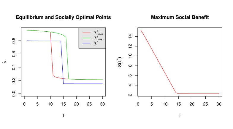
Figure 2: Equilibrium and Socially Optimal rates as a function of $T$ for $R=25$, $\mu_{l}=\frac{1}{4}$.

In Figure 2 we present the results of the sensitivity analysis with respect to the service threshold $T$, for $\mu_{l}=\frac{1}{4}$ and $R=25$. We observe that the equilibrium and optimal arrival rates are decreasing in $T$. This is expected because higher values of the service threshold increase the time that the server spends in the low rate and customers decision to join leads to increased delays due to system congestion, discouraging more customers from joining.

Moreover, for low and high values of $T$, the system behaves approximately as an $M|M|1$ queue with service rate equal to $\mu_{l}$, and $1$, respectively. Therefore, for such $T$ values the equilibrium arrival rate is unique and the optimal arrival rate is lower than the equilibrium because of the negative externalities. On the other hand, for intermediate values of $T$ there are multiple equilibria, as discussed in Section 3. In these cases the optimal rate is between the two extreme values $\lambda^{e}_{\min}$ and $\lambda^{e}_{\max}$ of the equilibrium. Thus, whether the externalities are positive or negative, and thus whether a tax or a subsidy is required to induce efficiency, is not known in advance but it depends on which of the equilibrium rates will materialize. Finally, we observe in Figure 2 that the maximum social benefit $S(\lambda^{*})$ is decreasing in $T$ for fixed values of $R$ and $\mu_{l}$, as a consequence of the behavior of the optimal arrival rate with respect to $T$.

Next, we proceed to numerical results with respect to parameters $R$ and $\mu_{l}$, considering first the case of $T=10$. Using the dynamic service policy $(T,\mu_{l},1)$ for $T=10$ and $\mu_{l}=\frac{1}{5}$, we obtain $\lambda^{*}$ and the corresponding equilibria with respect to $R$, which are illustrated in Figure 3. Note that, the equilibrium analysis for this service policy has been presented in Figure 1(b) and, thus, both diagrams must be considered together, in order to explore the relationship between $\lambda^{*}$ and the equilibria. We see that, $\lambda^{*}\leq\lambda^{e}_{\max}$ for low and high values of the reward, in which case the equilibrium arrival rate is unique, as showed in Figure 1(b). On the other hand, for intermediate values of $R$, where there exist two or three equilibria, we observe that $\lambda^{e}_{\min}\leq\lambda^{*}\leq\lambda^{e}_{\max}$. In this case, customers can impose either positive or negative externalities in equilibrium, as we mentioned before.

Regarding the sensitivity of the social optimal arrival rate and the corresponding equilibria with respect to the low service rate for $R=20$, which is presented in Figure 4, we see that $\lambda^{e}_{\min}\leq\lambda^{*}\leq\lambda^{e}_{\max}$ for low values of $\mu_{l}$, whereas $\lambda^{*}\leq\lambda^{e}_{\max}$ for higher values. This happens because the service rate switch option is no longer beneficial for joining customers, as the low service rate increases to high values. Therefore, the expected waiting time becomes monotone increasing as $\mu_{l}$ increases, corresponding to the delay function of a typical $M|M|1$ queue, which results in the existence of a unique equilibrium strategy with rate larger than $\lambda^{*}$.

Moreover in both figures, we observe that there exist a discontinuity point with respect to $R$ or $\mu_{l}$, which corresponds to the existence of two equal maxima for different values of the reward or the low service rate, respectively. This is due to the fact that the social benefit function $S(\lambda)$ can be bimodal for some values of $R$ or $\mu_{l}$.

Considering the behavior of $\lambda^{*}$ as well as both equilibria, we observe that they are increasing in $R$, which is intuitive considering the fact that customers either as a whole or acting independently are generally better off as the reward increases, and, thus tend to join more. This is also reflected in the behavior of the maximum social benefit $S(\lambda^{*})$, which is always increasing in $R$, as observed in Figure 3.

In contrast, regarding the behavior of the social optimal arrival rate with respect to $\mu_{l}$, we observe in Figure 4 that it is slightly decreasing for small values, and, then becomes increasing, after a discontinuity jump. For this set of values of $T,\;R,\;\mu_{l}$ the social benefit function is bimodal in $\lambda$, with two local maxima. Of these the lower corresponds to a policy that accepts a small proportion of customers and thus keeps delay low by avoiding congestion.

The other local maximum occurs at a higher value of $\lambda$, which means that more customers are accepted, so the server is forced to work at the high rate most of the time, thus keeping the delay moderate. For every value of $\mu_{l}$ one of the two local maxima supersedes the other and determines the optimal value of $\lambda$. For small values of $\mu_{l}$ the lower mode value is so low that almost no one is accepted, thus the higher mode is preferred. On the other hand as $\mu_{l}$ increases, the delay becomes more moderate even when the server works at low rate, which makes the lower mode preferred. The discontinuity point corresponds to the value of $\mu_{l}$ where the two local maxima are equal. As $\mu_{l}$ increases above the discontinuity point, the low mode still persists but nevertheless more customers are accepted under the optimal policy.

Note that regardless of the non-monotone behavior of $\lambda^{*}$, the optimal welfare value $S(\lambda^{*})$ is increasing in $\mu_{l}$, since higher values of this service rate can only improve system performance.

Similar observations can be made for the case $T=3$. For $\mu_{l}=\frac{1}{10}$ and varying $R$, we observe in Figure 5 that $\lambda^{*}\leq\lambda^{e}_{\max}$ for $R<7$ and $R>16$, whereas $\lambda^{e}_{\min}\leq\lambda^{*}\leq\lambda^{e}_{\max}$ for intermediate values of $R$. Moreover, regarding the behavior of the social optimal arrival rate, $\lambda^{*}$ has a discontinuity point in $R=7$. This can be explained by an analogous bimodality argument as in the previous case. In addition, the social optimal arrival rate $\lambda^{*}$, as well as the social optimal benefit $S(\lambda^{*})$, are increasing in $R$ as expected.

We finally note that the discontinuities discussed above do not always occur. For other sets of values of $T,\;R,\;\mu_{l}$, the social welfare function may be unimodal in $\lambda$, or even if it is bimodal one of the two modes may persist as optimal. In these cases the optimal arrival rate is continuous and monotone in the corresponding parameter. For example Figure 6, shows the dependence on $\mu_{l}$ for $T=3$ and $R=5$, where there exists a unique equilibrium for any $\mu_{l}$, which is continuous and increasing in $\mu_{l}$, as is also the socially optimal rate. In this case, the equilibrium is always greater than the socially optimal rate, whenever they take non-zero

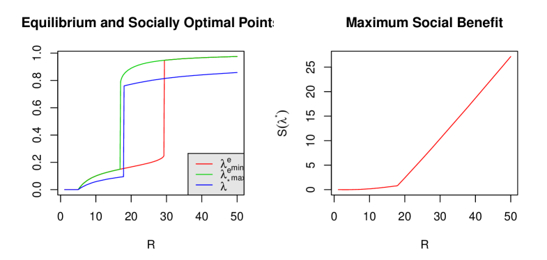
Figure 3: Equilibrium and Socially Optimal rates as a function of $R$ for $T=10$,$\mu_{l}=\frac{1}{5}$.

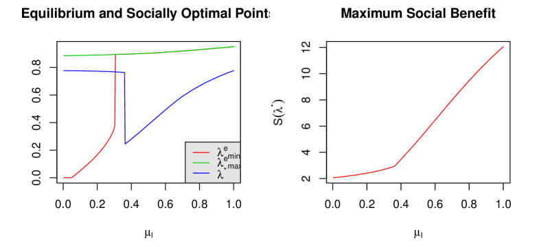
Figure 4: Equilibrium and Socially Optimal rates as a function of $\mu_{l}$ for $T=10$, $R=20$.

Figure 5: Equilibrium and Socially Optimal rates as a function of $R$ for $T=3$, $\mu_{l}=\frac{1}{10}$.

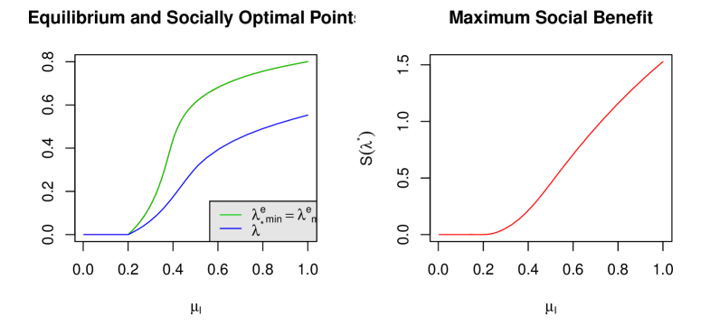
Figure 6: Equilibrium and Socially Optimal rates as a function of $\mu_{l}$ for $T=3$, $R=5$.

5 The Case $T=1$

In this section, we analyze the case where the service threshold $T$ is set to $1$ and, thus the service policy prescribes that the server uses the low rate as long as the queue is empty and switches to the high rate as soon as a customer joins the queue.

This policy may be appropriate when there is a large difference between the two service rate values, and an assurance must be given to the customers that when there is at least one person waiting in the queue the service is expedited.

From the analysis point of view the expressions of the delay function is now considerably simpler, permitting more complete analytical results.

As in the general model, we first characterize the symmetric equilibrium strategies and then proceed to social benefit maximization.

For $T=1$, the delay function in (5) becomes

$$W_{1}(\lambda)=\frac{1}{(1-\lambda)[\mu_{l}+\lambda(1-\mu_{l})]},\;\lambda\in[0,1).$$ (20)

In the following lemma we present some properties of the delay function $W_{1}(\lambda)$. The proof follows from simple calculus and is omitted.

Figure 7: The expected waiting time $W(\lambda)$ for $T=1$ and (a)$\mu_{l}<\frac{1}{2}$ or (b)$\mu_{l}>\frac{1}{2}$

Lemma 2

• $W_{1}(0)=\frac{1}{\mu_{l}}$ and $\lim_{\lambda\rightarrow 1}W_{1}(\lambda)=+\infty$

• If $\mu_{l}>\frac{1}{2}$, $W_{1}(\lambda)$ is increasing in $\lambda\in(0,1)$.

• If $\mu_{l}<\frac{1}{2}$, $W_{1}(\lambda)$ is decreasing in $\lambda\in(0,\frac{1-2\mu_{l}}{2(1-\mu_{l})})$ and is increasing in $\lambda\in(\frac{1-2\mu_{l}}{2(1-\mu_{l})},1)$.

• $W_{1}(\lambda)$ is convex in $\lambda\in(0,1)$.

The plot of $W_{1}(\lambda)$ for two representative values of $\mu_{l}$ is shown in Figure 7.
Equilibrium Analysis For the equilibrium analysis we follow the same steps as in Section 3. Now, equation (12) becomes quadratic:

$$H_{1}(\lambda)=R(1-\mu_{l})\lambda^{2}+R(2\mu_{l}-1)\lambda+1-R\mu_{l}=0.$$ (21)

This equation $H_{1}(\lambda)=0$ can be solved explicitly and may have either one or two roots in $[0,1)$ (the case of zero roots is excluded because of Lemma 1), depending on the values of $R$ and $\mu_{l}$.

Performing a detailed but otherwise standard analysis of the roots, we obtain the following theorem on the number of symmetric equilibria.

Theorem 3

For $\Lambda\geq 1$ the following hold.

• If $R<1$, then $0$ is the unique equilibrium.

• If $1\leq R\leq 2$ and $\mu_{l}\leq\frac{1}{R}$, then $0$ is the unique equilibrium.

• If $R>2$ and $\mu_{l}<1-\frac{R}{4}$, then $0$ is the unique equilibrium.

• If $R>2$ and $\mu_{l}=1-\frac{R}{4}$, then the equilibrium arrival rates are $0$ and $\lambda_{0}^{e}$.

• If $R>2$ and $1-\frac{R}{4}<\mu_{l}<\frac{1}{R}$, then the equilibrium arrival are $0,\;\lambda_{1}^{e}$ and $\lambda_{2}^{e}$.

• If $R\geq 1$ and $\mu_{l}>\frac{1}{R}$, then $\lambda_{1}^{e}$ is the unique equilibrium.

where

$$\lambda_{1}^{e}=\frac{R(1-2\mu_{l})+\sqrt{R(R-4(1-\mu_{l}))}}{2R(1-\mu_{l})},$$ (22)

$$\lambda_{2}^{e}=\frac{R(1-2\mu_{l})-\sqrt{R(R-4(1-\mu_{l}))}}{2R(1-\mu_{l})}$$ (23)

and

$$\lambda_{0}^{e}=\frac{(1-2\mu_{l})}{2(1-\mu_{l})}.$$ (25)

In Figure 8 we present the number of symmetric equilibria in different regions of the $R-\mu_{l}$ plane, corresponding to the cases listed in Theorem 3.

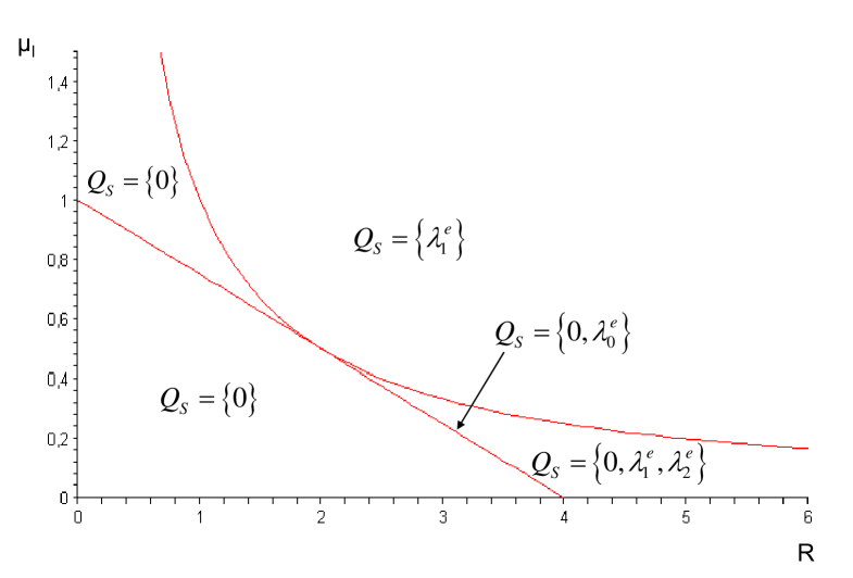
Figure 8: Symmetric Equilibria for the Case T=1, for several values of the parameters $\mu_{l}$ and $R$

Social Optimization Proceeding to the social optimization problem, we let $S_{1}(\lambda)$ be the social welfare function in the case of $T=1$. Thus,

$$S_{1}(\lambda)=\lambda\left[R-W_{1}(\lambda)\right],$$ (26)

In the following lemma we derive some properties of $S_{1}(\lambda)$.

Lemma 3

• If $\mu_{l}<\frac{1}{2}$, then $S_{1}(\lambda)$ is strictly concave in $\lambda\in[0,1)$.

• If $\mu_{l}=1-\frac{R}{4}<\frac{1}{2}$, then $S_{1}(\lambda)$ is decreasing and concave in $\lambda\in(\lambda_{0}^{e},1)$.

• If $1-\frac{R}{4}<\mu_{l}<\frac{1}{2}$, then $S_{1}(\lambda)$ is decreasing and concave in $\lambda\in(\lambda_{1}^{e},1)$.

Proof   The first two derivatives of $S_{1}(\lambda)$ are

$$S_{1}^{\prime}(\lambda)=R-W_{1}(\lambda)-\lambda W_{1}^{\prime}(\lambda)$$ (27)

$$S_{1}^{\prime\prime}(\lambda)=-2W_{1}^{\prime}(\lambda)-\lambda W_{1}^{\prime\prime}(\lambda).$$ (28)

i. If $\mu>\frac{1}{2}$, $W_{1}(\lambda)$ is increasing and convex in $\lambda\in[0,1)$, as stated in Lemma 2. By (28), it follows that $S_{1}^{\prime\prime}(\lambda)<0\;\forall\lambda\in[0,1)$, and the statement holds.

ii. The expression of $S_{1}^{\prime}(\lambda)$ in (27) can be rewritten as

$$S_{1}^{\prime}(\lambda)=-\frac{H_{1}(\lambda)}{(1-\lambda)(\mu_{l}+(1-\mu_{l})\lambda)}-\lambda W_{1}^{\prime}(\lambda)$$ (29)

where $H_{1}(\lambda)$ is the polynomial in (21).

Now, for $\mu_{l}=1-\frac{R}{4}<\frac{1}{2}$, we obtain that $H_{1}(\lambda)>0,\;\forall\lambda\in[0,\lambda_{0}^{e})\cup(\lambda_{0}^{e},1)$. Also, $W_{1}(\lambda)$ is increasing in $\lambda\in(\lambda_{0}^{e},1)$. By (29) and (28) we obtain that $S_{1}^{\prime}(\lambda)<0$ and $S_{1}^{\prime\prime}(\lambda)<0$ for $\lambda\in(\lambda_{0}^{e},1)$. Thus, $S_{1}(\lambda)$ is decreasing and concave in $\lambda\in(\lambda_{0}^{e},1)$.

iii. Similarly to ii. it can be shown that $S_{1}(\lambda)$ is decreasing and concave in $\lambda\in(\lambda_{1}^{e},1)$.   
In the following proposition we prove a result on the relationship between the optimal and equilibrium arrival rates. In this case, $\lambda^{e}$ refers to a positive and stable equilibrium arrival rate.

Proposition 2

For any $\mu_{l}\in(0,1)$ and $R\geq 1$ there exists an equilibrium $\lambda^{e}$ such that $\lambda^{*}\leq\lambda^{e}$ for any social optimal arrival rate $\lambda^{*}\in[0,1)$.

Proof   In order to prove the statement of Proposition 2 we consider the cases of Lemma 3 for the value of $\mu_{l}$.

First, assume $\mu_{l}>\frac{1}{2}$. By the concavity of the social welfare function $S_{1}(\lambda)$, as stated in Lemma 3, it follows that there exists a unique social optimal arrival rate $\lambda^{*}$, which maximizes $S_{1}(\lambda)$.

In addition, if $\mu_{l}\leq\frac{1}{R}$ the unique equilibrium arrival rate is $\lambda^{e}=0$ with $S_{1}^{\prime}(0)=R-W(0)=R-\frac{1}{\mu_{l}}\leq 0$. Thus, $S_{1}^{\prime}(0)\leq S_{1}^{\prime}(\lambda^{*})$ and by the monotonicity of $S_{1}^{\prime}(\lambda)$ we obtain that $\lambda^{*}\leq 0$, which results to $\lambda^{*}=0$. If, on the contrary, $\mu_{l}>\frac{1}{R}$, the unique equilibrium arrival rate is $\lambda^{e}=\lambda^{e}_{1}$ with $S_{1}^{\prime}(\lambda^{e}_{1})<0$. Once again, by the monotonicity of $S_{1}^{\prime}(\lambda)$ we prove that $\lambda^{*}\leq\lambda^{e}$ for any $\lambda^{*}$.

Next, we consider the case where $\mu_{l}=1-\frac{R}{4}<\frac{1}{2}$. By Lemma 3, we obtain that $S_{1}(\lambda)$ is decreasing and concave in $\lambda\in(\lambda_{0}^{e},1)$. Thus, $\lambda^{*}\leq\lambda_{0}^{e}$ for any $\lambda^{*}$, where $\lambda_{0}^{e}$ is the stable and positive equilibrium arrival rate, as stated in Proposition 3.

Finally, for the case of $1-\frac{R}{4}<\mu_{l}<\frac{1}{2}$, it follows similarly that $\lambda^{*}\leq\lambda_{1}^{e}$ for any optimal arrival rate $\lambda^{*}$, where $\lambda_{1}^{e}$ is the stable positive equilibrium arrival rate.   

6 Conclusions and Extensions

In this paper, we considered the problem of customer equilibrium joining behavior in an unobservable $M|M|1$ queue with dynamically adjusted service rate according to a threshold type service policy, known to all customers. We proved that there exist multiple equilibria, three at most, due to the presence of both positive and negative externalities for different values of the effective arrival rate. For the social welfare optimization problem, we explored the relationship between the optimal and the equilibrium arrival rates in several numerical experiments for different values of system parameters. We demonstrated that in cases where there exist multiple equilibria, the socially optimal point lies between the extreme equilibrium values, whereas in all other cases it is always less than the equilibrium arrival rate.

This work can be extended in several directions. First, it would be of interest to determine the equilibrium strategies under different levels of information on system congestion or the status of the server upon customer arrival. Some preliminary work has shown that the equilibrium analysis in these problems is significantly more complex, and non-threshold equilibria may exist. In terms of the form of the service control policy, one might consider an alternative where instead of increasing the service speed with congestion, one or more standby servers are activated. Such a policy is more relevant in situations where the service is provided by human workers. Other extensions include generally distributed service requirements and dynamic service speed, series of queues with different parameters and/or service policies, and systems where the specific service policy threshold is not announced to the customers.

References

- (1)
- Adusumilli & Hasenbein (2010) Adusumilli, K. & Hasenbein, J. (2010), ‘Dynamic admission and service rate control of a queue’, Queueing Systems 66, 131–154.
- Armony & Maglaras (2004) Armony, M. & Maglaras, C. (2004), ‘Contact centers with a call-back option and real-time delay information.’, Operations Research 52(4), 527–545.
- Ata & Shneorson (2006) Ata, B. & Shneorson, S. (2006), ‘Dynamic control of an m/m/1 service system with adjustable arrival and service rates’, Manage. Sci. 52(11), 1778–1791.
- Burnetas & Economou (2007) Burnetas, A. & Economou, A. (2007), ‘Equilibrium customer strategies in a single server markovian queue with setup times.’, Queueing Systems 56(3-4), 213–228.
- Chen & Frank (2004) Chen, H. & Frank, M. (2004), ‘Monopoly pricing when customers queue’, IEE Transactions 36, 569–581.
- Debo & Veeraraghavan (2009) Debo, L. G. & Veeraraghavan, S. K. (2009), ‘Joining longer queues: Information externalities in queue’, Manufacturing, Services and Operations Management Science 11, 543–562.
- Dimitrakopoulos & Burnetas (2011) Dimitrakopoulos, Y. & Burnetas, A. (2011), The value of service rate flexibility in an M/M/1 queue with admission control. Working Paper.
- Economou & Manou (2011) Economou, A. & Manou, A. (2011), ‘Equilibrium balking strategies for a clearing queueing system in alternating environment’, Annals of Operations Research . to appear.
- Edelson & Hildebrand (1975) Edelson, N. & Hildebrand, D. (1975), ‘Congestion tolls for poisson queueing processes.’, Econometrica 43, 81–92.
- George & Harrison (2001) George, J. M. & Harrison, J. M. (2001), ‘Dynamic control of a queue with adjustable service rate’, Operations Research 49(5), 720–731.
- Guo & Hassin (2011) Guo, P. & Hassin, R. (2011), ‘Strategic behavior and social optimization in markovian vacation queues’, Operations Research 59(4), 986–997.
- Hassin & Haviv (2003) Hassin, R. & Haviv, M. (2003), To queue or not to queue: Equilibrium behavior in queueing systems., Springer.
- Naor (1969) Naor, P. (1969), ‘On the regulation of queue size by levying tolls’, Econometrica 37, 15–24.
- Stenbacka & Tombak (1995) Stenbacka, R. & Tombak, M. M. (1995), ‘Time-based competition and privatization of services’, The Journal of Industrial Economics 43, 435–454.
- Wilf (1962) Wilf, H. (1962), Mathematics for the Physical Sciences, Dover Pub. Inc.