Connectivity and Set Tracking of Multi-agent Systems Guided by Multiple Moving Leaders

Abstract

In this paper, we investigate distributed multi-agent tracking of a convex set specified by multiple moving leaders with unmeasurable velocities. Various jointly-connected interaction topologies of the follower agents with uncertainties are considered in the study of set tracking. Based on the connectivity of the time-varying multi-agent system, necessary and sufficient conditions are obtained for set input-to-state stability and set integral input-to-state stability for a nonlinear neighbor-based coordination rule with switching directed topologies. Conditions for asymptotic set tracking are also proposed with respect to the polytope spanned by the leaders.

Keywords. Multi-agent systems, multiple leaders, set input-to-state stability (SISS), set integral input-to-state stability (SiISS), set tracking.

1 Introduction

The last decade has witnessed tremendous interest devoted to the investigation of collective phenomena in multiple autonomous agents, due to broad applications in various fields of science ranging from biology to physics, engineering, and ecology, just to name a few [8, 9, 10, 11, 12]. Concerning the issues of multi-agent systems and distributed design, the revolutionary idea is underpinning a strong interaction of individual dynamics, communication topologies, and distributed controls. The problem is generally very challenging due to the complex dynamics and hierarchical structures of the systems. However, efforts have been started with relatively simple problems such as consensus, formation, and rendezvous, and many significant results have been obtained.

The leader-follower coordination is an important multi-agent control problem, where the leader may be a real leader (such as a target, an evader, or a predefined position), or a virtual leader (such as a reference trajectory or a specified path). In most theoretical work, a single leader with exact measurement is considered on multi-agent systems for each agent to follow. However, in practical situations, multiple leaders and target sets with unmeasurable variables are considered to achieve desired collective behaviors. In [8], a simple model was given to simulate fish foraging and demonstrate the leader effectiveness when the leaders (or informed agents) guide a school of fish to a particular food region. In [23], a straight-line formation of a group of agents was discussed, where all the agents converge to the line segment specified by two edge leaders. A containment control scheme was proposed with fixed undirected interaction in [24], which aimed at driving a group of agents to a given target location and making their positions contained in the polytope spanned by multiple stationary or moving leaders during their motion. Region following formation control was constructed [25], where all the robots are driven and then stay within a moving target region as a group. Moreover, different dynamic connectivity conditions were obtained to guarantee that the multiple leaders (or informed agents) aggregate the whole multi-agent group within a convex target set in [26]. Additionally, control strategies were demonstrated and analyzed to drive a collection of mobile agents to stationary/moving leaders with connectivity-maintenance and collision-avoidance with fixed and switching directed network topologies in [27]. As a matter of fact, multiple leaders are usually assigned to increase control effectiveness, enhance communication/sensing range, improve reliability, and optimize energy cost in multi-agent coordination.

Connectivity plays a key role in the coordination of multi-agent networks, which is related to the influence of agents and controllability of the network. Due to mobility of the agents, inter-agent topologies usually keep changing in practice. Therefore, the various connectivity conditions to describe frequently switching topologies in order to deal with multi-agent consensus or flocking [15, 16, 18, 21]. In fact, the “joint connection” or similar concepts are important in the analysis of stability and convergence to guarantee multi-agent coordination with time-dependent topology. Uniformly jointly-connected conditions have been employed for different problems. [28] studied the distributed asynchronous iterations, while [22] proved the consensus of a simplified Vicsek model. Furthermore, [14] and [6] investigated the jointly-connected coordination for second-order agent dynamics via different approaches, while [30] worked on nonlinear continuous-time agent dynamics with jointly-connected interaction graphs. Also, flocking of multi-agent system with state-dependent topology was studied with non-smooth analysis in [18, 20]. What is more, the $[t,\infty)$ joint connection condition, which is more generalized than the uniformly joint connection assumption, was discussed by Moreau, in order to achieve the consensus for discrete-time agents in [31]. This $[t,\infty)$ connectivity concept was then extended in the distributed control analysis for the target set convergence in [26].

It is well known that input-to-state stability (ISS) is an important and very useful tool in the study of the stability and stabilization of control systems [29, 35]. Its variants such as integral input-to-state stability (iISS) were discussed in [34]. Then few works on set input-to-state stability (SISS) were done with respect to fixed sets in [33]. On the other hand, ISS or related ideas can facilitate the control analysis and synthesis with interconnection conditions like small gains (referring to [29], for example). ISS has recently been applied to the stability study of a group of interconnected nonlinear systems [32]. Moreover, an extended concept called leader-to-formation stability was introduced to investigate the stability of the formation of a group of agents in light of ISS properties [19]. In fact, ISS application in multi-agent systems is promising.

The contributions of the paper include:

• We propose the generalized set input-to-state stability (SISS) and set integral-input-to-state stability (SiISS) to handle moving sets with time-varying shapes for switching multi-agent networks.

• We study the multi-leader coordination from the ISS viewpoint. With the help of SISS and SiISS, we give explicit expressions to estimate the convergence rate and tracking error of a group of mobile agents that try to enter the convex hull determined by multiple leaders.

• We show relationships between the connectivity and set tracking of the multi-agent system, and find that various jointly-connected conditions usually provide necessary and/or sufficient conditions for distributed coordination.

• We develop a method to study SISS and SiISS for a moving set and switching topology with graph theory and non-smooth analysis. In fact, we cannot take the standard approaches to conventional ISS or iISS using equivalent ISS-Lyapunov functions [34, 35]. In addition, the classic algebraic methods based on Laplacian may fail due to disturbances in nonlinear agent dynamics, uncertain leader velocities, or moving multi-leader set.

This paper is organized as follows. Section 2 presents the preliminaries and problem formulation, while Section 3 proposes results for the convergence estimation. Section 4 mainly reports a necessary and sufficient condition for the SISS with respect to the moving multi-leader set with switching inter-agent topologies, and then presents a set-tracking case based on the SISS. Correspondingly, Section 5 obtains necessary and sufficient conditions for SiISS and then shows set-tracking results related to SiISS. Finally, Section 6 gives concluding remarks.

2 Problem Formulation

In this section, we introduce some preliminary knowledge for the following discussion.

First we introduce some basic concepts in graph theory (referring to [13] for details). A directed graph (digraph) $\mathcal{G}=(\mathcal{V},\mathcal{E})$ consists of a finite set $\mathcal{V}=\{1,2,...,n\}$ of nodes and an arc set $\mathcal{E}$, in which an arc is an ordered pair of distinct nodes of $\mathcal{V}$. $(i,j)\in\mathcal{E}$ describes an arc which leaves $i$ and enters $j$. A walk in digraph $\mathcal{G}$ is an alternating sequence $\mathcal{W}:i_{1}e_{1}i_{2}e_{2}\dots e_{m-1}i_{m}$ of nodes $i_{\kappa}$ and arcs $e_{\kappa}=(i_{\kappa},i_{\kappa+1})\in\mathcal{E}$ for $\kappa=1,2,\dots,m-1$. A walk is called a path if the nodes of this walk are distinct, and a path from $i$ to $j$ is denoted as $\widehat{(i,j)}$. Node $j$ is called reachable from $i$ if there is a path $\widehat{(i,j)}$. If the nodes $i_{1},\dots,i_{m-1}$ are distinct and $i_{1}=i_{m}$, $\mathcal{W}$ is called a (directed) cycle. A digraph without cycles is said to be acyclic.

The union of the two digraphs $\mathcal{G}_{1}=(\mathcal{V},\mathcal{E}_{1})$ and $\mathcal{G}_{2}=(\mathcal{V},\mathcal{E}_{2})$ is defined as $\mathcal{G}_{1}\cup\mathcal{G}_{2}=(\mathcal{V},\mathcal{E}_{1}\cup\mathcal{E}_{2})$ if they have the same node set. Furthermore, a time-varying digraph is defined as $\mathcal{G}_{\sigma(t)}=(\mathcal{V},\mathcal{E}_{\sigma(t)})$ with $\sigma:t\rightarrow\mathcal{Q}$ as a piecewise constant function, where $\mathcal{Q}$ is the finite set which consists of all the possible digraphs with node set $\mathcal{V}$. Moreover, the joint digraph of $\mathcal{G}_{\sigma(t)}$ in time interval $[t_{1},t_{2})$ with $t_{1}<t_{2}\leq+\infty$ is denoted as

$$\mathcal{G}([t_{1},t_{2}))=\cup_{t\in[t_{1},t_{2})}\mathcal{G}(t)=(\mathcal{V},\cup_{t\in[t_{1},t_{2})}\mathcal{E}_{\sigma(t)}).$$ (1)

Next, we recall some notations in convex analysis (see [2]). A set $K\subset R^{d}$ is said to be convex if $(1-\lambda)x+\lambda y\in K$ whenever $x\in K,y\in K$ and $0\leq\lambda\leq 1$. For any set $S\subset R^{d}$, the intersection of all convex sets containing $S$ is called the convex hull of $S$, denoted by $co(S)$. Particularly, the convex hull of a finite set of points $x_{1},\dots,x_{n}\in R^{d}$ is a polytope, denoted by $co\{x_{1},\dots,x_{n}\}$. In fact, we have $co\{x_{1},\dots,x_{n}\}=\{\lambda_{1}x_{1}+\dots+\lambda_{n}x_{n}|\lambda_{1}+\dots+\lambda_{n}=1,\lambda_{i}\geq 0\}$.

Let $K$ be a closed convex subset in $R^{d}$ and denote $|x|_{K}\triangleq\inf\{|x-y|\mid y\in K\}$, where $|\cdot|$ denotes the Euclidean norm for a vector or the absolute value of a scalar ([35, 34]). Then we can associate to any $x\in R^{d}$ a unique element $\mathcal{P}_{K}(x)\in K$ satisfying $|x-\mathcal{P}_{K}(x)|=|x|_{K},$ where the map $\mathcal{P}_{K}$ is called the projector onto $K$ and

$$\langle\mathcal{P}_{K}(x)-x,\mathcal{P}_{K}(x)-y\rangle\leq 0,\quad\forall y\in K.$$ (2)

Clearly, $|x|_{K}^{2}$ is continuously differentiable at point $x$, and (see [1])

$$\nabla|x|_{K}^{2}=2(x-\mathcal{P}_{K}(x)).$$ (3)

The following lemma was obtained in [26], which is useful in what follows.

Lemma 2.1

Suppose $K\subset R^{d}$ is a convex set and $x_{a},x_{b}\in R^{d}$. Then

$$\langle x_{a}-\mathcal{P}_{K}(x_{a}),x_{b}-x_{a}\rangle\leq|x_{a}|_{K}\cdot\left.||x_{a}|_{K}-|x_{b}|_{K}\right|.$$ (4)

Particularly, if $|x_{a}|_{K}>|x_{b}|_{K}$, then

$$\langle x_{a}-\mathcal{P}_{K}(x_{a}),x_{b}-x_{a}\rangle\leq-|x_{a}|_{K}\cdot(|x_{a}|_{K}-|x_{b}|_{K}).$$ (5)

Then we consider the Dini derivative for the following non-smooth analysis. Let $a$ and $b\;(>a)$ be two real numbers and consider a function $h:(a,b)\to R$ and a point $t\in(a,b)$. The upper Dini derivative of $h$ at $t$ is defined as

$$D^{+}h(t)=\limsup_{s\to 0^{+}}\frac{h(t+s)-h(t)}{s}.$$

It is well known that when $h$ is continuous on $(a,b)$, $h$ is non-increasing on $(a,b)$ if and only if $D^{+}h(t)\leq 0$ for any $t\in(a,b)$ (more details can be found in [3]). The next result is given for the calculation of Dini derivative [4, 30].

Lemma 2.2

Let $V_{i}(t,x):R\times R^{d}\to R\;(i=1,\dots,n)$ be $C^{1}$ and $V(t,x)=\max_{i=1,\dots,n}V_{i}(t,x)$. If $\mathcal{I}(t)=\{i\in\{1,2,\dots,n\}\,:\,V(t,x(t))=V_{i}(t,x(t))\}$ is the set of indices where the maximum is reached at $t$, then $D^{+}V(t,x(t))=\max_{i\in\mathcal{I}(t)}\dot{V}_{i}(t,x(t)).$

In this paper, we consider the set coordination problems for a multi-agent system consisting of $n$ follower-agents and $k$ leader-agents (see Fig. 1). The follower set is denoted as $\mathcal{V}_{F}\triangleq\{v_{1},\dots,v_{n}\}$, and the leader set is denoted as $\mathcal{V}_{L}\triangleq\{\hat{v}_{1},\dots,\hat{v}_{k}\}$. In what follows, we will identify follower $v_{i}$ or leader $\hat{v}_{i}$ with its index $i$ (namely, agent $i$ or leader $i$) if there is no confusion.

Then we describe the communication in the multi-agent network. At time $t$, if $i\in\mathcal{V}_{F}$ can “see” $j\in\mathcal{V}_{F}$, there is an arc $(j,i)$ (marking the information flow) from $j$ to $i$, and then agent $j$ is said to be a neighbor of agent $i$. Moreover, if $i\in\mathcal{V}_{F}$ “sees” $j\in\mathcal{V}_{L}$ at time $t$, there is an arc $(j,i)$ leaving from $j$ and entering $i$, and then $j$ is said to be a leader of agent $i$. Let $N_{i}$ and $L_{i}$ represent the set of agent $i$’s neighbors and the set of agent $i$’s leaders (that is, the leaders which are connected to agent $i$), respectively. Note that, since the leaders are not influenced by the followers, there is no arc leaving from $\mathcal{V}_{F}$ entering $\mathcal{V}_{L}$.

Figure 1: Multiple agents ($v_{i},\,i=1,2,3,4$) with multiple leaders ($\hat{v}_{i},\,i=1,2,3$)

Define $\mathcal{V}=\mathcal{V}_{F}\cup\mathcal{V}_{L}$ as the whole agent set (including leaders and followers). Denote $\mathcal{P}$ as the set of all possible interconnection topologies, and $\sigma:[0,+\infty)\rightarrow\mathcal{P}$ as a piecewise constant switching signal function to describe the switchings between the topologies. Thus, the interaction topology of the considered multi-agent network is described by a time-varying directed graph $\mathcal{G}_{\sigma(t)}=(\mathcal{V},\mathcal{E}_{\sigma(t)})$. Correspondingly, $\mathcal{G}^{F}_{\sigma(t)}$ is denoted as the communication graph among the follower agents. Additionally, let $N_{i}(\sigma(t))$ and $L_{i}(\sigma(t))$ represent the set of agent $i$’s neighbors and the set of its connected leaders in $\mathcal{G}_{\sigma(t)}$, respectively.

As usual in the literature [22, 30, 26], an assumption is given for the switching signal $\sigma(t)$.

Assumption 1 (Dwell Time) There is a lower bound $\tau_{D}>0$ between two switching instants.

We give definitions for the connectivity of a multi-agent system with multiple leaders.

Definition 2.1

(i) $\mathcal{G}_{\sigma(t)}$ is said to be L-connected if, for any $i\in\mathcal{V}_{F}$, there exists a leader $j\in\mathcal{V}_{L}$ such that there is a path from leader $j$ to agent $i$ in $\mathcal{G}_{\sigma(t)}$ at time $t$. Moreover, $\mathcal{G}_{\sigma(t)}$ is said to be jointly L-connected in time interval $[t_{1},t_{2})$ if the union graph $\mathcal{G}([t_{1},t_{2}))$ is L-connected;

(ii) $\mathcal{G}_{\sigma(t)}$ is said to be jointly L-connected (JLC) if the union graph $\mathcal{G}([t,\infty))$ is L-connected for any $t$;

(iii) $\mathcal{G}_{\sigma(t)}$ is said to be uniformly jointly L-connected (UJLC) if there exists $T>0$ such that the union graph $\mathcal{G}([t,t+T))$ is L-connected for any $t\geq 0$.

Remark 2.1

Note that the L-connectedness describes the capacity for the follower agents to get the information from the moving multi-leader set in the information flow, and an L-connected graph may not be connected since the graph with leaders as its nodes may not be connected. In fact, if we consider the group of the leaders as one virtual node in $\mathcal{V}$, then the L-connectedness becomes the quasi-strong connectedness for a digraph [5, 30].

The state of agent $v_{i}\in\mathcal{V}_{F}$, is denoted as $x_{i}\in R^{d}\,(i=1,\dots,n$), and the state of leader $\hat{v}_{i}\in\mathcal{V}_{L}$, is denoted as $y_{i}\in R^{d}\,(i=1,\dots,k$). Denote $x=(x_{1},\dots,x_{n})^{T}\in R^{nd}$ and $y=(y_{1},\dots,y_{k})^{T}\in R^{kd}$ and let the continuous function $a_{ij}(x,y,t)>0$ be the weight of arc $(j,i)$, if any, for $i,j\in\mathcal{V}_{F}$, and continuous function $b_{ij}(x,y,t)>0$ be the weight of arc $(j,i)$, if any, for $i\in\mathcal{V}_{F};j\in\mathcal{V}_{L}$.

Then we present the multi-agent model for the active leaders and the (follower) agents

$$\left\{\begin{array}[]{ll}\dot{y}_{i}=u_{i}(y,t),\quad\quad i=1,\dots,k\\ \dot{x}_{i}=\sum\limits_{j\in N_{i}(\sigma(t))}a_{ij}(x,y,t)(x_{j}-x_{i})+\sum\limits_{j\in L_{i}(\sigma(t))}b_{ij}(x,y,t)(y_{j}-x_{i})+w_{i}(t),\;\quad i=1,\dots,n\end{array}\right.$$ (6)

where $u_{i}(y,t)$ describes the control inputs of the leader $i,i\in\mathcal{V}_{L}$, which is continuous in $y$ for fixed $t$ and piecewise continuous in $t$ for fixed $y$, and $w_{i}(t)$ is a continuous function to describe the disturbances in communication links and individual dynamics to follower agent $i$. Then another assumption is given on the weight functions $a_{ij}(x,y,t)$ and $b_{ij}(x,y,t)$.

Assumption 2 (Bounded Weights) There are $0<a_{\ast}\leq a^{\ast}$ and $b_{\ast}>0$ such that $a_{\ast}\leq a_{ij}(x,y,t)\leq a^{\ast},\;b_{\ast}\leq b_{ij}(x,y,t)$ for any $x,y,t$.

Remark 2.2

In (6), the weights, $a_{ij}$ and $b_{ij}$, may not be constant. Instead, because of the complex communication and environment uncertainties, they are dependent on time or space or relative measurement (see nonlinear models given in [30, 26, 31, 18]). Some models such as those studied in [30, 26] can be written in the form of (6), while other nonlinear multi-agent models may be transformed to this class of multi-agent systems in some situations. Here $a_{ij}(x,y,t)$ and $b_{ij}(x,y,t)$ are written in a general form simply for convenience, and global information is not required in our study. For example, $a_{ij}$ and $b_{ij}$ can depend only on the state of $x_{i}$, time $t$ and $x_{j}\,(j\in N_{i})$, which is certainly a special form of $a_{ij}(x,y,t)$ or $b_{ij}(x,y,t)$. In other words, the control laws in specific decentralized forms are still decentralized.

Without loss of generality, we assume the initial time $t=0$, and the initial condition $x^{0}=(x_{1}(0),\dots,x_{n}(0))^{T}\in R^{nd}$ and $y^{0}=(y_{1}(0),\dots,y_{k}(0))^{T}\in R^{kd}$.

Denote the time-varying polytope formed by the $k$ active leaders

$$\mathcal{L}(y(t))\triangleq co\{y_{1}(t),\dots,y_{k}(t)\},$$ (7)

and let

$$|x(t)|_{\mathcal{L}(y(t))}\triangleq\max_{i\in\mathcal{V}_{F}}|x_{i}(t)|_{\mathcal{L}(y(t))}$$

be the maximal distance for the followers away from the moving multi-leader set $\mathcal{L}(y(t))$.

The following definition is to describe the convergence to the moving convex set $\mathcal{L}(y(t))$.

Definition 2.2

The (global) set tracking (ST) with respect to ${\cal L}(y(t))$ for system (6) is achieved if

$$\lim_{t\rightarrow+\infty}|x(t)|_{\mathcal{L}(y(t))}=0$$ (8)

for any initial condition $x^{0}\in R^{nd}$ and $y^{0}\in R^{kd}$.

For a stationary convex set $K$, set tracking can be reduced to set stability and attractivity, and methods to analyze $|x_{i}(t)|_{K}$ were proposed in some existing works [26]. In fact, [24, 27] discussed the convergence to the static convex set determined by stationary leaders with well designed control protocols. Moreover, if we assume that the target set is exactly the polytope with the positions of the stationary leaders (or informed agents) as its vertices, then the convergence to the polytope, treated as a target set, can be obtained straightforwardly based on the results and limit-set-based methods given in [26].

Input-to-state stability has been widely used in the stability analysis and set input-to-state stability (SISS) for a fixed set has been studied in [33]. To study the multi-leader set tracking in a broad sense, we introduce a generalized SISS with respect to $\mathcal{L}(y(t))$, a moving set with a time-varying shape, for multi-agent systems with switching interaction topologies. Denote $u\triangleq(u_{1},\dots,u_{k})^{T}$, $w\triangleq(w_{1},\dots,w_{n})^{T}$, $z\triangleq(u^{T}\;w^{T})^{T}$, and $L_{\infty}\triangleq\{z:R_{\geq 0}\rightarrow R^{(n+k)m}\;|\,\|z\|_{\infty}<\infty\}$ with $\|z\|_{\infty}\triangleq\sup\{|z(t)|,t\geq 0\}$ ([35]).

A function $\gamma:R_{\geq 0}\rightarrow R_{\geq 0}$ is said to be a $\mathcal{K}$-class function if it is continuous, strictly increasing, and $\gamma(0)=0$. Moreover, a function $\beta:R_{\geq 0}\times R_{\geq 0}\rightarrow R$ is a $\mathcal{KL}$-class function if $\beta(\cdot,t)$ is of class $\mathcal{K}$ for each fixed $t\geq 0$ and $\beta(s,t)$ decreases to $0$ as $t\rightarrow\infty$ for each fixed $s\geq 0$.

Definition 2.3

System (6) is said to be globally generalized set input-to-state stable (SISS) with respect to ${\cal L}(y(t))$ with input $z$ if there exist a $\mathcal{K}\mathcal{L}$-function $\beta$ and a $\mathcal{K}$-function $\gamma$ such that

$$|x(t)|_{\mathcal{L}(y(t))}\leq\beta(|x^{0}|_{\mathcal{L}(y^{0})},t)+\gamma(\|z\|_{\infty})$$ (9)

for $z\in L_{\infty}$ and any initial conditions $x^{0}\in R^{nd}$ and $y^{0}\in R^{kd}$.

Integral-input-to-state stability (iISS) was introduced as an integral variant of ISS, which has been proved to be strictly weaker than ISS [34]. We also introduce a definition of (generalized) set integral-input-to-state stability (SiISS) with respect to a time-varying and moving set.

Definition 2.4

System (6) is (globally) generalized set integral-input-to-state stable (SiISS) with respect to ${\cal L}(y(t))$ if there exist a $\mathcal{K}\mathcal{L}$-function $\beta$ and a $\mathcal{K}$-function $\gamma$ such that

$$|x(t)|_{\mathcal{L}(y(t))}\leq\beta(|x^{0}|_{\mathcal{L}(y^{0})},t)+\int_{0}^{t}\gamma(|z(s)|)ds,$$ (10)

for any initial conditions $x^{0}\in R^{nd}$ and $y^{0}\in R^{kd}$.

The conventional SISS was given for a fixed set $K$ ([33]), while the generalized SISS or SiISS is proposed with respect to a time-varying set $\mathcal{L}(y(t))$. In the following, we still use SISS or SiISS instead of generalized SISS or SiISS for simplicity.

Remark 2.3

Similar to the study of conventional ISS, local SISS and SiISS can be defined. In this paper, we focus on the global SISS and SiISS. In fact, it is rather easy to extend research ideas of global set tracking to study local cases.

3 Convergence Estimation

For the set tracking with respect to a moving multi-leader set of system (6), we have to deal with the estimation of $|x_{i}(t)|_{\mathcal{L}(y(t))}$ when $\mathcal{L}(y(t))$ is a time-varying convex set, where $y(t)$ is a trajectory of the moving leaders in system (6) with initial condition $y^{0}=y(0)$. Define

$$r(t)\triangleq\max_{i\in\mathcal{V}_{L}}|u_{i}(y(t),t)|;\quad q(t)\triangleq\max_{i\in\mathcal{V}_{L}}|u_{i}(y(t),t)|+\max_{i\in\mathcal{V}_{F}}|w_{i}(t)|.$$ (11)

Obviously,

$$q(t)\leq|u(y(t),t)|+|w(t)|\leq\sqrt{2}|z(t)|\leq\sqrt{2}\max\{\sqrt{n},\sqrt{k}\}q(t).$$ (12)

The following result is given to estimate the changes of the distance between an agent and the convex hull spanned by the leaders.

Lemma 3.1

For any $t,t_{0}\geq 0$ and $i=1,\dots,n$,

$$||x_{i}(t)|_{\mathcal{L}(y(t))}-|x_{i}(t)|_{\mathcal{L}(y(t_{0}))}|\leq\int_{t_{0}}^{t}r(s)ds.$$ (13)

Proof: Suppose

$$\mathcal{P}_{\mathcal{L}(y(t_{0}))}(x_{i}(t))=\sum_{i=1}^{k}\lambda_{i}y_{i}(t_{0})\in\mathcal{L}(y(t_{0})),$$

where $\lambda_{i}\geq 0$ for $i=1,\dots,k$ with $\sum\limits_{i=1}^{k}\lambda_{i}=1$. Define $\hat{y}(t)\triangleq\sum\limits_{i=1}^{k}\lambda_{i}y_{i}(t)$, and then

$$|\hat{y}(t)-\hat{y}(t_{0})|\leq\sum_{i=1}^{k}\lambda_{i}|y_{i}(t)-y_{i}(t_{0})|=\sum_{i=1}^{k}\lambda_{i}|\int_{t_{0}}^{t}u_{i}(y(s),s)ds|\leq\int_{t_{0}}^{t}r(s)ds$$

Moreover,

$$|x_{i}(t)|_{\mathcal{L}(y(t))} \leq |x_{i}(t)-\hat{y}(t)|$$ (14)

$$\leq |x_{i}(t)-\hat{y}(t_{0})|+|\hat{y}(t)-\hat{y}(t_{0})|$$

$$\leq |x_{i}(t)|_{\mathcal{L}(y(t_{0}))}+\int_{t_{0}}^{t}r(s)ds$$

Also, similar analysis leads to

$$|x_{i}(t)|_{\mathcal{L}(y(t_{0}))}\leq|x_{i}(t)|_{\mathcal{L}(y(t))}+\int_{t_{0}}^{t}r(s)ds$$ (15)

Therefore, (14) and (15) lead to the conclusion. $\square$

For simplicity, define $\psi_{i}(t)\triangleq|x_{i}(t)|^{2}_{\mathcal{L}(y(t))},\;i=1,\dots,n$ and

$$\Psi(t)\triangleq\max_{i\in\mathcal{V}_{F}}\psi_{i}(t),$$

which is locally Lipschitz but may not be continuously differentiable. Clearly, $|x_{i}(t)|_{\mathcal{L}(y(t))}=\sqrt{\psi_{i}(t)},i=1,\dots,n$ and $\|x(t)\|_{\mathcal{L}(y(t))}=\sqrt{\Psi(t)}$.

Then, we get the following lemma to estimate the set convergence.

Lemma 3.2

$D^{+}\sqrt{\Psi(t)}\leq q(t)$.

Proof: It is not hard to see that

$$\frac{d\psi_{i}(t)}{dt} = \lim_{\Delta t\rightarrow 0}\frac{\psi_{i}(t+\Delta t)-\psi_{i}(t)}{\Delta t}$$ (16)

$$= \lim_{\Delta t\rightarrow 0}\frac{|x_{i}(t+\Delta t)|^{2}_{\mathcal{L}(y(t+\Delta t))}-|x_{i}(t+\Delta t)|^{2}_{\mathcal{L}(y(t))}}{\Delta t}$$

$$+\lim_{\Delta t\rightarrow 0}\frac{|x_{i}(t+\Delta t)|^{2}_{\mathcal{L}(y(t))}-|x_{i}(t)|^{2}_{\mathcal{L}(y(t))}}{\Delta t}.$$

Then, according to (3), we obtain

$$\lim_{\Delta t\rightarrow 0}\frac{|x_{i}(t+\Delta t)|^{2}_{\mathcal{L}(y(t))}-|x_{i}(t)|^{2}_{\mathcal{L}(y(t))}}{\Delta t}$$

$$= \left.\frac{d}{ds}|x_{i}(s)|^{2}_{\mathcal{L}(y(t))}\right|_{s=t}$$

$$= \left.\langle\nabla|x_{i}(s)|_{\mathcal{L}(y(t))}^{2},\dot{x_{i}}(s)\rangle\right|_{s=t}$$

$$= 2\langle x_{i}(t)-\mathcal{P}_{\mathcal{L}(y(t))}(x_{i}(t)),\sum_{j\in N_{i}(\sigma(t))}a_{ij}(x_{j}(t)-x_{i}(t))+\sum_{j\in L_{i}(\sigma(t))}b_{ij}(y_{j}(t)-x_{i}(t))+w_{i}(t)\rangle.$$

Furthermore, according to Lemma 3.1,

$$\lim_{\Delta t\rightarrow 0}\frac{|x_{i}(t+\Delta t)|_{\mathcal{L}(y(t+\Delta t))}-|x_{i}(t+\Delta t)|_{\mathcal{L}(y(t))}|}{\Delta t}\leq\lim_{\Delta t\rightarrow 0}\frac{\int_{t}^{t+\Delta t}r(s)ds}{\Delta t}=r(t),$$

and then it is easy to find that

$$\lim_{\Delta t\rightarrow 0}\frac{|x_{i}(t+\Delta t)|^{2}_{\mathcal{L}(y(t+\Delta t))}-|x_{i}(t+\Delta t)|^{2}_{\mathcal{L}(y(t))}}{\Delta t} = \lim_{\Delta t\rightarrow 0}\frac{|x_{i}(t+\Delta t)|_{\mathcal{L}(y(t+\Delta t))}-|x_{i}(t+\Delta t)|_{\mathcal{L}(y(t))}}{\Delta t}$$ (18)

$$\ \ \cdot(|x_{i}(t+\Delta t)|_{\mathcal{L}(y(t+\Delta t))}+|x_{i}(t+\Delta t)|_{\mathcal{L}(y(t))})$$

$$\leq 2r(t)|x_{i}(t)|_{\mathcal{L}(y(t))}.$$

Therefore,

$$\frac{d}{dt}\psi_{i}(t) \leq 2\langle x_{i}-\mathcal{P}_{\mathcal{L}(y(t))}(x_{i}),\sum\limits_{j\in N_{i}(\sigma(t))}a_{ij}(x)(x_{j}-x_{i})+\sum_{j\in L_{i}(\sigma(t))}b_{ij}(x)(y_{j}-x_{i})+w_{i}(t)\rangle$$ (19)

$$+2r(t)|x_{i}(t)|_{\mathcal{L}(y(t))}.$$

Moreover, let $\mathcal{I}(t)$ denote the set containing all the agents that reach the maximal distance away from $\mathcal{L}(y(t))$ at time $t$. Then, for any $i\in\mathcal{I}(t)$, according to (2), one has

$$\langle x_{i}-\mathcal{P}_{\mathcal{L}(y(t))}(x_{i}),y_{j}-x_{i}\rangle \leq \langle x_{i}-\mathcal{P}_{\mathcal{L}(y(t))}(x_{i}),y_{j}-\mathcal{P}_{\mathcal{L}(y(t))}(x_{i})\rangle$$ (20)

$$+\langle x_{i}-\mathcal{P}_{\mathcal{L}(y(t))}(x_{i}),\mathcal{P}_{\mathcal{L}(y(t))}(x_{i})-x_{i}\rangle$$

$$\leq \langle x_{i}-\mathcal{P}_{\mathcal{L}(y(t))}(x_{i}),\mathcal{P}_{\mathcal{L}(y(t))}(x_{i})-x_{i}\rangle$$

$$= -\psi_{i}(t)$$

for any $j\in L_{i}({\sigma(t)})$. Furthermore, in light of Lemma 2.1, since $i\in\mathcal{I}(t)$,

$$\langle x_{i}-\mathcal{P}_{\mathcal{L}(y(t))}(x_{i}),x_{j}-x_{i}\rangle\leq-|x_{i}|_{\mathcal{L}(y(t))}(|x_{i}|_{\mathcal{L}(y(t))}-|x_{j}|_{\mathcal{L}(y(t))})\leq 0$$

for any $j\in N_{i}({\sigma(t)})$. Therefore, the conclusion follows since

$$D^{+}\Psi(t) = \max_{i\in\mathcal{I}(t)}\frac{d}{dt}\psi_{i}(t)$$

$$\leq 2\max_{i\in\mathcal{I}(t)}[\langle x_{i}-\mathcal{P}_{\mathcal{L}(y(t))}(x_{i}),w_{i}(t)\rangle+2r(t)|x_{i}(t)|_{\mathcal{L}(y(t))}]$$

$$\leq 2(r(t)+\max_{i\in\mathcal{V}_{F}}|w_{i}(t)|)\max_{i\in\mathcal{I}(t)}|x_{i}(t)|_{\mathcal{L}(y(t))}$$

$$= 2q(t)\sqrt{\Psi(t)}$$

according to Lemma 2.2. $\square$

4 Connectivity and SISS

In this section, we study the SISS with respect to the convex set spanned by the moving leaders in an important connectivity case, uniformly jointly L-connected (UJLC) topology. Without loss of generality, we will assume $n\geq 2$ in the sequel.

4.1 Main results

Suppose $z=(u^{T},w^{T})^{T}\in L_{\infty}$ in this section. Then we have the main result on SISS.

Theorem 4.1

System (6) is SISS with respect to ${\cal L}(y(t))$ and with $z$ as the input if and only if $\mathcal{G}_{\sigma(t)}$ is UJLC.

The main difficulties to obtain the SISS inequalities in the UJLC case are how to estimate the convergence rate in a time interval by “pasting” time subintervals together and how to estimate the impact of the input $z$ to the agent motion.

To prove Theorem 4.1, we first present two lemmas to estimate the distance error in the two standard cases during $t\in[t_{0},t_{0}+T_{\ast}]$ for $t_{0}\geq 0$ and a constant $T_{\ast}>\tau_{D}$ with $\tau_{D}$ as the dwell time of switching.

Lemma 4.1

If there is an arc $(j,i)$ leaving from follower $j\in\mathcal{V}_{L}$ entering $i\in\mathcal{V}_{F}$ in $\mathcal{G}_{\sigma(t)}$ for all $t\in[t_{0},t_{0}+\tau_{D})$, then there exist a continuous function $\mu(s):[0,T_{\ast}]\mapsto(0,1]$ and a constant $\gamma_{1}>0$ such that

$$|x_{i}(t)|_{\mathcal{L}(y(t))}\leq\mu(t-t_{0})|x(t_{0})|_{\mathcal{L}(y(t_{0}))}+\gamma_{1}\|z\|_{\infty},\;\forall t\in[t_{0},t_{0}+T_{\ast}].$$ (21)

Proof: See Appendix A.1. $\square$

Lemma 4.2

If there is an arc $(i,m)$ leaving from $i\in\mathcal{V}_{F}$ entering $m\in\mathcal{V}_{F}$ in $\mathcal{G}_{\sigma(t)}$ for all $t\in[t_{0},t_{0}+\tau_{D})$, and

$$|x_{i}(t)|_{\mathcal{L}(y(t))}\leq\mu_{0}|x(t_{0})|_{\mathcal{L}(y(t_{0}))}+d_{0},\;\forall t\in[t_{0},t_{0}+\tau_{D})$$ (22)

for constants $\mu_{0}\in(0,1)$ and $d_{0}>0$, then there exist a continuous function $\xi_{\mu_{0}}(s):[0,T_{\ast}]\mapsto(0,1]$ and a positive constant $\gamma_{2}$ such that

$$\|x_{m}(t)\|_{\mathcal{L}(y(t))}\leq\xi_{\mu_{0}}(t-t_{0})|x(t_{0})|_{\mathcal{L}(y(t_{0}))}+\gamma_{2}\|z\|_{\infty}+d_{0},\;\forall t\in[t_{0},t_{0}+T_{\ast}]$$ (23)

Proof: See Appendix A.2. $\square$

Remark 4.1

The following properties of $\mu(s)$ and $\xi_{\mu_{0}}(s)$ are quite critical in the study of the set tracking with jointly L-connected topology (see Fig. 2):

• $\mu(0)=\xi_{\mu_{0}}(0)=1$.

• $\mu(s)$ and $\xi_{\mu_{0}}(s)$ are strictly decreasing during $s\in[0,\tau_{D}]$.

• $\mu(s)$ and $\xi_{\mu_{0}}(s)$ are strictly increasing during $s\in[\tau_{D},T^{\ast}]$, and $\mu(T^{\ast})<1,\xi_{\mu_{0}}(T^{\ast})<1$.

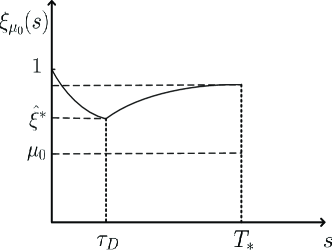
Figure 2: $\mu(s)$ and $\xi_{\mu_{0}}(s)$

Next, we introduce the following lemma to state an important property for UJLC graphs.

Lemma 4.3

If $\mathcal{G}_{\sigma(t)}$ is UJLC, then, for any $t>0$ and $i\in\mathcal{V}_{F}$, there is a path $\widehat{(j,i)}$ from some leader $j\in\mathcal{V}_{L}$ to follower $i$ in $\mathcal{G}([t,t+T_{0}))$ with $T_{0}\triangleq T+2\tau_{D}$, and each arc of $\widehat{(j,i)}$ exists in a time interval with length $\tau_{D}$ at least during $[t,t+T_{0})$.

Proof: Denote $t_{1}$ as the first moment when the interaction topology switches within $[t,t+T_{0})$ (suppose there are switchings without loss of generality). If $t_{1}\geq t+\tau_{D}$, then, for any $i\in\mathcal{V}_{F}$, there is a path $\widehat{(j,i)}$ from some leader with index $j\in\mathcal{V}_{L}$ to agent $i$ in $\mathcal{G}([t,t+T))$, where each arc stays there for at least the dwell time $\tau_{D}$ during $[t,t+T+\tau_{D})$ due to the definition of $\tau_{D}$. On the other hand, if $t_{1}<t+\tau_{D}$, $t_{1}+T+\tau_{D}<t+T_{0}$. Then, for any $i\in\mathcal{V}_{F}$, there is also a path $\widehat{(j,i)}$ from some leader $j\in\mathcal{V}_{L}$ to agent $i$ in $\mathcal{G}([t_{1},t_{1}+T))$ in $[t_{1},t_{1}+T+\tau_{D})$ with each arc exists for at least $\tau_{D}$. This completes the proof. $\square$

Remark 4.2

If there is a convex set $\Omega$ such that ${\cal L}(y(t))\in\Omega,\forall t\geq 0$, that is, $\Omega$ is a positively invariant set for the leaders, then $|x(t)|_{\Omega}\leq|x(t)|_{{\cal L}(y(t))}$. By Theorem 4.1, system (6) is SISS with respect to $\Omega$ with $w$ as the input if $\mathcal{G}_{\sigma(t)}$ is UJLC.

Sometimes, the velocities of the moving leaders and uncertainties in agent dynamics (maybe because of the online estimation) may vanish. To be strict, consider the following condition

$$\begin{cases}\lim_{t\rightarrow+\infty}u_{i}(y,t)=0\,\mbox{uniformly for}\ y;\;i=1,\dots,k;\\ \lim_{t\rightarrow+\infty}w_{j}(t)=0,\;j=1,\dots,n.\end{cases}$$ (24)

Clearly, (24) yields that for any $\varepsilon>0$, there is $T_{\varepsilon}>0$ such that $\|z^{T_{\varepsilon}}\|_{\infty}<\varepsilon$, where $z^{T_{\varepsilon}}$ is the truncated part of $z$ defined on $[T_{\varepsilon},+\infty)$. Suppose (24) holds and $\mathcal{G}_{\sigma(t)}$ is UJLC. Based on Theorem 4.1, for any $\varepsilon>0$, there is $T_{\varepsilon}>0$ such that

$$|x(t)|_{\mathcal{L}(y(t))}\leq\beta(|x(T_{\varepsilon})|_{\mathcal{L}(y(T_{\varepsilon}))},t)+\gamma(\varepsilon).$$

Hence, the set tracking for system (6) with respect to set ${\cal L}(y(t))$ is achieved easily. On the other hand, similar to the proof of Theorem 4.1, the necessity of the global set tracking for system (6) with condition (24) can also be simply proved by counterexamples since $|z(t)|$ may be large and the distance error may accumulate to a very large value over a sufficiently long period of time. Therefore, we have the following result.

Corollary 4.1

The global set tracking with respect to ${\cal L}(y(t))$ is achieved for all $z(t)$ satisfying (24) if and only if $\mathcal{G}_{\sigma(t)}$ is UJLC.

4.2 Proof of Theorem 4.1

We are now in a position to prove Theorem 4.1: “If” part: Denote $T_{\ast}=nT_{0}$ with $T_{0}=T+2\tau_{D}$. Then we estimate $\Psi(t)$ at subintervals $[t^{\ast}+(j-1)T_{0},t^{\ast}+jT_{0}]$ for $j=1,\dots,n$.

Based on Lemma 4.3, in $[t^{\ast},t^{\ast}+T_{0})$, there must be an arc $({j_{1}},{i_{1}})\in\mathcal{E}([t^{\ast},t^{\ast}+T_{0}))$ leaving from a leader ${j_{1}}\in\mathcal{V}_{L}$ to a follower ${i_{1}}\in\mathcal{V}_{L}$ and this arc remains for at least $\tau_{D}$. Suppose $(j_{1},i_{1})\in\mathcal{E}_{\sigma(t)}$ for $t\in[t_{1},t_{1}+\tau_{D})\subset[t^{\ast},t^{\ast}+T_{0})$. According to Lemma 4.1,

$$|x_{i_{1}}(t)|_{\mathcal{L}(y(t))}\leq\mu(t-t_{1})|x(t_{1})|_{\mathcal{L}(y(t_{1}))}+\gamma_{1}\|z\|_{\infty},\;t\in[t_{1},t_{1}+T_{\ast}],$$ (25)

where $\mu(s)$ and $\gamma_{1}$ were defined in Lemma 4.1. Take $\eta_{1}=\sup\limits\{\mu(s)\mid s\in[T_{0},T_{\ast}]\}=\mu(T_{\ast})$. Since $0<\mu_{1}<1$,

$$|x_{i_{1}}(t)|_{\mathcal{L}(y(t))}\leq\eta_{1}|x(t_{1})|_{\mathcal{L}(y(t_{1}))}+\gamma_{1}\|z\|_{\infty},\;t\in[t^{\ast}+T_{0},t^{\ast}+T_{\ast}].$$ (26)

Furthermore, in $[t^{\ast}+T_{0},t^{\ast}+2T_{0})$, there must be a follower ${i_{2}}\in\mathcal{V}_{F},{i_{2}}\neq i_{1}$, such that there exists an arc $({j_{2}},{i_{2}})$ for some ${j_{2}}\in\mathcal{V}_{L}$, or an arc $({i_{1}},{i_{2}})$ in $\mathcal{E}([t^{\ast}+T_{0},t^{\ast}+2T_{0}))$.

There are two cases:

• If $({j_{2}},{i_{2}})\in\mathcal{E}_{\sigma(t)}$ for $t\in[t_{2},t_{2}+\tau_{D})\subset[t^{\ast}+T_{0},t^{\ast}+2T_{0})$, one also has

  $$|x_{i_{2}}(t)|_{\mathcal{L}(y(t))}\leq\eta_{1}|x(t_{2})|_{\mathcal{L}(y(t_{2}))}+\gamma_{1}\|z\|_{\infty},\;t\in[t^{\ast}+2T_{0},t^{\ast}+T_{\ast}].$$ (27)

• If $({i_{1}},{i_{2}})\in\mathcal{E}_{\sigma(t)}$ for $t\in[t_{2},t_{2}+\tau_{D})\subset[t^{\ast}+T_{0},t^{\ast}+2T_{0})$. According to (12) and Lemma 3.2, one has

  $$|x(t_{1})|_{\mathcal{L}(y(t_{1}))}\leq|x(t_{2})|_{\mathcal{L}(y(t_{2}))}+\sqrt{2}\|z\|_{\infty}\cdot|t_{2}-t_{1}|\leq|x(t_{2})|_{\mathcal{L}(y(t_{2}))}+2\sqrt{2}\|z\|_{\infty}T_{0},$$

  Thus, (26) will lead to

  $$|x_{i_{1}}(t)|_{\mathcal{L}(y(t))}\leq\eta_{1}|x(t_{2})|_{\mathcal{L}(y(t_{2}))}+(2\sqrt{2}\eta_{1}T_{0}+\gamma_{1})\|z\|_{\infty},\;t\in[t^{\ast}+T_{0},t^{\ast}+T_{\ast}].$$ (28)

  Then, by Lemma 4.2, if we take $\eta_{2}=\xi_{\eta_{1}}((n-1)T_{0})$, then

  $$|x_{i_{2}}(t)|_{\mathcal{L}(y(t))}\leq\eta_{2}|x(t_{2})|_{\mathcal{L}(y(t_{2}))}+(\gamma_{2}+2\sqrt{2}\eta_{1}T_{0}+\gamma_{1})\|z\|_{\infty},\;t\in[t^{\ast}+2T_{0},t^{\ast}+T_{\ast}].$$ (29)

Because $\eta_{2}>\eta_{1}$,

$$|x_{\jmath}(t)|_{\mathcal{L}(y(t))}\leq\eta_{2}|x(t_{2})|_{\mathcal{L}(y(t_{2}))}+(\gamma_{2}+2\sqrt{2}\eta_{1}T_{0}+\gamma_{1})\|z\|_{\infty},\;\jmath=i_{1},i_{2},t\in[t^{\ast}+2T_{0},t^{\ast}+T_{\ast}].$$ (30)

Repeating the above procedure yields

$$\eta_{j}=\xi_{\eta_{j-1}}((n-j+1)T_{0}),\;j=3,\dots,n$$

and $t_{j}\in[t^{\ast}+jT_{0},t^{\ast}+T_{\ast})$ such that, there exists ${i_{j}}\in\mathcal{V}_{F},\;j=3,\dots,n$ satisfying

$$|x_{\jmath}(t)|_{\mathcal{L}(y(t))}\leq\eta_{j}|x(t_{j})|_{\mathcal{L}(y(t_{j}))}+[(j-1)\gamma_{2}+2\sqrt{2}\sum_{l=1}^{j-1}\eta_{l}T_{0}+\gamma_{1}]\|z\|_{\infty},\;\jmath=i_{1},\dots,i_{j}$$ (31)

for $t\in[t^{\ast}+jT_{0},t^{\ast}+T_{\ast}]$. Moreover, the nodes $i_{j},j=1,2,\dots,n$ are distinct.

Denote $\eta_{\ast}=\eta_{n}$, and then $0<\eta_{\ast}<1$. Thus, (31) leads to

$$|x_{\jmath}(t^{\ast}+T_{\ast})|_{\mathcal{L}(y(t^{\ast}+T_{\ast}))}\leq\eta_{\ast}|x(t^{\ast})|_{\mathcal{L}(y(t^{\ast}))}+[(1+2\sqrt{2})\eta_{\ast}T_{\ast}+(n-1)\gamma_{2}+\gamma_{1}]\|z\|_{\infty},$$ (32)

for any $\jmath\in\mathcal{V}_{F}$, which leads to

$$|x(t^{\ast}+T_{\ast})|_{\mathcal{L}(y(t^{\ast}+T_{\ast}))}\leq\eta_{\ast}|x(t^{\ast})|_{\mathcal{L}(y(t^{\ast}))}+[(1+2\sqrt{2})\eta_{\ast}T_{\ast}+(n-1)\gamma_{2}+\gamma_{1}]\|z\|_{\infty}.$$ (33)

Therefore, $\forall N=1,2,\dots$,

$$|x(NT_{\ast})|_{\mathcal{L}(y(NT_{\ast}))}\leq\eta_{\ast}^{N}|x^{0}|_{\mathcal{L}(y^{0})}+\sum_{j=0}^{N-1}\eta_{\ast}^{j}[(1+2\sqrt{2})\eta_{\ast}T_{\ast}+(n-1)\gamma_{2}+\gamma_{1}]\|z\|_{\infty}.$$ (34)

Again by Lemma 3.2, one has

$$|x(t)|_{\mathcal{L}(y(t))}\leq\beta(|x^{0}|_{\mathcal{L}(y^{0})},t)+\gamma(\|z\|_{\infty})$$ (35)

with

$$\beta(|x^{0}|_{\mathcal{L}(y^{0})},t)\triangleq\eta_{\ast}^{\lfloor\frac{t}{T^{\ast}}\rfloor}|x^{0}|_{\mathcal{L}(y^{0})},\quad\gamma(s)\triangleq[\frac{(1+2\sqrt{2})\eta_{\ast}T_{\ast}+(n-1)\gamma_{2}+\gamma_{1}}{1-\eta_{\ast}}+T_{\ast}]s$$

where $\lfloor\frac{t}{T^{\ast}}\rfloor$ denotes the largest integer no greater than $\frac{t}{T^{\ast}}$, which implies the conclusion.

“Only if” part: If $\mathcal{G}_{\sigma(t)}$ is not UJLC, there is a time sequence $0<T_{1}<T_{2}<\dots$ such that $\mathcal{G}([T_{2\kappa-1},T_{2\kappa}))$ is not L-connected for $\kappa=1,2,\dots$ with $\lim_{\kappa\rightarrow\infty}(T_{2\kappa}-T_{2\kappa-1})=\infty$. Taking $x_{i}(0)=(0,\dots,0)^{T}\in R^{d},\forall i\in\mathcal{V}_{F}$ and $y_{i}(0)=(1,\dots,1)^{T}\in R^{d},\forall i\in\mathcal{V}_{L}$ with $w_{i}(t)\equiv 0,\forall i\in\mathcal{V}_{F}$ and $u_{i}(y,t)\equiv(1,\dots,1)^{T},\forall i\in\mathcal{V}_{L}$, we obtain $\mathcal{L}(y(t))=\{(1+t,\dots,1+t)^{T}\}$. Since $\mathcal{G}([T_{2\kappa-1},T_{2\kappa}))$ is not L-connected, there is $i\in\mathcal{V}_{F}$ such that agent $i$ is reachable from no leader. Define $\hat{\mathcal{V}}_{i}^{1}\triangleq\{j\in\mathcal{V}|i\;\mbox{is reachable from}\;j\ \mbox{in graph}\ \mathcal{G}([T_{2\kappa-1},T_{2\kappa}))\}$. Since $\hat{\mathcal{V}}_{i}^{1}$ contains no leader and there is no arc entering $\hat{\mathcal{V}}_{i}^{1}$, no agent in $\hat{\mathcal{V}}_{i}^{1}$ leaves $co\{x_{\jmath}(T_{2\kappa-1}),\jmath\in\hat{\mathcal{V}}_{i}^{1}\}$ when $t\in[T_{2\kappa-1},T_{2\kappa})$. Moreover, none of the followers can enter $\mathcal{L}(y(t))$ in finite time. Therefore,

$$\lim_{\kappa\to\infty}|x_{\jmath}(T_{2\kappa})|_{\mathcal{L}(y(T_{2\kappa}))}\geq\lim_{\kappa\to\infty}(T_{2\kappa}-T_{2\kappa-1})=+\infty,\quad\forall\jmath\in\hat{\mathcal{V}}_{i}^{1}.$$

Thus, the SISS with respect to $\mathcal{L}(y(t))$ cannot be achieved. $\square$

5 Connectivity and SiISS

In this section, we aim at the connectivity requirement to ensure the set integral-input-to-state stability (SiISS) when $\mathcal{G}_{\sigma(t)}$ is jointly L-connected (JLC).

5.1 Main results

Theorem 4.1 showed an equivalent relationship between SISS and UJLC. However, this is not true for SiISS. Here, we propose a couple of theorems about SiISS. The proofs of these conclusions can be found in the following subsection.

First of all, we propose a sufficient condition.

Theorem 5.1

System (6) is SiISS with respect to $\mathcal{L}(y(t))$ if $\mathcal{G}_{\sigma(t)}$ is UJLC.

Remark 5.1

JLC of $\mathcal{G}_{\sigma(t)}$ (i.e., $\mathcal{G}([t,\infty))$ is L-connected for any $t$) is necessary for the SiISS, though it is not sufficient. If $\mathcal{G}([\tilde{T},\infty))$ is not L-connected for some $\tilde{T}>0$, there is a subset $\hat{\mathcal{V}}_{F}\subseteq\mathcal{V}_{F}$ such that no arcs enter $\hat{\mathcal{V}}_{F}$ in $\mathcal{G}([\tilde{T},\infty))$. Hence, the agents in $\hat{\mathcal{V}}_{F}$ may not be SiISS for some initial conditions since they will not be influenced by the convex leader-set after $\tilde{T}$.

UJLC, which is a special case of JLC, provides a sufficient condition for SiISS, but UJLC is not necessary to ensure SiISS. In fact, there are other cases of JLC to make SiISS hold. Here we consider two important special JLC cases i.e., bidirectional graphs and acyclic graphs.

A digraph $\mathcal{G}$ is called a bidirectional graph when $i$ is a neighbor of $j$ if and only if $j$ is a neighbor of $i$, but the weight of arc $(i,j)$ may not be equal to that of arc $(j,i)$. The next result shows a necessary and sufficient condition for the bidirectional case.

Theorem 5.2

Suppose that $\mathcal{G}^{F}_{\sigma(t)}$ is bidirectional for all $t\geq 0$. Then system (6) is SiISS if and only if $\mathcal{G}_{\sigma(t)}$ is JLC.

The next lemma shows an important property for an acyclic digraph, that is, a digraph without cycles.

Lemma 5.1

Assume that $\mathcal{G}^{F}([0,+\infty))$ is acyclic and $\mathcal{G}([0,+\infty))$ is L-connected. Then there is a partition of $\mathcal{V}_{F}$ by $\mathcal{V}_{F}=\bigcup_{i=1}^{k_{0}}\mathcal{V}_{i}^{F},k_{0}\geq 1$ such that in graph $\mathcal{G}([0,+\infty))$, all the arcs entering node set $\mathcal{V}_{1}^{F}$ are from $\mathcal{V}_{L}$ ; and all the arcs entering node set $\mathcal{V}_{j}^{F},j=2,\dots,k_{0}$ are from $\mathcal{V}_{L}\cup(\bigcup_{i=1}^{j-1}\mathcal{V}_{i}^{F})$.

Proof: First we prove $\mathcal{V}^{F}_{1}$ exists by contradiction. If $\mathcal{V}^{F}_{1}$ does not exist, every agent $i,i\in\mathcal{V}_{F}$ has neighbors within $\mathcal{V}_{F}$ in $\mathcal{G}([0,+\infty))$. Denote $\hat{\mathcal{V}}^{F}_{1}\triangleq\{j\in\mathcal{V}_{F}|\mbox{there\ is\ an\ arc\ leaving\ from}\ \mathcal{V}_{L}\ \mbox{entering}\ j\}$. Clearly $\hat{\mathcal{V}}^{F}_{1}\neq\emptyset$. Take $i_{0}\in\hat{\mathcal{V}}^{F}_{1}$. Then, there is $j_{1}\in\mathcal{V}_{F}$ such that $(j_{1},i_{0})\in\mathcal{G}([0,+\infty))$. Moreover, we can associate $j_{1}$ with $i_{1}\in\hat{\mathcal{V}}^{F}_{1}$ ($i_{1}$ cannot be $i_{0}$, of course) such that there is a path $\widehat{(i_{1},j_{1})}$ in $\mathcal{G}([0,\infty))$ ($i_{1}=j_{1}$ if $j_{1}\in\hat{\mathcal{V}}^{F}_{1}$). Hence, a path $\widehat{(i_{1},i_{0})}$ in $\mathcal{G}([0,+\infty))$ is found. Regarding $i_{1}$ as $i_{0}$ and repeating the above procedure yields the existence of $\widehat{(i_{2},i_{1})}$ in $\mathcal{G}([0,+\infty))$ with $i_{2}\in\hat{\mathcal{V}}^{F}_{1}$. In this way, we obtain a path $\widehat{(i_{l+1},i_{l}})$ in $\mathcal{G}([0,+\infty))$ with $i_{l}\in\hat{\mathcal{V}}^{F}_{1},l=2,3,\dots$. Since the nodes in $\hat{\mathcal{V}}^{F}_{1}$ are finite, there has to be $i_{l_{1}}=i_{l_{2}}$ for some $l_{1}>l_{2}\geq 0$, which lead to a directed cycle in $\mathcal{G}([0,+\infty))$. Therefore, there is $\mathcal{V}^{F}_{1}$ to make the conclusion hold.

Next, by replacing $\mathcal{V}_{L}$ with $\mathcal{V}^{F}_{1}\cup\mathcal{V}_{L}$ in $\mathcal{G}([0,\infty))$, with the same analysis we can find $\mathcal{V}^{F}_{2}$ to make the conclusion hold. Repeating this procedure, since the number of all the agents is finite, there will be a constant $k_{0}\geq 1$ such that $\mathcal{V}_{F}=\bigcup_{i=1}^{k_{0}}\mathcal{V}^{F}_{i}$. This completes the proof. $\square$

Then we have a SiISS result for the acyclic graph case.

Theorem 5.3

Assume that $\mathcal{G}^{F}([0,+\infty))$ is acyclic. Then system (6) is SiISS if and only if $\mathcal{G}_{\sigma(t)}$ is JLC.

Furthermore, consider the following inequality

$$\int_{0}^{+\infty}|z(t)|dt<\infty.$$ (36)

It is not hard to obtain the following results based on Theorems 5.1, 5.2, and 5.3. The proofs are omitted for space limitations.

Corollary 5.1

System (6) achieves the set tracking if (36) holds and $\mathcal{G}_{\sigma(t)}$ is UJLC.

Corollary 5.2

Suppose (36) holds with either $\mathcal{G}^{F}_{\sigma(t)}$ being bidirectional for all $t\geq 0$ or $\mathcal{G}^{F}([0,+\infty))$ being acyclic. Then system (6) achieves the global set tracking if and only if $\mathcal{G}_{\sigma(t)}$ is JLC.

Remark 5.2

In general, the condition (24) does not imply and is not implied by the condition (36). In fact, the considered leaders converge to some points with (36), but the leaders can go to infinity with (24). However, if $z(t)$ is uniformly continuous in $[0,+\infty)$ (which can be guaranteed once $\dot{z}(t)$ is bounded for $t\in[0,+\infty)$), (24) will then be implied by (36) according to Barbalat’s Lemma.

Remark 5.3

Corollaries 5.1 and 5.2 are consistent with Proposition 6 in [34], where (36) and integral-ISS together resulted in the state stability. Moreover, the two corollaries are also consistent with Theorems 15 and 17 in [26], respectively, when $z\equiv 0$. However, different from the limit-set-based approach given in [26], the proposed method by virtue of (43) and (50) also provides the estimation of the convergence rate.

Remark 5.4

Theorems 4.1 and 5.1 with Remark 5.1 proved that for system (6), SISS is equivalent to UJLC, which implies SiISS, while JLC is a necessary condition, namely,

$$SISS\Longleftrightarrow UJLC\Longrightarrow SiISS\Longrightarrow JLC.$$

Thus, $SISS\Longrightarrow SiISS,$ which is consistent with Corollary 4 of [34], where ISS implies iISS. Moreover, Theorems 5.2 and 5.3 show that, in either bidirectional or acyclic case,

$$SiISS\Longleftrightarrow JLC.$$

Remark 5.5

As for set tracking (ST), Corollary 4.1 shows that

$$UJLC\Longleftrightarrow ST,\forall\mbox{z(t) satifying}\ (\ref{C2}).$$

Moreover, Corollaries 5.1 and 5.2 show that as long as (36) holds,

$$UJLC\Longrightarrow ST$$

in general directed cases, and

$$\quad JLC\Longleftrightarrow ST$$

in either bidirectional or acyclic case. Usually, SISS goes with (24) and SiISS with (36), consistent with discussions on ISS and iISS [34, 35]. Additionally, it is worth pointing out that the differences between the statements in Corollaries 4.1 and those in 5.1 result from the fact that UJLC is necessary for SISS, but not necessary to SiISS.

Although our results are consistent with the results on conventional ISS or iISS, the analysis methods given in [34, 35] are mainly based on an equivalent ISS-Lyapunov function, which cannot be applied to our cases with a moving set and switching topologies.

5.2 Proofs

To establish the SiISS in the JLC case, we will analyze the impact of the integral of input $z(t)$ in a time interval and estimate the convergence rates during this time interval by “pasting” different time subintervals together within the interval. The following lemmas are given to estimate the convergence rates in different cases.

Lemma 5.2

If there is an arc $(j,i)$ leaving from $j\in\mathcal{V}_{L}$ entering $i\in\mathcal{V}_{F}$ in $\mathcal{G}_{\sigma(t)}$ for $t\in[t_{0},t_{0}+\tau_{D})$, then there exists a strictly decreasing function $\delta(s):[0,\tau_{D}]\mapsto(0,1]$ with $\delta(0)=1$ such that

$$|x_{i}(t)|_{\mathcal{L}(y(t))}\leq\delta(t-t_{0})|x(t_{0})|_{\mathcal{L}(y(t_{0}))}+2\sqrt{2}\int_{t_{0}}^{t_{0}+\tau_{D}}|z(s)|ds,\;t\in[t_{0},t_{0}+\tau_{D}].$$ (37)

Proof: According to Lemma 3.2, $\psi_{j}(t)\leq\sqrt{\Psi(t)}\leq\sqrt{\Psi(t_{0})}+\int_{t_{0}}^{t}\sqrt{2}|z(s)|ds,\;j=1,...,n$ for any $t>t_{0}>0$. Since there is an arc $(j,i)$ with $j\in\mathcal{V}_{L},i\in\mathcal{V}_{F}$ in $\mathcal{G}_{\sigma(t)}$ for $t\in[t_{0},t_{0}+\tau_{D})$,

$$\frac{d}{dt}\psi_{i}(t)\leq-2b_{\ast}\psi_{i}(t)+2\sqrt{2}|z(t)|\sqrt{\psi_{i}(t)}+2\langle x_{i}-\mathcal{P}_{\mathcal{L}(y(t))}(x_{i}),\sum\limits_{j\in N_{i}(\sigma(t))}a_{ij}(x)(x_{j}-x_{i})\rangle.$$

Based on Lemma 2.1, when $t\in[t_{0},t_{0}+\tau_{D})$,

$$\langle x_{i}(t)-\mathcal{P}_{\mathcal{L}(y(t))}(x_{i}(t)),x_{j}(t)-x_{i}(t)\rangle \leq \sqrt{\psi_{i}(t)}(\sqrt{\Psi(t)}-\sqrt{\psi_{i}(t)})$$

$$\leq \sqrt{\psi_{i}(t)}(\sqrt{\Psi(t_{0})}+\int_{t_{0}}^{t}\sqrt{2}|z(s)|ds-\sqrt{\psi_{i}(t)})$$

Therefore,

$$\frac{d}{dt}\psi_{i}(t)\leq-2[b_{\ast}+(n-1)a^{\ast}]\psi_{i}(t)+2[\sqrt{2}|z(t)|+(n-1)a^{\ast}(\sqrt{\Psi(t_{0})}+\int_{t_{0}}^{t}\sqrt{2}|z(s)|ds)]\sqrt{\psi_{i}(t)},$$

or equivalently,

$$\frac{d}{dt}\sqrt{\psi_{i}(t)}\leq-\lambda\sqrt{\psi_{i}(t)}+[\sqrt{2}|z(t)|+(n-1)a^{\ast}(\sqrt{\Psi(t_{0})}+\int_{t_{0}}^{t_{0}+\tau_{D}}\sqrt{2}|z(s)|ds)]$$

where $\lambda\triangleq b_{\ast}+(n-1)a^{\ast}$ for $t\in[t_{0},t_{0}+\tau_{D})$. Thus,

$$\sqrt{\psi_{i}(t)}\leq\delta(t-t_{0})\sqrt{\Psi(t_{0})}+\frac{b_{\ast}+2(n-1)a^{\ast}}{\lambda}\int_{t_{0}}^{t_{0}+\tau_{D}}\sqrt{2}|z(s)|ds,\;\;t\in[t_{0},t_{0}+\tau_{D})$$

with $\delta(s)\triangleq\frac{b_{\ast}e^{-\lambda s}+(n-1)a^{\ast}}{\lambda},\,s\in[0,\tau_{D}]$, which implies the conclusion. $\square$

Lemma 5.3

Suppose there is an edge $(i,m)$ leaving from $i\in\mathcal{V}_{F}$ entering $m\in\mathcal{V}_{F}$ in $\mathcal{G}_{\sigma(t)}$ and $|x_{i}(t)|_{\mathcal{L}(y(t))}\leq\delta_{0}|x(t_{0})|_{\mathcal{L}(y(t_{0}))}+\tilde{c}_{0}$ with constants $\delta_{0}\in(0,1)$ and $\tilde{c}_{0}>0$ when $t\in[t_{0},t_{0}+\tau_{D})$. Then there is a strictly decreasing function $\varphi_{\delta_{0}}(s):[0,\tau_{D}]\mapsto(0,1]$ with $\varphi_{\delta_{0}}(0)=1$ such that

$$|x_{m}(t)|_{\mathcal{L}(y(t))}\leq\varphi_{\delta_{0}}(t-t_{0})|x(t_{0})|_{\mathcal{L}(y(t_{0}))}+\tilde{c}_{0}+2\sqrt{2}\int_{t_{0}}^{t_{0}+\tau_{D}}|z(s)|ds,\;t\in[t_{0},t_{0}+\tau_{D}].$$ (38)

Lemma 5.4

Given a constant $\hat{T}>0$, if there is $t_{1}\geq t_{0}$ with $\|x_{i}(t_{1})\|_{\mathcal{L}(y(t_{1}))}\leq\varepsilon_{0}|x(t_{0})|_{\mathcal{L}(y(t_{0}))}+\hat{c}_{0}$ for constants $\varepsilon_{0}\in(0,1)$ and $\hat{c}_{0}>0$, then there is a strictly increasing function $\phi_{\varepsilon_{0}}(s):[0,\hat{T}]\mapsto[\varepsilon_{0},1)$ with $\phi_{\varepsilon_{0}}(0)=\varepsilon_{0}$ such that

$$|x_{i}(t)|_{\mathcal{L}(y(t))}\leq\phi_{\varepsilon_{0}}(t-t_{1})|x(t_{0})|_{\mathcal{L}(y(t_{0}))}+\hat{c}_{0}+2\sqrt{2}\int_{t_{0}}^{t_{1}+\hat{T}}|z(s)|ds,\;t\in[t_{1},t_{1}+\hat{T}],$$ (39)

where $\phi_{\varepsilon_{0}}(s)=1-e^{-(n-1)a^{\ast}s}(1-\varepsilon_{0})$.

The proofs of Lemmas 5.3 and 5.4 are similar to that of Lemma 5.2, and therefore, omitted.

Lemma 5.5

Suppose $\mathcal{V}_{F}^{1}\subset\mathcal{V}_{F}$ is an nonempty subset. If there are no arcs leaving from ${V}_{F}\setminus\mathcal{V}_{F}^{1}$ entering $\mathcal{V}_{F}^{1}$ in $\mathcal{G}([t_{1},t_{1}+\hat{T}))$ for a given constant $\hat{T}>0$ and $\|x_{i}(t_{1})\|_{\mathcal{L}(y(t_{1}))}\leq\varepsilon_{0}|x(t_{0})|_{\mathcal{L}(y(t_{0}))}+\hat{c}_{0},\;\forall i\in\mathcal{V}_{F}^{1}$ for constants $\varepsilon_{0}\in(0,1)$ and $\hat{c}_{0}>0$, then

$$|x_{i}(t)|_{\mathcal{L}(y(t))}\leq\varepsilon_{0}|x(t_{0})|_{\mathcal{L}(y(t_{0}))}+\hat{c}_{0}+\sqrt{2}\int_{t_{1}}^{t_{1}+t}|z(s)|ds,\quad$$ (40)

Taking $\Psi_{1}(t)=\max\limits_{i\in\mathcal{V}_{F}^{1}}\{\psi_{i}(t)\}$ gives $D^{+}\sqrt{\Psi_{1}(t)}\leq\sqrt{2}|z(t)|$ for $t\in[t_{1},t_{1}+\hat{T}]$ by virtue of the analysis given for Lemma 3.2. Then Lemma 5.5 can be obtained straightforwardly.

Now we are ready to prove Theorems 5.1, 5.2, and 5.3.

Proof of Theorem 5.1: Denote $T_{\ast}=nT_{0}$ with $T_{0}=T+2\tau_{D}$ defined in Lemma 4.3. If $\mathcal{G}([t^{\ast},t^{\ast}+T_{0}))$ is L-connected, there has to be an arc $(j_{1},i_{1})\in\mathcal{E}_{\sigma(t)}$ for $t\in[t_{1},t_{1}+\tau_{D})\subset[t^{\ast},t^{\ast}+T_{0})$ leaving from a leader ${j_{1}}\in\mathcal{V}_{L}$ entering ${i_{1}}\in\mathcal{V}_{L}$ and this arc is kept there for a period of at least $\tau_{D}$. Invoking Lemmas 5.2 and 5.4,

$$|x_{i_{1}}(t)|_{\mathcal{L}(y(t))}\leq c_{1}|x(t_{1})|_{\mathcal{L}(y(t_{1}))}+4\sqrt{2}\int_{t^{\ast}}^{t^{\ast}+T_{\ast}}|z(s)|ds,\;\;t\in[t_{1},t^{\ast}+T_{\ast}],$$

where $c_{1}=\phi_{\delta(\tau_{D})}(T_{\ast})$.

Furthermore, when $t\in[t^{\ast}+T_{0},t^{\ast}+2T_{0})$, there must be a follower ${i_{2}}\in\mathcal{V}_{F},{i_{2}}\neq i_{1}$ such that there exists an arc $({j_{2}},{i_{2}})$ for some ${j_{2}}\in\mathcal{V}_{L}$, or an arc $({i_{1}},{i_{2}})$ when $t\in[t_{2},t_{2}+\tau_{D})\subset[t^{\ast}+T_{0},t^{\ast}+2T_{0}))$. According to Lemmas 5.3 and 5.4,

$$|x_{i_{2}}(t)|_{\mathcal{L}(y(t))}\leq c_{2}|x(t_{1})|_{\mathcal{L}(y(t_{1}))}+8\sqrt{2}\int_{t^{\ast}}^{t^{\ast}+T_{\ast}}|z(s)|ds,\;t\in[t_{2},t^{\ast}+T_{\ast}],$$

where $c_{2}=\phi_{\varphi_{2}}(T_{\ast})$ with $\varphi_{2}=\varphi_{c_{1}}(\tau_{D})$.

Repeating the above procedure yields

$$|x_{i_{\ell}}(t)|_{\mathcal{L}(y(t))}\leq c_{\ell}|x(t_{1})|_{\mathcal{L}(y(t_{1}))}+4\sqrt{2}\ell\int_{t^{\ast}}^{t^{\ast}+T_{*}}|z(s)|ds,\;t\in[t^{\ast}+\ell T_{0},t^{\ast}+T_{\ast}].$$

for ${i_{\ell}}\in\mathcal{V}_{F},\;\ell=3,\dots,n$, where

$$c_{\ell}=\phi_{\varphi_{\ell-1}}(T_{\ast}),\varphi_{\ell}=\varphi_{c_{\ell-1}}(\tau_{D}),[t_{\ell},t_{\ell}+\tau_{D})\subset[t^{\ast}+(\ell-1)T_{0},t^{\ast}+\ell T_{0})$$ (41)

Moreover, the nodes of ${i_{\ell}},\ell=1,2,\dots,n$ are distinct.

Denote $\hat{c}\triangleq c_{n}$ from (41). Then we obtain

$$|x(t^{\ast}+T_{\ast})|_{\mathcal{L}(y(t^{\ast}+T_{\ast}))}\leq\hat{c}|x(t^{\ast})|_{\mathcal{L}(y(t^{\ast}))}+(4n+1)\sqrt{2}\int_{t^{\ast}}^{t^{\ast}+T_{\ast}}|z(s)|ds.$$ (42)

It follows immediately that

$$|x(KT_{\ast})|_{\mathcal{L}(y(KT_{\ast}))}\leq\hat{c}^{K}|x^{0}|_{\mathcal{L}(y^{0})}+(4n+1)\sqrt{2}\sum_{j=1}^{K}\int_{(j-1)T_{\ast}}^{jT_{\ast}}\hat{c}^{K-j}|z(s)|ds,\quad K=1,2,\dots$$ (43)

Based on Lemma 3.2 and (12), we have

$$|x(t)|_{\mathcal{L}(y(t)} \leq \hat{c}^{\lfloor\frac{t}{T^{\ast}}\rfloor}|x^{0}|_{\mathcal{L}(y^{0})}+(4n+1)\sqrt{2}\sum_{j=1}^{\lfloor\frac{t}{T^{\ast}}\rfloor}\int_{(j-1)T_{\ast}}^{jT_{\ast}}\hat{c}^{\lfloor\frac{t}{T^{\ast}}\rfloor-j}|z(s)|ds+\sqrt{2}\int_{\lfloor\frac{t}{T^{\ast}}\rfloor}^{t}|z(s)|ds$$ (44)

$$\leq \hat{c}^{\lfloor\frac{t}{T^{\ast}}\rfloor}|x^{0}|_{\mathcal{L}(y^{0})}+(4n+1)\sqrt{2}\int_{0}^{t}\hat{c}^{\lfloor\frac{t}{T^{\ast}}\rfloor-p(s)}|z(s)|ds$$

where

$$p(s)=\left\{\begin{array}[]{ll}i,\quad\quad s\in[(i-1)T^{\ast},iT^{\ast})\ for\ i=1,\dots,\lfloor\frac{t}{T^{\ast}}\rfloor\\ \lfloor\frac{t}{T^{\ast}}\rfloor,\quad\quad s\in[T^{\ast}\cdot\lfloor\frac{t}{T^{\ast}}\rfloor,t)\end{array}\right.$$ (45)

Hence, (10) holds with $\gamma(s)=(4n+1)\sqrt{2}s$ since $|\hat{c}^{\lfloor\frac{t}{T^{\ast}}\rfloor-p(s)}|\leq 1$, which completes the proof. $\square$

Proof of Theorem 5.2: The “only if” part is quite obvious, so we focus on the “if” part.

Since $\mathcal{G}_{\sigma(t)}$ is JLC, there exists a sequence of time instants

$$0=T_{1}<T_{2}<\dots<T_{i}<T_{i+1}<\dots$$ (46)

such that

$$T_{i}\triangleq T_{i_{1}}<T_{i_{2}}<\dots<T_{i_{n+1}}=T_{i+1},\;i=1,2,\dots$$ (47)

and $\mathcal{G}([T_{i_{\kappa}},T_{i_{\kappa+1}}))$ is L-connected for $\kappa=1,\dots,n$. Moreover, each arc in $\mathcal{G}([T_{i_{k}},T_{i_{k+1}}))$ will be kept for at least the dwell time $\tau_{D}$ during the time interval $[T_{i_{\kappa}},T_{i_{\kappa+1}}),i=1,2,\dots;\kappa=1,2,\dots,n$.

Then we estimate $\Psi(t)$ during $t\in[T_{i},T_{i+1}]$. Since $\mathcal{G}([T_{i_{1}},T_{i_{2}}))$ is L-connected, there is a time interval $[t_{1},t_{1}+\tau_{D})\subseteq[T_{i_{1}},T_{i_{2}})$ such that there is an edge $(l,m_{0})\in\mathcal{E}_{\sigma(t)}$ between a leader $l\in\mathcal{V}_{L}$ and a follower $m_{0}\in\mathcal{V}_{F}$ for $t\in[t_{1},t_{1}+\tau_{D})$. Based on Lemma 5.2,

$$|x_{m_{0}}(t_{1}+\tau_{D})|_{\mathcal{L}(y(t_{1}+\tau_{D}))}\leq\delta_{1}|x(t_{1})|_{\mathcal{L}(y(t_{1}))}+2\sqrt{2}\int_{t_{1}}^{t_{1}+\tau_{D}}|z(s)|ds,$$

where $\delta_{1}\triangleq\delta(\tau_{D})$.

Furthermore, we define $\mathcal{V}_{L}^{1}\triangleq\{v_{m_{0}}\}\cup\mathcal{V}_{L}$,

$$t_{2}\triangleq\inf_{t}\{t\in[t_{1}+\tau_{D},T_{i_{3}})|\mbox{there is an edge leaving from}\ \mathcal{V}_{L}^{1}\ \mbox{entering}\ \mathcal{V}\setminus\mathcal{V}_{L}^{1}\ \mbox{in}\ \mathcal{G}_{\sigma(t)}\},$$

and $\mathcal{V}_{F}^{1}\triangleq\{\jmath\in\mathcal{V}_{F}\setminus m_{0}|\mbox{there is an edge leaving from}\ \mathcal{V}_{L}^{1}\ \mbox{entering}\ \jmath\ \mbox{when}\ t=t_{2}\}.$

Noting that $\mathcal{G}([T_{i_{2}},T_{i_{3}}))$ is L-connected, thus, according to Lemma 5.5, one has

$$|x_{m_{0}}(t_{2})|_{\mathcal{L}(y(t_{2}))}\leq\delta_{1}|x(t_{1})|_{\mathcal{L}(y(t_{1}))}+\sqrt{2}\int_{t_{1}+\tau_{D}}^{t_{2}}|z(s)|ds+2\sqrt{2}\int_{t_{1}}^{t_{1}+\tau_{D}}|z(s)|ds$$

Further, by Lemma 5.4,

$$|x_{m_{0}}(t)|_{\mathcal{L}(y(t))} \leq \phi_{1}|x(t_{1})|_{\mathcal{L}(y(t_{1}))}+\sqrt{2}[2\int_{t_{1}}^{t_{2}+\tau_{D}}+\int_{t_{1}+\tau_{D}}^{t_{2}}+2\int_{t_{1}}^{t_{1}+\tau_{D}}]|z(s)|ds$$ (48)

$$\leq \phi_{1}|x(t_{1})|_{\mathcal{L}(y(t_{1}))}+4\sqrt{2}\int_{t_{1}}^{t_{2}+\tau_{D}}|z(s)|ds$$

for $t\in[t_{2},t_{2}+\tau_{D}]$, where $\phi_{1}\triangleq\phi_{\delta_{1}}(\tau_{D})$. Moreover, according to Lemma 5.3,

$$|x_{\jmath}(t_{2}+\tau_{D})|_{\mathcal{L}(y(t_{2}+\tau_{D}))} \leq \varphi_{\phi_{1}}(\tau_{D})|x(t_{1})|_{\mathcal{L}(y(t_{1}))}+\sqrt{2}[4\int_{t_{1}}^{t_{2}+\tau_{D}}+2\int_{t_{2}}^{t_{2}+\tau_{D}}+2\int_{t_{1}}^{t_{2}}]|z(s)|ds$$ (49)

$$\leq \varphi_{\phi_{1}}(\tau_{D})|x(t_{1})|_{\mathcal{L}(y(t_{1}))}+8\sqrt{2}\int_{t_{1}}^{t_{2}+\tau_{D}}|z(s)|ds$$

for $\jmath\in\mathcal{V}^{1}_{F}$. Because $\phi_{1}<\varphi_{\phi_{1}}(\tau_{D})$, (48) and (49) lead to

$$|x_{i}(t_{2}+\tau_{D})|_{\mathcal{L}(y(t_{2}+\tau_{D}))}\leq\delta_{2}|x(t_{1})|_{\mathcal{L}(y(t_{1}))}+8\sqrt{2}\int_{t_{1}}^{t_{2}+\tau_{D}}|z(s)|ds,\;\forall i\in\{v_{m_{0}}\}\cup\mathcal{V}^{1}_{F},$$

where $\delta_{2}\triangleq\varphi_{\phi_{1}}(\tau_{D})$.

Next, define $\mathcal{V}^{2}_{L}\triangleq\mathcal{V}^{1}_{L}\cup\mathcal{V}^{1}_{F}$,

$$t_{3}\triangleq\inf_{t}\{t\in[t_{2}+\tau_{D},T_{i_{4}})|\mbox{there is an edge leaving from}\ \mathcal{V}^{2}_{L}\ \mbox{and entering}\ \mathcal{V}\setminus\mathcal{V}_{L}^{2}\ \mbox{in}\ \mathcal{G}_{\sigma(t)}\}$$

and $\mathcal{V}^{2}_{F}\triangleq\{\jmath\in\mathcal{V}\setminus\mathcal{V}_{L}^{2}|\mbox{there is an edge leaving from}\ \mathcal{V}^{2}_{L}\ \mbox{entering}\ \jmath\ \mbox{when}\ t=t_{3}\}.$

Similarly, from Lemma 5.5, by $\phi_{2}\triangleq\phi_{\delta_{2}}(\tau_{D}),\;\delta_{3}\triangleq\varphi_{\phi_{2}}(\tau_{D}),$ one has

$$|x_{i}(t_{3}+\tau_{D})|_{\mathcal{L}(y(t_{3}+\tau_{D}))}\leq\delta_{3}|x(t_{1})|_{\mathcal{L}(y(t_{1}))}+12\sqrt{2}\int_{t_{1}}^{t_{3}+\tau_{D}}|z(s)|ds,\quad\forall i\in\{v_{m_{0}}\}\cup\mathcal{V}^{1}_{F}\cup\mathcal{V}^{2}_{F}$$

Repeating the process gives

$$\phi_{\kappa}\triangleq\phi_{\delta_{\kappa}}(\tau_{D}),\quad\delta_{\kappa+1}\triangleq\varphi_{\phi_{\kappa}}(\tau_{D}),$$

for $\kappa=3,4,\dots,k_{0}$ until $\mathcal{V}_{F}=\{v_{m_{0}}\}\cup\mathcal{V}^{1}_{F}\cup\mathcal{V}^{2}_{F}\cup\dots\cup\mathcal{V}^{k_{0}}_{F}$ for some $k_{0}\leq n$ such that

$$|x_{i}(t_{k_{0}}+\tau_{D})|_{\mathcal{L}(y(t_{k_{0}}+\tau_{D}))}\leq\delta_{k_{0}}|x(t_{1})|_{\mathcal{L}(y(t_{1}))}+4\sqrt{2}k_{0}\int_{t_{1}}^{t_{k_{0}}+\tau_{D}}|z(s)|ds,\quad\forall i\in\mathcal{V}_{F}$$

Hence

$$|x(t_{k_{0}}+\tau_{D})|_{\mathcal{L}(y(t_{k_{0}}+\tau_{D}))}\leq\delta_{k_{0}}|x(t_{1})|_{\mathcal{L}(y(t_{1}))}+4\sqrt{2}k_{0}\int_{t_{1}}^{t_{k_{0}}+\tau_{D}}|z(s)|ds$$

According to Lemma 5.5, we obtain

$$|x(T_{i+1})|_{\mathcal{L}(y(T_{i+1}))}\leq\delta_{k_{0}}|x(T_{i})|_{\mathcal{L}(y(T_{i}))}+(4k_{0}+1)\sqrt{2}\int_{T_{i}}^{T_{i+1}}|z(s)|ds.$$

It is obvious to see that $k_{0}\leq n$ and $0<\delta_{1}\leq\delta_{2}\leq\dots\delta_{n}<1$. Therefore, denote $\hat{\delta}\triangleq\delta_{n}$, then for $K=1,2,\dots$,

$$|x(T_{K+1})|_{\mathcal{L}(y(T_{K+1}))}\leq\hat{\delta}^{K}|x^{0}|_{\mathcal{L}(y^{0})}+(4n+1)\sqrt{2}\sum_{i=1}^{K}\hat{\delta}^{K-i}\int_{T_{i}}^{T_{i+1}}|z(s)|ds$$ (50)

Thus, similar to the proof of Theorem 5.1, we also have

$$|x(t)|_{\mathcal{L}(y(t)}\leq\hat{\delta}^{\Gamma(t)}|x^{0}|_{\mathcal{L}(y^{0})}+(4n+1)\sqrt{2}\int_{0}^{t}\hat{\delta}^{\Gamma(t)-\hat{p}(s)}|z(s)|ds$$ (51)

where $\Gamma(t)=K_{0}-1$ when $t\in[T_{K_{0}},T_{K_{0}+1}),K_{0}=1,2,\dots$, and

$$\hat{p}(s)=\left\{\begin{array}[]{ll}i,\quad\quad s\in[T_{i},T_{i+1})\ for\ i=1,\dots,K_{0}-1\\ K_{0}-1,\quad\quad s\in[T_{K_{0}},t)\end{array}\right.$$ (52)

Then it is obvious to see that (51) leads to Theorem 5.2 immediately. $\square$

Proof of Theorem 5.3: We also focus on the “if” part since the “only if” part is quite obvious.

Because $\mathcal{G}_{\sigma(t)}$ is JLC, there is an infinite sequence in the form of (46) with (47) such that $\mathcal{G}([T_{i_{\kappa}},T_{i_{\kappa+1}}))$ is L-connected for $\kappa=1,\dots,n$.

Then, for any $\ell\in\mathcal{V}_{1}$, there is $t_{\ell}\in[T_{i_{1}},T_{i_{2}})$ such that there is an arc leaving from $\mathcal{V}_{F}$ entering $\ell$ in $\mathcal{G}_{\sigma(t)}$. Hence, recalling Lemma 5.2,

$$|x_{\ell}(t_{\ell}+\tau_{D})|_{\mathcal{L}(y(t_{\ell}+\tau_{D}))}\leq d_{1}|x(t_{\ell})|_{\mathcal{L}(y(t_{\ell}))}+2\sqrt{2}\int_{t_{\ell}}^{t_{\ell}+\tau_{D}}|z(s)|ds,\;\ell\in\mathcal{V}_{1}^{F}$$

with a constant $d_{1}\triangleq\delta(\tau_{D})$. According to Lemma 5.1, for any $\ell\in\mathcal{V}_{1}^{F}$, we have

$$|x_{\ell}(t)|_{\mathcal{L}(y(t))}\leq d_{1}|x(T_{i})|_{\mathcal{L}(y(T_{i}))}+2\sqrt{2}\int_{T_{i}}^{T_{i+1}}|z(s)|ds,\;t\in[T_{i_{2}},T_{i+1}]$$

Again by Lemmas 5.3 and 5.1, for any $\ell\in\mathcal{V}_{2}^{F}$,

$$|x_{\ell}(t)|_{\mathcal{L}(y(t))}\leq d_{2}|x(T_{i})|_{\mathcal{L}(y(T_{i}))}+4\sqrt{2}\int_{T_{i}}^{T_{i+1}}|z(s)|ds,\;t\in[T_{i_{3}},T_{i+1}],$$

where $d_{2}=\varphi_{d_{1}}(\tau_{D})$. Similarly, with $d_{j}=\varphi_{d_{j-1}}(\tau_{D}),j=3,\dots,k_{0}$,

$$|x_{\ell}(t)|_{\mathcal{L}(y(t))}\leq d_{j}|x(T_{i})|_{\mathcal{L}(y(T_{i}))}+2\sqrt{2}j\int_{T_{i}}^{T_{i+1}}|z(s)|ds,\;t\in[T_{i_{j+1}},T_{i+1}],$$

for any $\ell\in\mathcal{V}_{j}^{F},j=3,\dots,k_{0}$, which leads to

$$|x(T_{i+1})|_{\mathcal{L}(y(T_{i+1}))}\leq d_{k_{0}}|x(T_{i})|_{\mathcal{L}(y(T_{i}))}+2\sqrt{2}k_{0}\int_{T_{i}}^{T_{i+1}}|z(s)|ds.$$

Similar to the proof of Theorem 5.2, SiISS can be obtained. $\square$

6 Conclusions

This paper addressed multi-agent set tracking problems with multiple leaders and switching communication topologies. At first, the equivalence between UJLC and the SISS of a group of uncertain agents with respect to a moving multi-leader set was shown. Then it was shown that UJLC is a sufficient condition for SiISS of the multi-agent system with disturbances in agent dynamics and unmeasurable velocities in the dynamics of the leaders. Moreover, when communication topologies are either bidirectional or acyclic, JLC is a necessary and sufficient condition for SiISS. Also, set tracking was achieved in special cases with the help of SISS and SiISS.

Multiple leaders, in some practical cases, can provide an effective way to overcome the difficulties and constraints in the distributed design. On the other hand, ISS-based tools were proved to be very powerful in the control synthesis. Therefore, the study of multiple active leaders and related ISS tools deserves more attention.

Appendix

A.1   Proof of Lemma 4.1

Due to $D^{+}\sqrt{\Psi(t)}\leq\sqrt{2}\|z\|_{\infty}$ by Lemma 3.2 and (12), we obtain

$$\sqrt{\psi_{j}(t)}\leq\sqrt{\Psi(t)}\leq\sqrt{\Psi(t_{0})}+\sqrt{2}\|z\|_{\infty}(t-t_{0}),\;j=1,...,n.$$ (53)

Since there is an arc $(j,i)$ with $j\in\mathcal{V}_{L}$ and $i\in\mathcal{V}_{F}$ in $\mathcal{G}_{\sigma(t)}$ for $t\in[t_{0},t_{0}+\tau_{D})$, based on (20), one has

$$\langle x_{i}-\mathcal{P}_{\mathcal{L}(y(t))}(x_{i}),\sum_{j\in L_{i}(\sigma(t))}b_{ij}(x)(y_{j}-x_{i})\rangle\leq-b_{\ast}\psi_{i}(t).$$ (54)

Thus, with (19) and the fact that $r(t)+w_{i}(t)\leq q(t)\leq\sqrt{2}\|z\|_{\infty}$, we obtain

$$\frac{d}{dt}\psi_{i}(t) \leq -2b_{\ast}\psi_{i}(t)+2\langle x_{i}-\mathcal{P}_{\mathcal{L}(y(t))}(x_{i}),\sum\limits_{j\in N_{i}(\sigma(t))}a_{ij}(x_{j}-x_{i})\rangle+2(r(t)+w_{i}(t))\sqrt{\psi_{i}(t)}$$ (55)

$$\leq -2b_{\ast}\psi_{i}(t)+2\langle x_{i}-\mathcal{P}_{\mathcal{L}(y(t))}(x_{i}),\sum\limits_{j\in N_{i}(\sigma(t))}a_{ij}(x_{j}-x_{i})\rangle+2\sqrt{2}\|z\|_{\infty}\sqrt{\psi_{i}(t)}$$

for $t\in[t_{0},t_{0}+\tau_{D})$.

Then, by Lemma 2.1, if $\sqrt{\psi_{j}(t)}<\sqrt{\psi_{i}(t)},j\in N_{i}(\sigma(t))$ for $t\in[t_{0},t_{0}+\tau_{D})$, then

$$\langle x_{i}(t)-\mathcal{P}_{\mathcal{L}(y(t))}(x_{i}(t)),x_{j}(t)-x_{i}(t)\rangle\leq 0.$$ (56)

On the other hand, if $\sqrt{\psi_{j}(t)}\geq\sqrt{\psi_{i}(t)},j\in N_{i}(\sigma(t))$, from Lemma 2.1 and (53),

$$\langle x_{i}(t)-\mathcal{P}_{\mathcal{L}(y(t))}(x_{i}(t)),x_{j}(t)-x_{i}(t)\rangle \leq \sqrt{\psi_{i}(t)}(\sqrt{\psi_{j}(t)}-\sqrt{\psi_{i}(t)})$$ (57)

$$\leq \sqrt{\psi_{i}(t)}(\sqrt{\Psi(t_{0})}+\sqrt{2}\|z\|_{\infty}(t-t_{0})-\sqrt{\psi_{i}(t)})$$

$$\leq \sqrt{\psi_{i}(t)}(\sqrt{\Psi(t_{0})}-\sqrt{\psi_{i}(t)}+\sqrt{2}\|z\|_{\infty}\tau_{D})$$

$t\in[t_{0},t_{0}+\tau_{D})$. Therefore, with (55), (56) and (57), it follows that

$$\frac{d}{dt}\psi_{i}(t)\leq-2\lambda\psi_{i}(t)+2[\sqrt{2}\|z\|_{\infty}(1+(n-1)a^{\ast}\tau_{D})+(n-1)a^{\ast}\sqrt{\Psi(t_{0})}]\sqrt{\psi_{i}(t)},$$

where $\lambda\triangleq b_{\ast}+(n-1)a^{\ast}$, or equivalently,

$$\frac{d}{dt}\sqrt{\psi_{i}(t)}\leq-\lambda\sqrt{\psi_{i}(t)}+[\sqrt{2}\|z\|_{\infty}(1+(n-1)a^{\ast}\tau_{D})+(n-1)a^{\ast}\sqrt{\Psi(t_{0})})]$$

for $t\in[t_{0},t_{0}+\tau_{D})$. As a result,

$$\sqrt{\psi_{i}(t)} \leq e^{-\lambda(t-t_{0})}\sqrt{\Psi(t_{0})}+(1-e^{-\lambda(t-t_{0})})\frac{(n-1)a^{\ast}\sqrt{\Psi(t_{0})}+(\|u\|_{\infty}+\|w\|_{\infty})(1+(n-1)a^{\ast}\tau_{D})}{\lambda}$$ (58)

$$\leq \hat{\mu}(t-t_{0})\sqrt{\Psi(t_{0})}+c_{0}\sqrt{2}\|z\|_{\infty},\qquad\qquad t\in[t_{0},t_{0}+\tau_{D})$$

where $\hat{\mu}(s)\triangleq\frac{b_{\ast}e^{-\lambda s}+(n-1)a^{\ast}}{b_{\ast}+(n-1)a^{\ast}},\,s\in[0,\tau_{D}]$ and $c_{0}\triangleq\frac{1+(n-1)a^{\ast}\tau_{D}}{b_{\ast}+(n-1)a^{\ast}}$, because $1-e^{-\lambda(t-t_{0})}<1$.

Then we evaluate $\sqrt{\psi_{i}(t)}$ for $t\in[t_{0}+\tau_{D},t_{0}+T_{\ast})$ no matter whether there is any connection between the followers and the leaders. Similar analysis gives

$$\frac{d}{dt}\psi_{i}(t) \leq 2\sqrt{2}\|z\|_{\infty}\sqrt{\psi_{i}(t)}+2\langle x_{i}-\mathcal{P}_{\mathcal{L}(y(t))}(x_{i}),\sum\limits_{j\in N_{i}(\sigma(t))}a_{ij}(x)(x_{j}-x_{i})\rangle$$

$$\leq 2\sqrt{2}\|z\|_{\infty}\sqrt{\psi_{i}(t)}+2(n-1)a^{\ast}\sqrt{\psi_{i}(t)}(\sqrt{\Psi(t_{0})}-\sqrt{\psi_{i}(t)}+\sqrt{2}\|z\|_{\infty}T_{\ast})$$

$$= -2(n-1)a^{\ast}\psi_{i}(t)+2[\sqrt{2}\|z\|_{\infty}(1+(n-1)a^{\ast}T_{\ast})+(n-1)a^{\ast}\sqrt{\Psi(t_{0})}]\sqrt{\psi_{i}(t)},$$

which is equivalent to

$$\frac{d}{dt}\sqrt{\psi_{i}(t)}\leq-(n-1)a^{\ast}\sqrt{\psi_{i}(t)}+[\sqrt{2}\|z\|_{\infty}(1+(n-1)a^{\ast}T_{\ast})+(n-1)a^{\ast}\sqrt{\Psi(t_{0})}].$$ (59)

Denote $\hat{\mu}^{\ast}\triangleq\hat{\mu}(\tau_{D})$. From (58), when $t\in[t_{0}+\tau_{D},t_{0}+T_{\ast})$,

$$\sqrt{\psi_{i}(t)} \leq e^{-(n-1)a^{\ast}(t-(t_{0}+\tau_{D}))}\sqrt{\psi_{i}(t_{0}+\tau_{D})}$$ (60)

$$+(1-e^{-(n-1)a^{\ast}(t-(t_{0}+\tau_{D}))})[\sqrt{\Psi(t_{0})}+\sqrt{2}\|z\|_{\infty}\frac{1+(n-1)a^{\ast}T_{\ast}}{(n-1)a^{\ast}}]$$

$$\leq e^{-(n-1)a^{\ast}(t-(t_{0}+\tau_{D}))}[\hat{\mu}^{\ast}\sqrt{\Psi(t_{0})}+c_{0}\sqrt{2}\|z\|_{\infty}]$$

$$+(1-e^{-(n-1)a^{\ast}(t-(t_{0}+\tau_{D}))})[\sqrt{\Psi(t_{0})}+\sqrt{2}\|z\|_{\infty}\cdot\frac{1+(n-1)a^{\ast}T_{\ast}}{(n-1)a^{\ast}}]$$

$$\leq \tilde{\mu}(t-t_{0})\sqrt{\Psi(t_{0})}+\gamma_{1}\|z\|_{\infty},$$

where $\gamma_{1}\triangleq\sqrt{2}\cdot\frac{1+(n-1)a^{\ast}T_{\ast}}{(n-1)a^{\ast}}>c_{0}$ and $\tilde{\mu}(s)\triangleq 1-e^{-(n-1)a^{\ast}(s-\tau_{D}))}(1-\hat{\mu}^{\ast}),s\in[\tau_{D},T_{\ast}]$. Therefore, based on (58) and (60),

$$\sqrt{\psi_{i}(t)}\leq\mu(t-t_{0})\sqrt{\Psi(t_{0})}+\gamma_{1}\|z\|_{\infty},\quad\mu(s)=\left\{\begin{array}[]{ll}\hat{\mu}(s),&\mbox{$s\in[0,\tau_{D})$}\\ \tilde{\mu}(s),&\mbox{$s\in[\tau_{D},T_{\ast}]$}\end{array}\right.$$

where $\mu(s)$ is continuous. Thus, the conclusion follows. $\square$

A.2  Proof of Lemma 4.2

If there is an arc $(v_{i},v_{m})$ in $\mathcal{G}_{\sigma(t)}$ for $t\in[t_{0},t_{0}+\tau_{D})$, then based on (53), Lemmas 2.1 and 3.1, it is easy to see

$$\frac{d}{dt}\psi_{m}(t) \leq 2\langle x_{m}-\mathcal{P}_{\mathcal{L}(y(t))}(x_{m}),\sum\limits_{j\in N_{m}(\sigma(t))}a_{mj}(x)(x_{j}-x_{m})+\sum_{j\in L_{m}(\sigma(t))}b_{mj}(x)(y_{j}-x_{m})\rangle$$

$$+2\sqrt{2}\|z\|_{\infty}\sqrt{\psi_{m}(t)}$$

$$\leq 2\sqrt{2}\|z\|_{\infty}\sqrt{\psi_{m}(t)}+2\langle x_{m}-\mathcal{P}_{\mathcal{L}(y(t))}(x_{m}),\sum\limits_{j\in N_{m}(\sigma(t))}a_{mj}(x)(x_{j}-x_{m})\rangle$$

$$= 2\sqrt{2}\|z\|_{\infty}\sqrt{\psi_{m}(t)}+2\sum\limits_{j\in N_{m}(\sigma(t))\setminus v_{i}}a_{mj}(x)\langle x_{m}-\mathcal{P}_{\mathcal{L}(y(t))}(x_{m}),x_{j}-x_{m}\rangle$$

$$+2a_{mi}(x)\langle x_{m}-\mathcal{P}_{\mathcal{L}(y(t))}(x_{m}),x_{i}-x_{m}\rangle$$

$$\leq 2\sqrt{2}\|z\|_{\infty}\sqrt{\psi_{m}(t)}+2(n-2)a^{\ast}\sqrt{\psi_{m}(t)}(\sqrt{\Psi(t_{0})}-\sqrt{\psi_{m}(t)}+\sqrt{2}\|z\|_{\infty}\tau_{D})$$

$$-2a_{\ast}\sqrt{\psi_{m}(t)}(\sqrt{\psi_{m}(t)}-\sqrt{\psi_{i}(t)})$$

for $t\in[t_{0},t_{0}+\tau_{D})$. Then, if (22) holds, as done in the proof of Lemma 4.1, we can obtain

$$\frac{d}{dt}\sqrt{\psi_{m}(t)}\leq-\lambda_{1}\sqrt{\psi_{m}(t)}+\hat{d}_{1}$$

where $\lambda_{1}\triangleq(n-2)a^{\ast}+a_{\ast}$ and $\hat{d}_{1}\triangleq(1+(n-2)a^{\ast}\tau_{D})\sqrt{2}\|z\|_{\infty}+((n-2)a^{\ast}+a_{\ast}\mu_{0})\sqrt{\Psi(t_{0})}+a_{\ast}d_{0}$. Here are two cases.

• when $t\in[t_{0},t_{0}+\tau_{D})$:

  $$\sqrt{\psi_{m}(t)} \leq e^{-\lambda_{1}(t-t_{0})}\sqrt{\psi_{m}(t_{0})}+(1-e^{-\lambda_{1}(t-t_{0})})\frac{\hat{d}_{1}}{\lambda_{1}}$$ (61)

  $$\leq \frac{(n-2)a^{\ast}+(\mu_{0}+(1-\mu_{0})e^{-\lambda_{1}(t-t_{0})})a_{\ast}}{(n-2)a^{\ast}+a_{\ast}}\sqrt{\Psi(t_{0})}+(1-e^{-\lambda_{1}(t-t_{0})})$$

  $$\cdot\frac{\sqrt{2}\|z\|_{\infty}(1+(n-2)a^{\ast}\tau_{D})+a_{\ast}d_{0}}{(n-2)a^{\ast}+a_{\ast}}$$

  $$\leq \hat{\xi}(t-t_{0})\sqrt{\Psi(t_{0})}+\gamma_{0},$$

  where $\hat{\xi}(s)\triangleq\frac{(n-2)a^{\ast}+(\mu_{0}+(1-\mu_{0})e^{-\lambda_{1}s})a_{\ast}}{(n-2)a^{\ast}+a_{\ast}},\,s\in[0,\tau_{D}]$ and $\gamma_{0}\triangleq\frac{(1+(n-2)a^{\ast}\tau_{D})\sqrt{2}\|z\|_{\infty}+a_{\ast}d_{0}}{(n-2)a^{\ast}+a_{\ast}}$.

• when $t\in[t_{0}+\tau_{D},t_{0}+T_{\ast})$: Denote $\hat{\xi}^{\ast}\triangleq\hat{\xi}(\tau_{D})$. By (61), similarly, we have

  $$\sqrt{\psi_{m}(t)} \leq e^{-(n-1)a^{\ast}(t-(t_{0}+\tau_{D}))}\sqrt{\psi_{m}(t_{0}+\tau_{D})}$$ (62)

  $$+(1-e^{-(n-1)a^{\ast}(t-(t_{0}+\tau_{D}))})[\sqrt{\Psi(t_{0})}+\sqrt{2}\|z\|_{\infty}\frac{1+(n-1)a^{\ast}T_{\ast}}{(n-1)a^{\ast}}]$$

  $$\leq e^{-(n-1)a^{\ast}(t-(t_{0}+\tau_{D}))}[\hat{\xi}^{\ast}\sqrt{\Psi(t_{0})}+\gamma_{0}]$$

  $$+(1-e^{-(n-1)a^{\ast}(t-(t_{0}+\tau_{D}))})[\sqrt{\Psi(t_{0})}+\sqrt{2}\|z\|_{\infty}\frac{1+(n-1)a^{\ast}T_{\ast}}{(n-1)a^{\ast}}]$$

  $$\leq \tilde{\xi}(t-t_{0})\sqrt{\Psi(t_{0})}+\gamma_{2}\|z\|_{\infty}+d_{0},$$

  where $\gamma_{2}\triangleq\sqrt{2}\cdot\frac{1+(n-1)a^{\ast}T_{\ast}}{(n-2)a^{\ast}+a_{\ast}}$ and $\tilde{\xi}(s)\triangleq 1-e^{-(n-1)a^{\ast}(s-\tau_{D})}(1-\hat{\xi}^{\ast}),\;s\in[\tau_{D},T_{\ast}]$, because

  $$\max\{\gamma_{0},\sqrt{2}\|z\|_{\infty}\frac{1+(n-1)a^{\ast}T_{\ast}}{(n-1)a^{\ast}}\}\leq\sqrt{2}\|z\|_{\infty}\frac{1+(n-1)a^{\ast}T_{\ast}}{(n-2)a^{\ast}+a_{\ast}}+d_{0},$$

With (61) and (62), we have

$$\sqrt{\psi_{m}(t)}\leq\xi_{\mu_{0}}(t-t_{0})\sqrt{\Psi(t_{0})}+\gamma_{2}\|z\|_{\infty}+d_{0},\quad\xi_{\mu_{0}}(s)=\left\{\begin{array}[]{ll}\hat{\xi}(s),&\mbox{$s\in[0,\tau_{D})$}\\ \tilde{\xi}(s),&\mbox{$s\in[\tau_{D},T_{\ast}]$}\end{array}\right.$$

where $\xi_{\mu_{0}}(s)$ which is continuous. Thus, the conclusion follows. $\square$

References

- [1] J. Aubin and A. Cellina. Differential Inclusions. Berlin: Speringer-Verlag, 1984
- [2] R. T. Rockafellar. Convex Analysis. New Jersey: Princeton University Press, 1972.
- [3] N. Rouche, P. Habets, and M. Laloy. Stability Theory by Liapunov’s Direct Method, New York: Springer-Verlag, 1977.
- [4] J. Danskin. The theory of max-min, with applications, SIAM J. Appl. Math., vol. 14, 641-664, 1966.
- [5] C. Berge and A. Ghouila-Houri. Programming, Games, and Transportation Networks, John Wiley and Sons, New York, 1965.
- [6] D. Cheng, J. Wang, and X. Hu, An extension of LaSalle’s invariance principle and its applciation to multi-agents consensus, IEEE Trans. Automatic Control, 53, 1765-1770, 2008.
- [7] F. Clarke, Yu.S. Ledyaev, R. Stern, and P. Wolenski, Nonsmooth Analysis and Control Theory. Speringer-Verlag, 1998
- [8] I. D. Couzin, J. Krause, N. Franks, and S. Levin. Effective leadership and decision making in animal groups on the move. Nature, vol. 433, 513-516, 2005.
- [9] J. Fang, A. S. Morse, and M. Cao, Multi-agent rendezvousing with a finite set candidate rendezvous points, Proc. American Control Conference, 765-770, 2008.
- [10] S. Martinez, J. Cortes, and F. Bullo. Motion coordination with distributed information, IEEE Control Systems Magazine, vol. 27, no. 4, 75-88, 2007.
- [11] W. Ren and R. Beard, Distributed Consensus in Multi-vehicle Cooperative Control, Springer-Verlag, London, 2008.
- [12] R. Olfati-Saber, Flocking for multi-agent dynamic systems: algorithms and theory, IEEE Trans. Automatic Control, 51(3): 401-420, 2006.
- [13] C. Godsil and G. Royle. Algebraic Graph Theory. New York: Springer-Verlag, 2001.
- [14] Y. Hong, L. Gao, D. Cheng, and J. Hu. Lyapuov-based approach to multi-agent systems with switching jointly connected interconnection. IEEE Trans. Automatic Control, vol. 52, 943-948, 2007.
- [15] R. Olfati-Saber and R. Murray. Consensus problems in the networks of agents with switching topology and time dealys, IEEE Trans. Automatic Control, vol. 49, no. 9, 1520-1533, 2004.
- [16] Y. Hong, J. Hu, and L. Gao. Tracking control for multi-agent consensus with an active leader and variable topology. Automatica, vol. 42, 1177-1182, 2006.
- [17] H. G. Tanner, A. Jadbabaie, and G. Pappas, Stable flocking of mobile agents, Part I: fixed topology, Proc. IEEE Conf. on Decision and Control, Hawaii, 2010-2015, Dec. 2003
- [18] H. G. Tanner, A. Jadbabaie, and G. Pappas, Stable flocking of mobile agents, Part II: dynamic topology, Proc. IEEE Conf. on Decision and Control, Hawaii, 2016-2021, Dec. 2003
- [19] H. G. Tanner, G. Pappas and V. Kumar, Leader-to-formation stability, IEEE Transactions on Robotics and Automation, 20(3), 443-455, 2004
- [20] H. G. Tanner, A. Jadbabaie, G. J. Pappas, Flocking in fixed and switching networks, IEEE Trans. Automatic Control, 52(5): 863-868, 2007.
- [21] F. Xiao and L. Wang, State consensus for multi-agent systems with swtiching topologies and time-varying delays, Int. J. Control, 79, 10, 1277-1284, 2006.
- [22] A. Jadbabaie, J. Lin, and A. S. Morse. Coordination of groups of mobile agents using nearest neighbor rules. IEEE Trans. Automatic Control, vol. 48, no. 6, 988-1001, 2003.
- [23] Z. Lin, and B. Francis, M. Maggiore. Necessary and sufficient graphical conditions for formation control of unicycles, IEEE Trans. Automatic Control, 50(1): 121-127, 2005.
- [24] M. Ji, G. Ferrari-Trecate, M. Egerstedt, and A. Buffa, Containment control in mobile networks, IEEE Trans. Automatic Control, 53, no. 8, 1972-1975, 2008.
- [25] C. C. Cheah, S. P. Hou, and J. J. E. Slotine, Region following formation control for multi-robot systems, Proc. of IEEE Int. Conf. Robotics and Automation, pp. 3796-3801, 2008.
- [26] G. Shi and Y. Hong, Global target aggregation and state agreement of nonlinear multi-agent systems with switching topologies, Automatica, vol. 45, 1165-1175, 2009.
- [27] Y. Cao and W. Ren, Containment control with multiple stationary or dynamic leaders under a directed interaction graph, Proc. of Joint 48th IEEE Conf. Decision & Control/28th Chinese Control Conference, Shanghai, China, Dec. 2009, pp. 3014-3019.
- [28] J. Tsitsiklis, D. Bertsekas, and M. Athans. Distributed asynchronous deterministic and stochastic gradient optimization algorithms, IEEE Trans. Automatic Control, 31, 803-812, 1986.
- [29] Z. Jiang, A. Teel, and L. Praly, Small-gain theorem for ISS systems and applications, Mathematics of Control, Signals, and Systems, 7, 95-120, 1994
- [30] Z. Lin, B. Francis, and M. Maggiore. State agreement for continuous-time coupled nonlinear systems. SIAM J. Control Optim., vol. 46, no. 1, 288-307, 2007.
- [31] L. Moreau, Stability of multiagent systems with time-dependent communication links, IEEE Trans. Automatic Control, 50, 169-182, 2005.
- [32] L. Scardovi, M. Arcak, and E. Sontag, Synchronization of interconnected systems with an input-output approach-I: main results, Proc. of Joint 48th IEEE Conf. Decision & Control/28th Chinese Control Conference, Shanghai, China, Dec. 2009, pp. 609-614.
- [33] E. Sontag and Y. Lin, Stabilization with respect to noncompact sets: Lyapunov characterizations and effect of bounded inputs, Proc. Nonlinear Control Systems Design Symp., Bordeaus, IFAC Publications, 9-14, June 1992 (M.Fliess, Ed.)
- [34] E. Sontag, Comments on integral variants of ISS, Systems & Control Letters, 34, 93-100, 1998
- [35] E. Sontag and Y. Wang, On characterizations of the input-to-state stability property, Systems & Control Letters, 24, 351-359, 1995.