Magnetic confinement of the solar tachocline:
The oblique dipole.

Abstract

3D MHD global solar simulations coupling the turbulent convective zone and the radiative zone have been carried out. Essential features of the Sun such as differential rotation, meridional circulation and internal waves excitation are recovered. These realistic models are used to test the possibility of having the solar tachocline confined by a primordial inner magnetic field. We find that the initially confined magnetic fields we consider open into the convective envelope. Angular momentum is transported across the two zones by magnetic torques and stresses, establishing the so-called Ferarro’s law of isorotation. In the parameter space studied, the confinement of the magnetic field by meridional circulation penetration fails, also implying the failure of the tachocline confinement by the magnetic field. Three-dimensional convective motions are proven responsible for the lack of magnetic field confinement. Those results are robust for the different magnetic field topologies considered, i.e. aligned or oblique dipole.

1 Introduction

Since its discovery (Brown et al. 1989), the solar tachocline has puzzled the scientific community. In particular, a clear explanation for its extreme thinness (less than 5% of the solar radius $R_{\odot}$, see Charbonneau et al. 1999) is still lacking. The first theoretical work dedicated to the tachocline was carried out by Spiegel and Zahn (1992). They considered an hydrodynamic tachocline and showed that such an interface layer will spread into the radiative interior because of thermal diffusion. As a result, they estimated that the differential rotation should extend down to $0.3\,R_{\odot}$ after $4.5\,$Gyears, which is in total contradiction with the helioseismic inversions (Schou et al. 1998; Thompson et al. 2003). Consequently, additional physical mechanisms have to be considered in order to properly explain the observed thinness of the tachocline.

Spiegel and Zahn (1992) suggested that the stratification in the tachocline would imply an anisotropy in the turbulence, making it predominantly horizontal. It would then erode the latitudinal gradient of angular-velocity (Elliott 1997). However Gough and McIntyre (1998) pointed out that such anisotropic turbulence would on the contrary act as an anti-diffusion (Dritschel and McIntyre 2008). In fact, the question is still hardly settled when both radial and latitudinal shears of angular-velocity are taken into account (Miesch 2003; Kim 2005; Leprovost and Kim 2006; Kim and Leprovost 2007). Further, Tobias et al. (2007) showed that the introduction of (even weak) magnetic fields in the bulk of the tachocline would erase both the diffusive and anti-diffusive behaviors of 2D turbulence.

Gough and McIntyre (1998) then proposed that a (fossil) dipolar magnetic field confined in the solar interior could oppose the thermal spreading of the tachocline. This solution offered also an explanation for the solid body rotation of the solar radiation zone and such a fossil field was also invoked by Rudiger and Kitchatinov (1997) to confine the tachocline. The fossil field confinement scenario is in fact a double confinement problem. First, the imposed magnetic field erodes latitudinal gradients of angular-velocity, thus confining the tachocline. Second, the magnetic field has to remain confined in the radiation zone against its outward ohmic diffusion. In order to confine the magnetic field, it was first argued that a meridional flow coming from the convection zone down to the radiative interior through the tachocline at the high latitudes could eventually prevent the field from diffusing outward in this region (Gough and McIntyre 1998). At the equator, Wood and McIntyre (2011) suggested that if the magnetic field were to connect to the convection zone, the magnetic pumping (Tobias et al. 2001; Dorch and Nordlund 2001; Ziegler and Rudiger 2003) would ’confine’ it below the region of intense shear.

Despite the appeal of this scenario, none of the many numerical simulations that have been carried out in the past succeeded in recovering it completely. The first simulations of the radiation zone in 2D (Garaud 2002) and in 3D Brun and Zahn (2006) showed that if the confinement of the magnetic field fails, angular momentum is transported along the field lines into the radiation zone, making the radiative interior rotate differentially. The Ferraro’s law of iso-rotation is then established (Ferraro 1937), in complete contradiction with solar observations. However these models did not allow for flows penetrating from the convection zone, such as plumes or meridional circulation. In their simulations, Sule et al. (2005); Rudiger and Kitchatinov (2007); Garaud and Garaud (2008) imposed a meridional circulation at the top of the radiation zone. They recovered partially the Gough and McIntyre (1998) scenario, but one may object that those results are highly sensitive to the prescribed (profiles and amplitude) meridional circulation. Simulations coupling self-consistently the two zones of the Sun were then carried out by Rogers (2011) in 2D and by Strugarek et al. (2011) (hereafter SBZ11) in 3D in order to take into account the motions of the convection zone. Both studies were not able to validate the magnetic confinement scenario. Finally, Wood et al. (2011) conducted an analytical study in a reduced cartesian model and proposed an improved theory for a magnetic confinement scenario à la Gough and McIntyre (1998).

We are interested here in the fact that SBZ11 showed that the convective motions were responsible for the lack of confinement of the buried magnetic field, and that in most of the works previously cited, the magnetic field enters the convection zone primarily at the equator. Since different magnetic topologies may lead to significantly different interactions with the convective motions, the universality of the results obtained with our axisymmetric dipolar field can be questioned. We thus conduct here numerical simulations based on the SBZ11 model to investigate the role of the magnetic field topology. In Sect. 2 we summarize the main ingredients of the model used by SBZ11, and in Sect. 3 we study the impact of the magnetic topology on the confinement of the field. Conclusions and perspectives are reported in Sect. 4.

2 Modeling the convection and the radiation zones

Following Brun et al. (2011), SBZ11, we use the ASH code (Brun et al. 2004) to model $90\%$ of the solar interior in 3D using the non-linear MHD equations under the anelastic approximation. A LES (large eddy simulation) approach is used to parametrize turbulent diffusivity profiles; the detailed equations can be found in SBZ11.

Our initial hydrodynamical setup is exactly the same than the one used in SBZ11. We recall here the principal features of the model. We use the solar rotation rate $\Omega_{0}=2.6\,10^{-6}s^{-1}$, the solar mass $M_{\odot}=2.0\,10^{33}\,g$ and the solar luminosity $L_{\odot}=3.8\,10^{33}\,erg\,s^{-1}$. The background thermodynamic quantities were computed with the CESAM code (Morel 1997), hence we use the solar stratification and obtain a realistic Brunt-Väisälä frequency $N$ in the radiation zone. The radial gradient of entropy is negative above $r_{bcz}=0.715\,R_{\odot}$, it defines the convection zone since the Rayleigh number ($\sim 10^{5}$) in this region is well above the critical Rayleigh number for the onset of the convective instability (Gilman and Glatzmaier 1981). We display in Fig. 1 the radial energy flux balance normalized to $L_{\odot}$. The energy is carried by the radiative flux in the radiation zone (below $r_{bcz}$, the black dashed line), and the enthalpy flux transports the major part of the energy in the convection zone (above $r_{bcz}$).

Figure 1: Radial energy flux balance normalized to the luminosity of the Sun. The dashed vertical line at $r=r_{bcz}/R_{\odot}$ denotes the base of the convection zone, the dotted vertical line at $r=R_{b}/R_{\odot}$ denotes the bounding radius of the initial magnetic field (see Eq. (2)).

The convective motions exhibit banana-like shapes at the equator (Brun and Toomre 2002), and more patchy patterns at higher latitudes. Angular momentum is transported mainly by convective Reynolds stresses in the bulk of the convection zone, establishing a differential rotation similar to the solar differential rotation (see for example the color contours in Fig. 2). A tachocline develops, and the angular velocity shear extends down to $r=0.58\,R_{\odot}$. The meridional circulation which is self-consistently excited in the convection zone is roughly unicellular in each hemisphere (when time-averaged), with downflows near the poles and upflows at the equator. We stress here that those mean flows are self-consistently induced by the interaction between the convective motions, the rotation, and the baroclinicity induced by latitudinal gradients of entropy. Thus, they are not artificially imposed by parameters, by boundary conditions or prescribed profiles. The convective overshooting depth is $d_{ov}=0.04\,R_{\odot}$ (see the enthalpy flux in Fig. 1) and is known to scale as the square root of the filling factor of downflow plumes (Zahn 1991). Consequently, it is certainly overestimated in this model. The mean meridional circulation penetrates by $d_{MC}=0.035\,R_{\odot}$ below the base of the convection zone $r_{bcz}$. Even if our model is not completely in the solar parameter regime due to our enhanced diffusivities (see SBZ11), we observe a penetration of both the meridional circulation and the convection below $r_{bcz}$. We are thus confident that our model captures the key physical ingredients of the upper tachocline. Finally, we observe also that the convective overshooting plumes excite gravity waves in the radiation zone (Brun et al. 2011).

Since we used enhanced viscosity $\nu$, thermal diffusivity $\kappa$ and magnetic diffusivity $\eta$, the time-scales involved in the simulation differ from what is occurring in the real Sun. Still we took great care to maintain the proper hierarchy between the time-scales, though they are somewhat closer to each other than what they are in reality. The ohmic time-scale $\tau_{\eta}=R_{\odot}^{2}/\eta$ is $\tau_{\eta}^{CZ}=9.60$ years in the convection zone, and $\tau_{\eta}^{RZ}=192$ years in the radiation zone. By comparison, the convective turnover time is $\tau_{conv}=28$ days. We refer the reader to SBZ11 for further details on the simulations.

3 Influence of the magnetic topology

3.1 On the axisymmetric dipole topology

The expression of the magnetic field used in SBZ11 is given by $\mathbf{B}=B_{0}\left(B_{r}\mathbf{e}_{r}+B_{\theta}\mathbf{e}_{\theta}\right)$, with

$$B_{r}=\frac{1}{r^{2}\sin\theta}\partial_{\theta}\Psi\,,\hskip 28.45274ptB_{\theta}=-\frac{1}{r\sin\theta}\partial_{r}\Psi\,,$$ (1)

where $\Psi(r,\theta)=r\sin\theta A_{\varphi}$ is constant on field lines and is such that

$$\Psi =\left({r}/{R}\right)^{2}(r-R_{b})^{2}\sin^{2}\theta \mbox{for }r\leq R_{b}\,,$$ (2)

$$=0 \mbox{for }r\geq R_{b}\,,$$

where $R_{b}=0.57\,R_{\odot}$ is the bounding radius of the confined field. One can immediately see that for such a choice of $\Psi$, the maximum radial gradient of $B_{\theta}$ is located at the equator. Since the behavior of the magnetic field is mainly diffusive in the bulk of the radiation zone, it will evolve more rapidly where its gradients are maximum. As a result, it preferentially interacts with the tachocline (and eventually the convection zone) at the equator.

One may construct modified ’dipoles’ in order to move the location of maximum gradient with latitude. To do so, we consider a $\Psi$ function defined by

$$\Psi=\left[\alpha\sin^{2}\theta+(1-\alpha)\sin^{2}\theta\cos^{2p}\theta\right]f(r)\,,$$ (3)

where $\alpha$ and $p$ are related to the co-latitude $\theta_{max}$ where the gradient of $B_{\theta}$ is maximum, and $f(r)$ controls the radial shape of the dipole. We choose $\theta_{max}=10^{\circ}$ and run the ASH code. We display in Fig. 2 the initial magnetic configuration, and the evolution of the magnetic field at a later instant. We observe that the dipole interacts with the convective motions primarily at latitude $80^{\circ}$, as expected. This confirms the key role played by the field topology in controlling the temporal evolution of the field in the stable radiative interior.

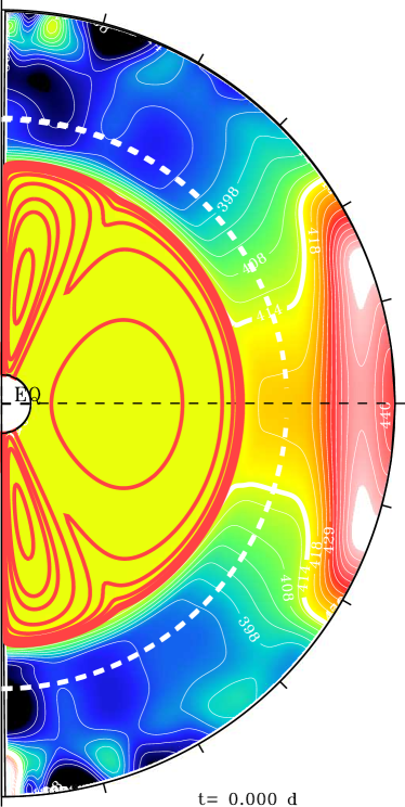
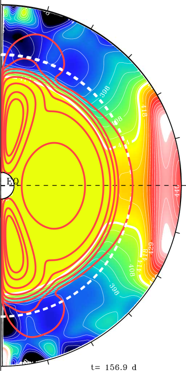
Figure 2: Azimuthal averages of the angular velocity $\Omega$ (color map) and the magnetic field lines (red lines), in the axisymmetric case. The $\Omega$ contours have also been temporally averaged.

Nevertheless, the end state in this case will be the same than in SBZ11. Even if a longer time is needed for the magnetic field lines to interact with the convective motions at the equator, the modified dipole is still axisymmetric. As a result, its interaction with the convective zone will be similar to the behavior described in SBZ11. Angular momentum will still be transported along the field lines, although slight differences may occur due to the little topological change in the bulk of the radiative zone. This will result again in a differentially rotating radiative zone. In the end, the magnetic scenario for the solar tachocline will again certainly fail in this case.

3.2 Non axisymmetric magnetic topology: the oblique dipole

The oblique magnetic fields in stars have been a longstanding subject of research (Mestel and Takhar 1972; Mestel and Weiss 1987). For example, A-type stars are typically thought to be oblique rotators (Brun et al. 2005). Given that a purely axisymmetric field establishes Ferraro’s law, one may wonder whether an oblique dipole acts similarly. In addition, any confined dipolar magnetic field may explain the solid body rotation of the radiation zone. We consequently test the robustness of the results of SBZ11 by considering a tilted dipole.

We use the ASH formalism and decompose the magnetic field into poloidal and toroidal components,

$$\mathbf{B}=\boldsymbol{\nabla}\times\boldsymbol{\nabla}\times\left(C\mathbf{e}_{r}\right)+\boldsymbol{\nabla}\times\left(A\mathbf{e}_{r}\right)\,.$$ (4)

The dipole aligned with the rotation axis is then simply written

$$\left\{\begin{array}[]{lcl}A&=&0\\ C&=&f(r)Y_{0}^{1}\end{array}\right.\,,$$ (5)

where $Y_{l}^{m}$ stands for the classical spherical harmonics. To tilt the dipole with an angle $\beta$ with respect to the rotation axis, we simply write

$$\left\{\begin{array}[]{lcl}A&=&0\\ C&=&f(r)\left(\cos\beta Y_{0}^{1}+\frac{\sin\beta}{\sqrt{2}}Y_{1}^{1}\right)\end{array}\right.\,,$$ (6)

where $f(r)=B_{0}\left(r/R_{\odot}\right)^{2}\left(r-R_{b}\right)^{2}$ and $R_{b}=0.57\,R_{\odot}$ is the bounding radius of the initial magnetic field. We choose $\beta=60^{\circ}$ to tilt significantly the dipole. A 3D rendering of the magnetic field lines is displayed in Fig. 3.

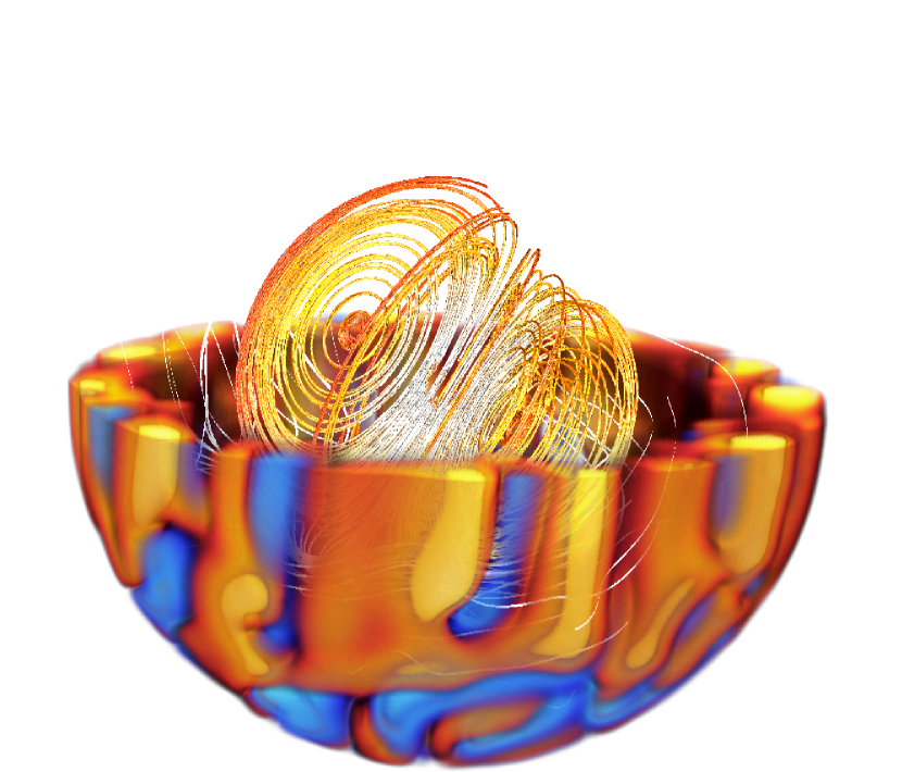
Figure 3: 3D rendering of magnetic field lines. The volume rendering is the azimuthal velocity in the rotating frame in the south hemisphere, orange denotes positive $v_{\varphi}$ and blue negative $v_{\varphi}$.

Although the magnetic topology is clearly different from SBZ11, we observe that if $\beta\neq 90^{\circ}$, then the initial magnetic field is the sum of an axisymmetric dipole (i.e., similar to SBZ11) and a non-axisymmetric component (see eq. (6)). This is also made clear by comparing Figs. 4 and 4 which are taken at the initialization of the magnetic field. The azimuthally averaged field displayed in Fig. 4 only retains the axisymmetric component of the tilted dipole, although the real magnetic configuration is oblique (Fig. 4).

Figs. 4 is taken $\sim 70$ convective turnover times later. We see that the axisymmetric component of the oblique dipole roughly evolves similarly to the pure axisymmetric dipole of SBZ11. We observe indeed that the initially buried magnetic field does not remain confined and connects the convection zone with the radiative interior. The non axisymmetric field likewise does not remain confined in Fig. 4, and its evolution is highly three dimensional. We stress that the field lines plotted in the radiation zone are a fair representation of the field topology, whereas in the tachocline and in the convection zone only the projection into the meridional plane of a 3D magnetic field with non zero azimuthal component is represented.

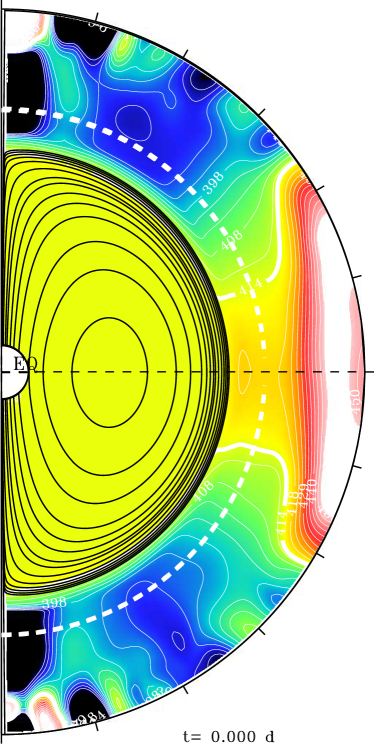
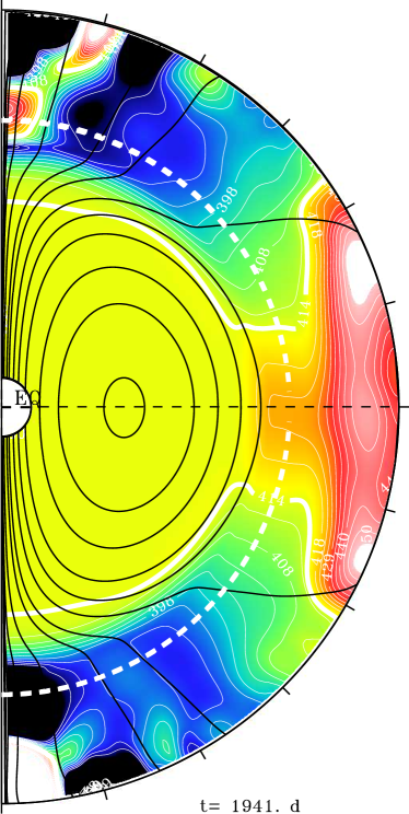
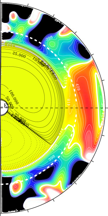
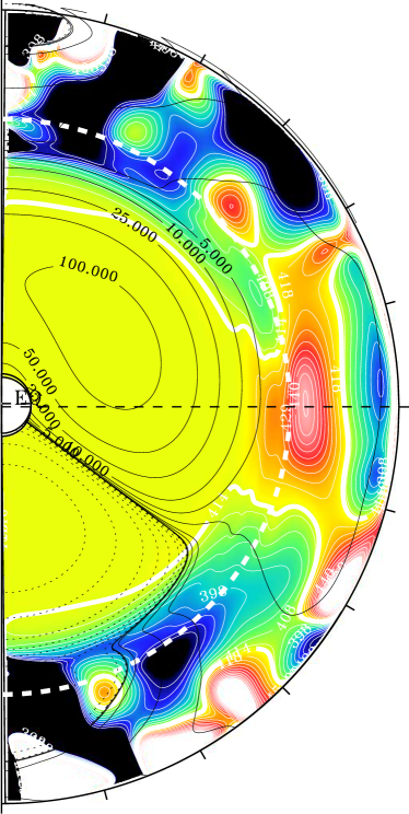
Figure 4: Meridional cuts of the titled dipole case. The quantities in (a,b) are azimuthally averaged, while they are taken at the longitude $\varphi\sim 0$ (i.e., the longitude where the projection of the magnetic field on a polar slice is indeed a planar dipole, at least initially) in panels (c,d). The slight discrepancy between the dipole angle and $60^{\circ}$ (or $-30^{\circ}$) is due to the fact that we are not exactly at $\varphi=0$. The color maps display the angular velocity $\Omega$, and the black lines the magnetic field lines. (a,c) are taken at the initialization of the magnetic field, and (b,d) approximately $70$ convective turnover times later.

The magnetic Reynolds number realized in the convection zone is below the threshold for a dynamo to occur ($Rm\sim 100$ vs $300$ in Brun et al. (2004)). As a result, the total magnetic energy decreases as the simulation evolves.

The polar slices in Fig. 4 seem to exhibit major changes in the $\Omega$ profile at the poles, and we know from SBZ11 that the unconfined axisymmetric magnetic field will apply a torque leading to efficient transport of angular momentum. The evolution of the non-axisymmetric component may also have some effects on the angular momentum balance. Thus we examine the different terms of the angular momentum balance which are defined as follows (Brun et al. 2004):

$$\partial_{t}(\bar{\rho}\mathcal{L})=-\mbox{\boldmath$\nabla$}\cdot(\underbrace{\mathbf{F}^{MC}+\mathbf{F}^{RS}+\mathbf{F}^{VD}}_{\mbox{Hydro}}+\underbrace{\mathbf{F}^{MT}+\mathbf{F}^{MS}}_{\mbox{MHD}})\,,$$ (7)

where the different terms correspond respectively to contributions from Meridional Circulation, Reynolds Stress, Viscous Diffusion, Maxwell Torque and Maxwell Stress. They are defined by

$$\mathbf{F}^{MC} \equiv \bar{\rho}\langle\mathbf{v}_{M}\rangle\mathcal{L}\,,$$ (8)

$$\mathbf{F}^{RS} \equiv r\sin\theta\bar{\rho}\left(\langle v_{r}^{\prime}v_{\varphi}^{\prime}\rangle\mathbf{e}_{r}+\langle v_{\theta}^{\prime}v_{\varphi}^{\prime}\rangle\mathbf{e}_{\theta}\right)\,,$$ (9)

$$\mathbf{F}^{VD} \equiv -\nu\bar{\rho}r^{2}\sin\theta\left\{\partial_{r}\left(\frac{\langle v_{\varphi}\rangle}{r}\right)\mathbf{e}_{r}+\partial_{\theta}\left(\frac{\langle v_{\varphi}\rangle}{\sin\theta}\right)\mathbf{e}_{\theta}\right\}\,,$$ (10)

$$\mathbf{F}^{MT} \equiv -\frac{r\sin\theta}{4\pi}\langle B_{\varphi}\rangle\langle\mathbf{B}_{M}\rangle\,\mathrm{and}$$ (11)

$$\mathbf{F}^{MS} \equiv -\frac{r\sin\theta}{4\pi}\left(\langle B_{r}^{\prime}B_{\varphi}^{\prime}\rangle\mathbf{e}_{r}+\langle B_{\theta}^{\prime}B_{\varphi}^{\prime}\rangle\mathbf{e}_{\theta}\right)\,,$$ (12)

where the subscript $._{M}$ designates the meridional component of $\mathbf{v}$ and $\mathbf{B}$. In the previous equations, we have decomposed the velocity and the magnetic field into an azimuthally averaged part $\langle.\rangle$ and $\varphi$-dependent part (with a prime). The different contributions can further be separated between radial ($\mathcal{F}_{r}$ along $\mathbf{e}_{r}$) and latitudinal ($\mathcal{F}_{\theta}$ along $\mathbf{e}_{\theta}$) contributions. However here we only focus on the radial flux of angular momentum defined by

$$\mathcal{I}_{r}(r) = \int_{\theta_{1}}^{\theta_{2}}\mathcal{F}_{r}(r,\theta)r^{2}\sin\theta\hskip 5.69046pt\mbox{d}{\theta}$$ (13)

where $(\theta_{1},\theta_{2})$ maybe chosen to study a particular region of our simulation.

We plot in Fig. 5 the time-averaged angular momentum balance near the north pole and near the equator about $75$ convective turnover times after the introduction of the magnetic field. The magnetic contributions are highlighted in red and are separated in axisymmetric (Maxwell torque MT) and non axisymmetric (Maxwell stress MS). At the beginning, those contributions are exactly zero. Since the field is initially buried deep in the radiation zone, we first notice that angular momentum is transported at the top of the radiative zone by (axisymmetric) Maxwell torque at the north pole (as already noticed in SBZ11). This again leads to a differentially rotating radiative zone. What is remarkable here is that we also observe magnetic transport of angular momentum at the equator. The axisymmetric and non-axisymmetric (torque and stress) components contribute equally to the inward transport of angular momentum, thus accelerating the upper radiation zone at low latitude, while Maxwell torque slows down the high latitude. We can thus conclude that an oblique field is acting very similarly to a purely aligned dipole.

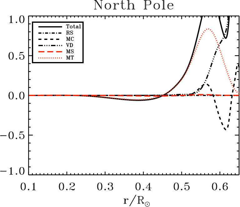
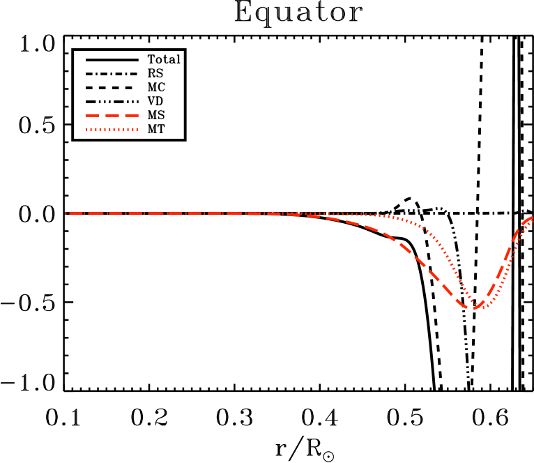
Figure 5: Time-averaged angular momentum balance ($\mathcal{I}_{r}$) at the north pole $(\theta_{1}=60,\theta_{2}=90$, see eq. (13)) and at the equator $(\theta_{1}=-15,\theta_{2}=15)$. $\mathcal{I}_{r}$ is normalized to $10^{12}$.

4 Conclusions and Perspectives

In a previous paper (SBZ11), we tested the Gough and McIntyre (1998) magnetic confinement scenario of the solar tachocline with a 3D non-linear MHD model of $90\%$ of the Sun which couples together the convective and radiative zones. We showed that a fossil axisymmetric magnetic field does not remain confined in the radiation zone, and thus cannot prevent the spread of the tachocline.

We showed that the motions (both meridional circulation and convection) were not strong enough to confine the field and that upward motions at the base of the convection zone were on the contrary helping the field to expand inside the convection zone. Although our numerical experiment is far from representing the real Sun, we are confident that our parameter regime allows us to model the main ingredients of the tachocline confinement scenario. More precisely, we demonstrated in SBZ11 that even if we consider high magnetic diffusivity, our magnetic Reynolds number is higher than $1$ in the overshooting/penetration region and in the convection zone. The magnetic field evolution is thus dominated by advection and not by diffusion. The overshooting depth of the convective plumes is likely to be overestimated because our Peclet number is lower than the solar one, and the penetration of the meridional circulation may be underestimated (see Garaud and Brummell 2008; Wood et al. 2011) in our model. However, penetration and overshooting are clearly observed in our model. If more ’realistic’ values of the parameters could have consequences on the polar dynamics, we stress here that it may not have much influence at the equator, where the confinement of the magnetic field fails.

The magnetic topology considered in SBZ11 was very simple (axisymmetric dipole), and the robustness of the results is not obvious when considering the geometry of the field. We demonstrated in Sect. 3.1 that an axisymmetric dipole preferentially diffuses at the location where its maximum radial gradient is, i.e., at the equator. This has some importance since SBZ11 showed that the lack of confinement specifically at the equator was responsible for the failure of the Gough and McIntyre (1998) scenario. In order to test other topologies, we reported in Sect. 3.2 the study of an oblique dipole buried in the radiation zone. A tilted dipole can be decomposed into an axisymmetric and a non-axisymmetric part, and the axisymmetric component was shown to evolve similarly to the purely axisymmetric dipole of SBZ11. As a result, the magnetic confinement also fails for the tilted dipole.

The non-axisymmetric component of the titled dipole exhibits interesting three dimensional dynamics and transports angular momentum at the equator. In order to get rid of the SBZ11 dynamics and to isolate the effect of the non-axisymmetric dipole, simulations with a purely perpendicular dipole (i.e., with no axisymmetric component, $\beta=90$ in Eq. (6)) will be reported in a future paper.

References

- Brown et al. (1989) Brown, T. M., Christensen-Dalsgaard, J., Dziembowski, W. A., Goode, P., Gough, D. O., and Morrow, C. A.: 1989, ApJ 343, 526
- Brun et al. (2005) Brun, A. S., Browning, M. K., and Toomre, J.: 2005, ApJ 629, 461
- Brun et al. (2004) Brun, A. S., Miesch, M. S., and Toomre, J.: 2004, ApJ 614(2), 1073
- Brun et al. (2011) Brun, A. S., Miesch, M. S., and Toomre, J.: 2011, ApJ, in press
- Brun and Toomre (2002) Brun, A. S. and Toomre, J.: 2002, ApJ 570, 865
- Brun and Zahn (2006) Brun, A. S. and Zahn, J.-P.: 2006, A&A 457, 665
- Charbonneau et al. (1999) Charbonneau, P., Christensen-Dalsgaard, J., Henning, R., Larsen, R. M., Schou, J., Thompson, M. J., and Tomczyk, S.: 1999, ApJ 527(1), 445
- Dorch and Nordlund (2001) Dorch, S. B. F. and Nordlund, Å.: 2001, A&A 365, 562
- Dritschel and McIntyre (2008) Dritschel, D. G. and McIntyre, M. E.: 2008, Journal of the Atmospheric Sciences 65, 855
- Elliott (1997) Elliott, J. R.: 1997, A&A 327, 1222
- Ferraro (1937) Ferraro, V. C. A.: 1937, MNRAS 97, 458
- Garaud (2002) Garaud, P.: 2002, MNRAS 329, 1
- Garaud and Brummell (2008) Garaud, P. and Brummell, N. H.: 2008, ApJ 674(1), 498
- Garaud and Garaud (2008) Garaud, P. and Garaud, J.-D.: 2008, MNRAS 391, 1239
- Gilman and Glatzmaier (1981) Gilman, P. A. and Glatzmaier, G. A.: 1981, ApJ Supp. Series 45, 335