The World-Line Quantum Mechanics Model at Finite Temperature which is Dual to the Static Patch Observer in de Sitter Space

Abstract

A simple conformal quantum mechanics model of a d-component variable is proposed, which exactly reproduces the retarded Green functions and conformal weights of conformally coupled scalar fields in de Sitter spacetime seen by a static patch observer. It is found that the action integral of this model is automatically expressed by a complex integral over the time variable $t$ along a closed contour in a way which is typical to the Schwinger-Keldysh formalism of a thermofield theory. Hence this model is at finite temperature. The case of conformally coupled scalar fields in 3d Schwarzschild de Sitter space is also considered and then a large-N matrix model is obtained.

1 Introduction

Compared to the well-established AdS/CFT correspondence,[1] [2][3] the de Sitter holography is less understood. At least there are two kinds of de Sitter duality which depend on two types of observers. In the global patch of de Sitter spacetime the boundaries are at the future and past infinity ${\cal I}^{+}$, ${\cal I}^{-}$, and the bulk gravity theory is dual to the conformal field theory at ${\cal I}^{+}$. The metaobserver at ${\cal I}^{+}$ can see all the events there through the wave function of the universe[4]. This type of holography has been developed by means of analogy to AdS/CFT duality. [5][6][7] [8][9]

In the static patch the observer is surrounded by a cosmological horizon. The future infinity ${\cal I}^{+}$ is behind the cosmological horizon and one cannot use ${\cal I}^{+}$ for the holography.[10][11] [12][13][14][15] In this case the dual description of the de Sitter spacetime may be expected for the static patch observer residing at $r=0$. Then, because the (d-1)-sphere in the static patch collapses at $r=0$, dS space may be described by a conformal worldline quantum mechanics at the center of dS space.[16]

In [16] the retarded Green function of scalar field and gravitational fluctuations seen by a static patch observer are studied. For conformally coupled scalar fields and gravitons in four dimensional space it was shown that the retarded Green functions take the scaling form and the scaling exponents and wave functions are controlled by a hidden $SL(2,{\mathbb{R}})$ symmetry. In the general case without conformal invariance it was also observed that there are underlying $SL(2,{\mathbb{R}})\times SL(2,{\mathbb{R}})$ symmetry. They also show how the worldline de Sitter propagators can be reproduced from conformal quantum mechanics and speculate that the static patch of de Sitter spacetime may be dually described in terms of large N quantum mechanics. They also presented a simple free model of large N quantum matrix model. The conformal weights derived from this matrix model in the diagonal approximation, however, do not exactly agree with the de Sitter results for scalar fields with non-conformal coupling $x\neq\frac{1}{2}$.

In this paper a simple conformal quantum mechanics model of d-component variables, $x_{i}(\tau)$ ($i=1,..,d$), is proposed, which exactly reproduces the retarded Green functions and conformal weights of scalar fields with conformal coupling and four dimensional gravitons. First, the model of non-matrix type will be obtained, and then a generalization to a large N matrix model will be also presented. The case of scalar fields in 3d Schwarzschild-de-Sitter space with conformal coupling is also considered.

In de Sitter space an observer is in a thermal bath of particles and the de Sitter space is associated with a de Sitter temperature. Thus the conformal quantum mechanics constructed in this paper is expected to be associated with this temperature. It will be shown that this is indeed the case by demonstrating that the action integral for this quantum mechanics is represented as a contour integral along a contour in the complex-time plane as in the thermofield theory.

This paper is organized as follows. In sec.2 the scaling form of retarded Green function in static patch de Sitter space is reviewed. In sec.3 the conformal quantum mechanics is briefly reviewed. In sec.4 a new conformal quantum mechanics theory which reproduces the conformal weights of the retarded Green function in de Sitter space seen by a static patch oberver is presented. Then the primary states with eigenvalues for the conformal generator $R$ is presented. Lagrangian and Hamiltonian of this conformal quantum mechanics reexpressed in terms of de Sitter time $t$ for the static patch are presented in sec.5. Interestingly, it is shown that the action integral is expressed as a contour integral along a closed contour $C$ in the complex-$t$ plane. Hence the dynamical variables also live on a line parallel to the real axis. This is reminiscent of the Schwinger-Keldysh formalism of thermofield theory. The de Sitter temperature is naturally encoded in the conformal quantum mechanics model. In sec.6 3d Schwarzschild-de Sitter space is considered and the conformal quantum mechnics model which reproduce the conformal weight is considered. In sec.7 a large N matrix model which is dual to the static patch observer is presented. Sec.8 is left for discussions.

2 Retarded Green functions and Conformal Weights

In [16] the propagators of scalar fields seen by a static patch observer in de Sitter spacetime were studied. The static patch coordinate system for (d+1)-dimensional de Sitter spacetime is given by

$$ds^{2}=-f(r)dt^{2}+\frac{1}{f(r)}\,dr^{2}+r^{2}\,d\Omega^{2}_{d-1},$$ (1)

where

$$f(r)=1-\left(\frac{r}{\ell}\right)^{2}$$ (2)

with $\ell$ related to the cosmological constant $\Lambda$ by $\Lambda=(d-1)(d-2)/2\ell^{2}$ and $d\Omega_{d-1}^{2}$ the round metric on $S^{d-1}$. There is a cosmogical horizon at $r=\ell$ and the observer is at $r=0$. The symmetry of this metric is $SO(d)\times{\mathbb{R}}_{t}$.

In [16] the wave equation for a free scalar field in the static patch, $\Delta\Phi=m^{2}\,\Phi$, was studied and its retarded Green function was obtained. The mass $m$ of the scalar field is parametrized by

$$\ell^{2}\,m^{2}=\frac{d^{2}}{4}-x^{2}$$ (3)

and $x=1/2$ corresponds to the conformal coupling. In the case of conformally coupled scalar fields the retarded Green function of the operator of an $SO(d)$ angular momentum $l$ was shown to have the form.

$$G^{R}_{l}(t)\propto\theta(t)\left(\frac{\ell^{-1}}{\sinh\frac{1}{2}t/\ell}\right)^{2\Delta},$$ (4)

where the conformal weight was found to be

$$\Delta=l+\frac{1}{2}\,(d-1).$$ (5)

The poles of the retarded Green functions with a complex frequency $\omega$ give the quasi-normal modes. It was shown that the wave functions of the quasi-normal modes are controlled by a hidden $SL(2,{\mathbb{R}})$ symmetry. The conformal weight (5) is found to be related to the Casimir operator ${\cal C}$ of the $SL(2,{\mathbb{R}})$ algebra acting on the wave functions of the quasi-normal modes by the formula ${\cal C}=\Delta(\Delta-1)$. This allows one to associate each mode $l$ of the scalar field to a dual operator with conformal weight $\Delta$. A similar analysis for the gravitational perturbation was also reported. Especially in four dimensional de Sitter spacetime the scaling dimesions of the operators are given by exactly the same expression as (5).

It is also pointed out that this $SL(2,{\mathbb{R}})$ symmetry has an origin in $AdS_{2}\times S^{d-1}$, which is the conformally rescaled metric of de Sitter spacetime.

3 Conformally Invariant Quantum Mechanics

In [16] it was also studied how the structure of the retarded Green function in the case of the conformally coupled scalar fields is reproduced by a dual conformal quantum mechanics theory on the worldline on the static observer in de Sitter spacetime. A free theory example of a conformal quantum mechanics theory of a large N matrix was prorposed. By analogy with the established AdS/CFT dualities it is expected in [16] that the dual worldline theory should be a large N matrix theory. It was shown that in this free theory the scaling dimension, or the lowest eigenvalues of an operator $R$, which will be explained below, (11), takes the value $r_{0}=dN/2+l/2$. Here $N$ is the number of eigenvalues of the matrix variable. It is argued that this value $r_{0}$ corresponds to a lowest weight representation of $SL(2,{\mathbb{R}})\times SL(2,{\mathbb{R}})$. However, the exact coincidence was not observed.

In the following section a conformal quantum mechanics theory of a $d$-component variable $x_{i}$, ($i=1,2,...,,d$) will be presented and it will be shown that this theory reproduces the conformal weight (5). This theory is not a large N-matrix theory. However, an extension to a matrix theory will be discussed in sec 6. Meanwhile, in this section conformally invariant quantum mechanics theory will be briefly reviewed.

Conformally invariant quantum mechanics was studied in [17], and recently in [18] in the context of $AdS_{2}/CFT_{1}$ correspondence. The simplest model is the one with the coordinate $q(\tau)$. $\tau$ is the time variable. The Lagrangian is given by

$$L=\frac{1}{2}\,\dot{q}^{2}-\frac{g}{2q^{2}}.$$ (6)

Here $\dot{q}=dq/d\tau$ and $g$ is a dimensionless constant. This model is invariant under a time translation ($H:\tau\rightarrow\tau+\epsilon$), dilatation ($D:\tau\rightarrow\tau+\epsilon\tau$) and conformal transformation ($K:\tau\rightarrow\tau+\epsilon\tau^{2}$). ($\epsilon$ is an infinitesimal constant parameter.) Under these transformations $q(\tau)$ changes as follows.

$$\delta_{H}q = \epsilon\,\partial_{\tau}q,$$ (7)

$$\delta_{D}q = \epsilon(\tau\partial_{\tau}q-\frac{1}{2}\,q),$$ (8)

$$\delta_{K}q = \epsilon(\tau^{2}\,\partial_{\tau}q-\tau q)$$ (9)

The action integral is invariant, and the corresponding conserved charges $H$, $D$ and $K$ satisfy the $SL(2,{\mathbb{R}})$ algebra.

$$[D,K]=iK,$$

$$[H,K]=2iD,$$

$$[H,D]=iH$$ (10)

The charges can be presented in another basis.

$$R=\frac{1}{2}\,(\ell H+\ell^{-1}K),\qquad L_{\pm}=\pm iD+\frac{1}{2}(\ell^{-1}K-\ell H)$$ (11)

The new charges satisfy

$$[R,L_{\pm}]=\pm L_{\pm},\qquad[L_{-},L_{+}]=2R.$$ (12)

The operator $R$ can be taken to be a positive operator and the above algebra shows that its eigenvalues are integrally spaced. So $R$ can be used to classify the normalizable states. $L_{+}$ and $L_{-}$ are raising and lowering operators. The eigenstates of $R$ are defined by

$$R\,|r\rangle=r\,|r\rangle,$$ (13)

and the primary states satisfy an additional constraint.

$$L_{-}\,|r_{0}\rangle=0$$ (14)

The eigrnvalue of $R$, $r$, takes the values $r=r_{n}=r_{0}+n$, ($n=0,1,2,...$).

The Lie algebra (10) posseses a Casimir operator.

$${\cal C}=\frac{1}{2}\,(HK+KH)-D^{2}$$ (15)

On the tower of eigenstates $|r_{n}\rangle$ it takes a constant value.

$${\cal C}\,|r_{n}\rangle=r_{0}\,(r_{0}-1)\,|r_{n}\rangle$$ (16)

The $SL(2,{\mathbb{R}})$-invariant time evolution of the primary state $|r_{0}\rangle$ with respect to $H$ can be introduced as follows.

$$|r_{0},\tau\rangle=N(\tau)\,e^{-\omega(\tau)\,L_{+}}\,|r_{0}\rangle$$ (17)

Here the functions are

$$N(\tau)=\sqrt{\Gamma(2r_{0})}\,\left(\frac{\omega(\tau)+1}{2}\right)^{2r_{0}},\qquad\omega(\tau)=\frac{\ell+i\tau}{\ell-i\tau}.$$ (18)

One can show that this time-evolved state starts at an imaginary time.

$$|r_{0},\tau\rangle\propto e^{iH\tau}\,e^{\ell H}\,|r_{0}\rangle$$ (19)

By expanding the state (17) in terms of $|r_{n}\rangle$ the correlator is calculated as

$$\langle r_{0},\tau^{\prime}|r_{0},\tau\rangle=\frac{\Gamma(2r_{0})\,\ell^{2r_{0}}}{[2i(\tau^{\prime}-\tau)]^{2r_{0}}}.$$ (20)

This does not agree yet with the scaling correlator obtained from the retarded Green function (4) of the conformally coupled scalar field in de Sitter space. In addition to the ‘scaling time’ $\tau$, it is necessary to introduce ‘de Sitter time’ $t$ defined by [16]

$$\tau=\ell\,\tanh\frac{t}{2\ell}.$$ (21)

The evolution along time $t$ is generated by a new Hamiltonian [16]

$$H_{0}=\frac{1}{2}\,(H-\ell^{-2}K)=H-\ell^{-1}R.$$ (22)

The relation (21) is substituted into (20). Then one obtains

$$\langle r_{0},\tau^{\prime}|r_{0},\tau\rangle=\frac{\Gamma(2r_{0})}{(2i)^{2r_{0}}}\ \left[\frac{\cosh\frac{t^{\prime}}{2\ell}\,\cosh\frac{t}{2\ell}}{\sinh\frac{1}{2\ell}\,(t-t^{\prime})}\right]^{2r_{0}}.$$ (23)

This is still different from (4). For an exact agreement the state $|r_{0},\tau\rangle$ must be rescaled by a certain factor,

$$|r_{0},t\rangle_{dS}=(2d\tau/dt)^{r_{0}}\,|r_{0},\tau\rangle=\left[1-\left(\frac{\tau}{\ell}\right)^{2}\right]^{r_{0}}\,|r_{0},\tau\rangle.$$ (24)

Then one obtains

$${}_{dS}\langle r_{0},t^{\prime}|r_{0},t\rangle_{dS}=\frac{\Gamma(2r_{0})}{(2i)^{2r_{0}}}\ \left[\frac{1}{\sinh\frac{1}{2\ell}\,(t-t^{\prime})}\right]^{2r_{0}}.$$ (25)

This coincides with (4) and (5), if one sets $r_{0}=\Delta$.

4 Quantum Mechanics Model Dual to the Static Patch Observer

In this section we will construct a conformal quantum mechanics model which reproduces the $R$ eigenvalues of the primary state, $r_{0}=\Delta=l+(d-1)/2$.

Let us consider a model, which is described by d-vector $x$ with components, $x_{i}(\tau)$ $(i=1,..,d)$. The Lagrangian is given by

$$L=\frac{1}{2}\,\dot{\mbox{\boldmath$x$}}^{2}-\frac{g_{0}}{2}\,\left[\dot{\mbox{\boldmath$x$}}^{2}-\frac{(\mbox{\boldmath$x$}\cdot\dot{\mbox{\boldmath$x$}})^{2}}{\mbox{\boldmath$x$}^{2}}\right]-\frac{g_{1}}{\mbox{\boldmath$x$}^{2}}.$$ (26)

Here $g_{0}$, $g_{1}$ are dimensionless constants. Note also $\dot{x}_{i}=dx_{i}/d\tau$. The momentum conjugate to $x_{i}$ is given by

$$p_{i}=\dot{x}_{i}-g_{0}\left[\dot{x}_{i}-\frac{\mbox{\boldmath$x$}\cdot\dot{\mbox{\boldmath$x$}}}{\mbox{\boldmath$x$}^{2}}\,x_{i}\right].$$ (27)

This relation can be converted into the following relations.

$$\dot{\mbox{\boldmath$x$}}^{2}=\frac{1}{(1-g_{0})^{2}}\,\left[\mbox{\boldmath$p$}^{2}+\frac{g_{0}(g_{0}-2)}{\mbox{\boldmath$x$}^{2}}\,(\mbox{\boldmath$x$}\cdot\mbox{\boldmath$p$})^{2}\right],$$ (28)

$$\frac{1}{\mbox{\boldmath$x$}^{2}}\,(\mbox{\boldmath$x$}\cdot\dot{\mbox{\boldmath$x$}})^{2}=\frac{1}{\mbox{\boldmath$x$}^{2}}\,(\mbox{\boldmath$x$}\cdot\mbox{\boldmath$p$})^{2}$$ (29)

By using these equations one can compute the Hamiltonian.

$$H=\frac{1}{2(1-g_{0})}\,\mbox{\boldmath$p$}^{2}-\frac{g_{0}}{2(1-g_{0})}\,\frac{(\mbox{\boldmath$x$}\cdot\mbox{\boldmath$p$})^{2}}{\mbox{\boldmath$x$}^{2}}+\frac{g_{1}}{\mbox{\boldmath$x$}^{2}}$$ (30)

This theory has an $SL(2,{\mathbb{R}})$ symmetry. Under $SL(2,{\mathbb{R}})$ transformations $x_{i}(\tau)$ changes as follows.

$$\delta_{H}x_{i} = \epsilon\,\partial_{\tau}x_{i},$$

$$\delta_{D}x_{i} = \epsilon(\tau\partial_{\tau}x_{i}-\frac{1}{2}\,x_{i}),$$ (31)

$$\delta_{K}x_{i} = \epsilon(\tau^{2}\,\partial_{\tau}x_{i}-\tau x_{i})$$

The corresponding conserved Noether charges are obtained by the usual method. The Hamiltonian $H$ is given in (30).

$$D = \tau\,H-\frac{1}{4}\,(\mbox{\boldmath$p$}\cdot\mbox{\boldmath$x$}+\mbox{\boldmath$x$}\cdot\mbox{\boldmath$p$}),$$ (32)

$$K = \tau^{2}\,H-\frac{1}{2}\,\tau\,(\mbox{\boldmath$p$}\cdot\mbox{\boldmath$x$}+\mbox{\boldmath$x$}\cdot\mbox{\boldmath$p$})+\frac{1}{2}\,\mbox{\boldmath$x$}^{2}$$ (33)

Now these charges at $\tau=0$ will be considered. The radial coordinate $\rho=\sqrt{\mbox{\boldmath$x$}^{2}}$ is introduced. Then the above charges are represented as

$$H = -\frac{1}{2}\,\left[\frac{\partial^{2}}{\partial\rho^{2}}+\frac{d-1}{\rho}\frac{\partial}{\partial\rho}\right]+\frac{l(l+d-2)}{2(1-g_{0})\rho^{2}}+\frac{g_{1}}{\rho^{2}},$$ (34)

$$D = i\,\left(\frac{1}{2}\,\rho\frac{\partial}{\partial\rho}+\frac{d}{4}\right),$$ (35)

$$K = \frac{1}{2}\ \rho^{2}$$ (36)

Here $l$ is the magnitude of the $SO(d)$ angular momentum and a sector with a fixed $l$ is considered. The operator ordering in the second term of (30) is here defined as $(\mbox{\boldmath$x$}^{2})^{-1}\,(\mbox{\boldmath$x$}\cdot\mbox{\boldmath$p$})^{2}=-(\partial_{\rho}^{2}+(d-1)\rho^{-1}\partial_{\rho})$. With this definition the resulting charges are hermitian and obey the correct $SL(2,{\mathbb{R}})$ Lie algebra (10).

The Casimir operator (15) takes a constant value in the sector with a fixed $l$. By using (34)-(36) this value is evaluated as

$${\cal C}=\frac{1}{16}\,d(d-4)+\frac{1}{4}\,\frac{l(l+d-2)}{1-g_{0}}+\frac{1}{2}\,g_{1}.$$ (37)

The value of ${\cal C}$ is related as in (16) to the lowest eigenvalue of $R$ by ${\cal C}=r_{0}(r_{0}-1)$. By considering ${\cal C}+\frac{1}{4}$, the following equation is obtained

$$(r_{0}-\frac{1}{2})^{2}=\frac{1}{16}\,(d-2)^{2}+\frac{1}{4}\,\frac{l(l+d-2)}{1-g_{0}}+\frac{1}{2}\,g_{1}.$$ (38)

Then it is easy to see that in order to have a solution

$$r_{0}=l+\frac{d-1}{2}$$ (39)

$g_{0}$ and $g_{1}$ must take the following values.

$$g_{0}=\frac{3}{4},\qquad g_{1}=\frac{3}{8}\,(d-2)^{2}$$ (40)

To summarize the model Lagrangian which gives the appropriate lowest weight of $R$ is the following.

$$L=\frac{1}{8}\,\dot{\mbox{\boldmath$x$}}^{2}+\frac{3}{8}\,\frac{(\mbox{\boldmath$x$}\cdot\dot{\mbox{\boldmath$x$}})^{2}}{\mbox{\boldmath$x$}^{2}}-\frac{3}{8}\,\frac{(d-2)^{2}}{\mbox{\boldmath$x$}^{2}}$$ (41)

The correlater (20) of the R-primary states can be calculated from (41). With the change of time variable to the de Sitter time $t$ (21) and rescaling of the state (24), one obtains the correlator (25).

Now the wave functions for the primary states will be computed. In the $\rho(=\sqrt{\mbox{\boldmath$x$}^{2}})$ representation the charges $R$, $L_{\pm}$ are represented as follows.

$$R = \frac{1}{2}\,(\ell^{-1}K+\ell H)$$ (42)

$$= \frac{1}{4\ell}\,\rho^{2}-\frac{1}{4}\,\left[\partial_{\rho}^{2}+\frac{d-1}{\rho}\,\partial_{\rho}\right]+\frac{l(l+d-2)}{\rho^{2}}+\frac{3}{16\rho^{2}}\,(d-2)^{2},$$

$$L_{\pm} = \pm iD-R+\ell^{-1}K=\mp\frac{1}{2}\left(\rho\,\partial_{\rho}+\frac{d}{2}\right)-r_{n}+\frac{1}{2\ell}\,\rho^{2}$$ (43)

The operator $R$ in the second equation is replaced by its eigenvalue $r_{n}$ on $|r_{n}\rangle$. Separating variables using $SO(d)$ spherical harmonics $Y_{l}(\Omega)$,

$$\Psi(\rho,\Omega)=\psi_{l}(\rho)\,Y_{l}(\Omega),$$ (44)

the normalized primary state $\psi_{l0}(\rho)$ which obeys $L_{-}\psi_{l0}=0$ can be solved and given by

$$\psi_{l0}(\rho)=\sqrt{\frac{\Gamma(d/2)}{\Gamma(2r_{0})\,\pi^{d/2}}}\ \rho^{-\frac{d}{2}}\,\left(\frac{\rho^{2}}{\ell}\right)^{r_{0}}\,e^{-\frac{\rho^{2}}{2\ell}}.$$ (45)

Here $r_{0}$ is given by (39). The descendants $\psi_{ln}(\rho)$ ($n\geq 1$) are obtained by applying the raising operator $L_{+}$ repeatedly on $\psi_{l0}(\rho)$, or by solving the equation $R\,\psi_{ln}=r_{n}\,\psi_{ln}$, and are given by the associated Laguerre polynomial as in [18].

$$\psi_{ln}(\rho)=\sqrt{\frac{n!\ \Gamma(d/2)}{\Gamma(n+2r_{0})\,\pi^{d/2}}}\ \rho^{-\frac{d}{2}}\,\left(\frac{\rho^{2}}{\ell}\right)^{r_{0}}\,e^{-\frac{\rho^{2}}{2\ell}}\,L^{(2r_{0}-1)}_{n}\left(\frac{\rho^{2}}{\ell}\right)$$ (46)

These states are the dual to the quasi-normal modes of the scalar fields in the static patch of de Sitter spacetime. The $R$-eigenvalue of the state (45) can be also obtained by computing $R\,\psi_{l0}(\rho)$ and agrees with $r_{0}=l+\frac{d-1}{2}$.

5 Transformation to the De Sitter Time $t$ and Schiwinger-Keldysh Formalism

Up to now the Lagrangian (41) of the conformal quantum mechanics was expressed in terms of the scaling time $\tau$. Now the Lagrangian expressed by using the de Sitter time $t$ will be studied. This is done by using the relation (21).

One must notice that due to the Jacobian factor $d\tau/dt$ the new Lagrangian $L_{dS}$ is related to the old one by $L_{dS}=L/(2\cosh^{2}\frac{t}{2\ell})$. The variable $x_{i}(\tau)$ is also rescaled as follows.

$$x_{i}(\tau)=\left(2\,\frac{d\tau}{dt}\right)^{\frac{1}{2}}\,\tilde{x}_{i}(t)=\left(\cosh^{2}\frac{t}{2\ell}\right)^{-\frac{1}{2}}\,\tilde{x}_{i}(t)$$ (47)

After a bit of calculation the new Lagrangian is obtained.

$$L_{dS} = \frac{1}{4}\,\left(\frac{d\mbox{\boldmath$\tilde{x}$}}{dt}\right)^{2}+\frac{3}{4}\,\frac{1}{\mbox{\boldmath$\tilde{x}$}^{2}}\,\left(\mbox{\boldmath$\tilde{x}$}\cdot\frac{d\mbox{\boldmath$\tilde{x}$}}{dt}\right)^{2}-\frac{3}{16}\,\frac{(d-2)^{2}}{\mbox{\boldmath$\tilde{x}$}^{2}}+\frac{1}{4\,\ell^{2}}\,\tilde{\mbox{\boldmath$x$}}^{2}$$ (48)

$$-\frac{1}{2\ell}\,\frac{d}{dt}\left(\tanh\frac{t}{2\ell}\ \tilde{\mbox{\boldmath$x$}}^{2}\right)$$

The last term can be dropped, being a total derivative. By the conformal transformation (47) the kinetic term for $x$ does not take a $t$-dependent factor. The action integral obtained from this Lagrangian should be certainly $SL(2,{\mathbb{R}})$ invariant, because this was derived from the invariant Lagrangian (41) by a change of the time variable, but this symmetry is implicitly realized compared to (31).

$$\delta_{H}\,\tilde{x}_{i} = \epsilon\,\left(2\partial_{t}\tilde{x}_{i}\,\cosh^{2}\frac{t}{2\ell}\ -\frac{1}{2\ell}\,\tilde{x}_{i}\,\sinh\frac{t}{\ell}\ \right),$$

$$\delta_{D}\,\tilde{x}_{i} = \epsilon\,\left(\partial_{t}\,\tilde{x}_{i}\,\sinh\frac{t}{\ell}-\frac{1}{2\ell}\,\tilde{x}_{i}\,\cosh\frac{t}{\ell}\right),$$ (49)

$$\delta_{K}\,\tilde{x}_{i} = \epsilon\,\left(2\,\partial_{t}\,\tilde{x}_{i}\,\sinh^{2}\frac{t}{2\ell}\ -\frac{1}{2\ell}\ \tilde{x}_{i}\,\sinh\frac{t}{\ell}\right)$$

Note that the time translation $t\rightarrow t+\epsilon$ corresponds to the combination, $(1/2)(\delta_{H}-\delta_{K})$.

The Hamiltonian is found to have the following form.

$$H_{dS}=\tilde{\mbox{\boldmath$p$}}^{2}-\frac{3}{4}\,\frac{1}{\tilde{\mbox{\boldmath$x$}}^{2}}\,(\tilde{\mbox{\boldmath$x$}}\cdot\tilde{\mbox{\boldmath$p$}})^{2}+\frac{3}{16}\,(d-2)^{2}\,\frac{1}{\tilde{\mbox{\boldmath$x$}}^{2}}-\frac{1}{4\ell^{2}}\,\tilde{\mbox{\boldmath$x$}}^{2}=\frac{1}{2}\,\tilde{H}-\frac{1}{2\ell^{2}}\,\tilde{K}$$ (50)

$\tilde{\mbox{\boldmath$p$}}$ is the momentum conjugate to $\tilde{\mbox{\boldmath$x$}}$. $\tilde{H}$ is (30) with (40) substituted and $x$, $p$ replaced by $\tilde{\mbox{\boldmath$x$}}$ and $\tilde{\mbox{\boldmath$p$}}$. $\tilde{K}$ is obtained from (33) similarly. With the similarly defined $\tilde{D}$, the operators $\tilde{H}$ and $\tilde{K}$ obey the algebra (10). This hamiltonian (50) has a form equal to (22).

If the duality is correct, the conformal quantum mechanics must be at de Sitter temperature. This is encoded in the transformation of the time variables, (21). When the de Sitter time is Wick rotated, $t\rightarrow-it_{E}$, the scaling time is given by

$$\tau=-i\,\ell\,\tan\frac{t_{E}}{2\ell}.$$ (51)

Hence the quantum mechanics theory become periodic in $t_{E}$ with a period $\beta=2\pi\ell$. This is consistent with the expectation that this quantum mechanics is at de Sitter temperature $T_{dS}=\beta^{-1}=1/(2\pi\ell)$.

There is one peculiarity about the time integration contour for the action in the model. The inverse relation of (21),

$$t=\ell\,\log\frac{\ell+\tau}{\ell-\tau},$$ (52)

shows that only the segment of the scaling time, $-\ell\leq\tau\leq\ell$, corresponds to the de Sitter time axis $-\infty<t<\infty$. The remaining regions of $\tau$, $\tau<-\ell$ and $\tau>\ell$, are mapped onto a line $\{t=s-\pi\ell i\,|\,-\infty<s<\infty\}$, which is parallel to the real axis, on the complex-$t$ plane. Hence the line from $\tau=-\infty$ to $\tau=+\infty$ is mapped onto a contour $C$ which goes from $t=-\infty$ to $t=-\infty-2\pi\ell i$ with a detour. It is composed of four parts. See Fig.1.

I.

a path from $t=-\infty$ to $t=+\infty$ along the real axis

II.

a path from $t=+\infty$ to $t=+\infty-\pi\ell i$ along a segment parallell to the imaginary axis

III.

a path from $t=+\infty-\pi\ell i$ to $t=-\infty-\pi\ell i$

IV.

a path from $t=-\infty-\pi\ell i$ to $t=-\infty-2\pi\ell i$ along a segment parallel to the imaginary axis.

This contour $C$ can be made closed by imposing a periodic boundary condition $\tilde{\mbox{\boldmath$x$}}(t+i\,\beta)=\tilde{\mbox{\boldmath$x$}}(t)$ on the variable $\tilde{\mbox{\boldmath$x$}}$.

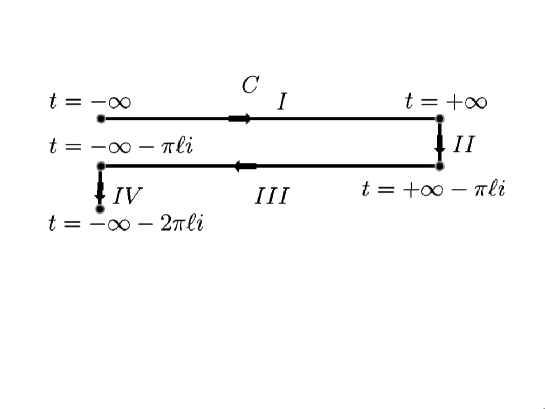
Figure 1: The contour $C$ for the action integral

This contour is reminiscent of the Schwinger-Keldysh formalism of thermofield theory.[19][20] The action integral $S$ obtained by means of the change of variable (21) from $\int_{-\infty}^{\infty}d\tau L(\tau)$ is given by

$$S=\int_{C}dtL_{dS}(t)=\int_{-\infty}^{\infty}dt\,L_{dS}(t)-\int_{-\infty}^{\infty}dt\,L_{dS}(t-\pi\ell i).$$ (53)

The contributions from the segments II, IV are actually absent, being placed at infinities. Hence this conformal quantum mechanics theory turns out to contain twice the real degrees of freedom. The first term on the right side of the above equation corresponds to the real system and the second to its fictitious copy. Actually, the first term will describe the southern causal diamond in the global patch [21], where the observer lives, and the second term the northern causal diamond beyond the cosmological horizon.

In a field theory at finite temperature the original system is doubled.[19][10][20] The doubled system will be described by an entangled state called a thermofield double.

$$|\psi\rangle=\frac{1}{\sqrt{Z}}\,\sum_{i}\,e^{-\frac{1}{2}\beta E_{i}}\,|E_{i}\rangle\otimes|E_{i}\rangle.$$ (54)

Here $Z(\beta)$ is the partition function. The hamiltonian of the thermofield double will be given by $H_{thermo\ double}=H_{dS}\otimes I-I\otimes H_{dS}$ and $E_{i}$ is the eigenvalue of $H_{dS}$. The state $|\psi\rangle$ is an eigenstate of $H_{thermo\ double}$ with an eigenvalue zero. The density matrix $\hat{\rho}$ of the original system is given by computing the trace of $|\psi\rangle\langle\psi|$ over the second Hilbert space of the tensor product. The Green functions of the theory (53) ordered along the contour $C$, the Schwinger-Keldysh correlators, are known to be related to the retarded Green function $\tilde{G}^{R}(\omega)$.[19][20]

There is, however, a problem. The eigenvalues of $H_{dS}$ are not descrete. Furthermore, the potential in (50) is unbounded from below. Then the state $|\psi\rangle$ becomes a pure state with $E_{i}=-\infty$. Because the $SL(2,{\mathbb{R}})$ Casimir is fixed in this theory, this problem might be solved by constructing the thermofield double $|\psi\rangle$ in terms of the eigenstates of the generator $\tilde{R}$. Then it might become possible to compute correlation functions using the thermofield theory. All these issues must be investigated further.

6 Conformal Scalar Field in 3D Schwarzschild-de-Sitter Space

In this section the retarded Green function for a conformally coupled scalar field in 3 dimensional Schwarzschild-de-Sitter space (SdS₃) is considered by using the method of [16] and the corresponding conformally invariant quantum mechanics model is derived.

Schwarzschild-de-Sitter spacetime in d+1 dimensions (SdS_d+1) has the metric

$$ds^{2}=-\tilde{f}(r)\,dt^{2}+\frac{1}{\tilde{f}(r)}\,dr^{2}+r^{2}\,d\Omega_{d-1}^{2},$$ (55)

where

$$\tilde{f}(r)=1-2M\,r^{2-d}-\left(\frac{r}{\ell}\right)^{2}$$ (56)

and $M$ is a constant. When $d=2$ (and $d=1$), the rescaled metric $d\tilde{s}^{2}=ds^{2}/r^{2}$ coincides with that of $AdS_{2}\times S_{d-1}$ and a hidden $SL(2,{\mathbb{R}})$ symmetry can be expected.[16] For $d=2$ the scalar field with angular momentum $l$ in this gravitational background obeys the equation of motion

$$\tilde{f}(r)\,\frac{d^{2}}{dr^{2}}\,\phi(r)+\left(\frac{1-2M}{r}-\frac{3}{\ell^{2}}\,r\right)\,\frac{d}{dr}\phi(r)$$

$$\qquad+\left(-\frac{d^{2}}{4\ell^{2}}+\frac{x^{2}}{\ell^{2}}-\frac{l^{2}}{r^{2}}+\frac{\omega^{2}}{\tilde{f}(r)}\right)\,\phi(r)=0.$$ (57)

Here $\omega$ is the frequency and $x$ is a parameter defined in (3). For the angular momentum $l$ is used instead of $m$ to avoid confusion with the mass.

The angular momentum takes the value $l=0,\pm 1,\pm 2,...$ For $l\neq 0$, there are two solutions, the normalizable and non-normalizable ones, which satisfy the ingoing boundary condition at the cosmological horizon. These are expressed in terms of the hypergeometric functions as follows.

$$\phi_{n.}(r) = (1-z)^{-i\frac{\ell^{2}\omega}{2a}}\,z^{\frac{|l|\ell}{2a}}\,F\left(\alpha_{+},\alpha_{-};\gamma;z\right),$$

$$\phi_{n.n.}(r) = (1-z)^{-i\frac{\ell^{2}\omega}{2a}}\,z^{-\frac{|l|\ell}{2a}}\,F\left(\alpha_{+}-\gamma+1,\alpha_{-}-\gamma+1;2-\gamma;z\right)$$ (58)

Here $z=(r/a)^{2}$ and

$$a=\ell\,\sqrt{1-2M},\qquad\alpha_{\pm}=\frac{1\pm x}{2}+\frac{|l|\ell}{2a}-i\frac{\ell^{2}\omega}{2a},\qquad\gamma=1+\frac{|l|\ell}{a}$$ (59)

In SdS₃ the Hawking temperature is given by $T_{SdS}=a/(2\pi\ell^{2})$.[22] Then the retarded Green function can be calculated as in [16]. For the case of the conformal coupling $x=1/2$ it turns out to be given by

$$G^{R}_{l}(t)\propto\theta(t)\,\left(\frac{1}{\sinh\frac{at}{2\,\ell^{2}}}\right)^{1+\frac{2|l|\ell}{a}}.$$ (60)

To derive this result for the mode $l\,$ ($\neq 0$), one requires that $\phi_{l}=B\,\phi_{n.}+A\,\phi_{n.n.}$ be ingoing at the horizon $z=1$. This determines the ratio $B/A$ and one obtains

$$\tilde{G}^{R}_{l}(\omega)\propto\frac{B}{A}=-\frac{\Gamma(1-\frac{|l|}{a}\ell)}{\Gamma(1+\frac{|l|}{a}\ell)}\,\frac{\Gamma(\frac{1}{2}+\frac{|l|}{a}\ell-i\frac{\ell^{2}}{a}\omega)}{\Gamma(\frac{1}{2}-\frac{|l|}{a}\ell-i\frac{\ell^{2}}{a}\omega)}.$$ (61)

With a non-vanishing $M$ the residues at the poles are regularized.

For the mode $l=0$, the solutions (58) in terms of hypergeometric functions are degenerate and another solution which includes $\log r$ must be taken into account. This case needs some care. For this purpose one rewrites $\phi_{l}$ as

$$\phi_{l} = D\,(1-z)^{-i\frac{\ell^{2}\omega}{2a}}\,z^{\frac{|l|\ell}{2a}}\,F\left(\alpha_{+},\alpha_{-};\gamma;z\right)$$ (62)

$$+C\,\frac{1}{1-\gamma}\,(1-z)^{-i\frac{\ell^{2}\omega}{2a}}\,\left[z^{-\frac{|l|\ell}{2a}}\,F\left(\alpha_{+}-\gamma+1,\alpha_{-}-\gamma+1;2-\gamma;z\right)\right.$$

$$\qquad\qquad\left.-z^{\frac{|l|\ell}{2a}}\,F\left(\alpha_{+},\alpha_{-};\gamma;z\right)\right]$$

Here $C=(1-\gamma)\,A$ and $D=A+B$. One then analytically continues the variable $l$ from an integer variable to a continuous one, and takes the limit $l\rightarrow 0$. Then $\gamma\rightarrow 1$ and one obtains

$$\tilde{G}^{R}_{0}(\omega)\propto\lim_{l\rightarrow 0}\,\frac{D}{C}=2\,\psi\left(\frac{1}{2}-i\frac{\ell^{2}}{a}\omega\right)-\psi(1)-2\,\log 2,$$ (63)

where $\psi(z)$ is a di-gamma function. By discarding the analytic terms, which gives contact terms, and performing Fourier transform, one gets (60) for $l=0$. Note that not only the first term but also the second in (62) is actually normalizable for $l\rightarrow 0$, but the second term represents the source and the first term the response.

From the above result one can read off the conformal weight.

$$\tilde{\Delta}=|l|\,\frac{\ell}{a}+\frac{1}{2}=\frac{|l|}{\sqrt{1-2M}}+\frac{1}{2}$$ (64)

Compared to (5) with $d=2$ substituted, the conformal weight is smoothly deformed by $M$. The conformal quantum mechanics model which reproduces this Green function can be derived by the same procedure as in sec 4. In the present case $r_{0}=\tilde{\Delta}$ and

$$(\tilde{\Delta}-\frac{1}{2})^{2}=\frac{1}{4}\,\frac{l^{2}}{1-g_{0}}+\frac{1}{2}\,g_{1}$$ (65)

This is satisfied, if

$$g_{0}=\frac{3}{4}+\frac{1}{2}\,M,\qquad g_{1}=0.$$ (66)

The corresponding conformal quantum mechanics theory is defined by the Lagrangian

$$L_{SdS_{3}}=\frac{1}{8}\,\dot{\mbox{\boldmath$x$}}^{2}-\left(\frac{3}{8}-\frac{M}{4}\right)\,\frac{(\mbox{\boldmath$x$}\cdot\dot{\mbox{\boldmath$x$}})^{2}}{\mbox{\boldmath$x$}^{2}}.$$ (67)

In the above example a deformation of the background metric of spacetime leads to a deformation of the parameter $g_{0}$ of the conformal quantum mechanics. It can be said that this Lagrangian depends on the Hawking temperature $T_{SdS}$ via the parameter $M$. For higher dimensions ($d>2$) there will be no $SL(2,{\mathbb{R}})$ symmetry. It would be interesting if a non-conformal quantum mechanics model which corresponds to a scalar field in $SdS_{d+1}$ could be found.

7 Large-N Matrix Model

In this section the results of sec.4 are extended to the large N matrix model. It is assumed that the static patch observer is described by N by N hermitian matrices $X^{i}$ ($i=1,..,d$). It may be a gauged D=1 matrix model. In this case the gauge field matrix $A_{\tau}$ can be gauged fixed, $A_{\tau}=0$, and its only role will be to impose a vanishing charge condition $Q=0$ on the state vectors. In the diagonal matrix approximation which will be adopted here, this condition is nothing but the permutation symmetry of the eigenvalues of the matrices. Hence a gauge field will not be considered here.

The following form of the Lagrangian is assumed.

$$L_{M}=\frac{1}{2}\,\mbox{Tr}\sum_{i=1}^{d}\,(\dot{X}^{i})^{2}-\frac{g_{2}}{\mbox{Tr}\,\sum_{i=1}^{d}\,(X^{i})^{2}}$$ (68)

Here $g_{2}$ is a constant. In what follows the diagonal approximation will be adopted, i.e., the matrix $X^{i}$ is assumed to be diagonal. In the classical geometric limit, the off-diagonal matrix elements are assumed to be heavy compared to the diagonal elements. The diagonal elements are denoted as $x_{a}^{i}(\tau)$, ($a=1,2,...,N$). Then the Lagrangian reduces to

$$L_{M}=\frac{1}{2}\,\sum_{a}\,\dot{\mbox{\boldmath$x$}}_{a}^{2}-\frac{g_{2}}{\sum_{a}\mbox{\boldmath$x$}_{a}^{2}}.$$ (69)

The momentum conjugate to $x_{a}^{i}$ is given by $p_{a}^{i}=\dot{x}_{a}^{i}$. The conserved charges at $\tau=0$ are

$$H = \frac{1}{2}\,\sum_{a}\mbox{\boldmath$p$}_{a}^{2}+\frac{g_{2}}{\sum_{a}\mbox{\boldmath$x$}_{a}^{2}},$$ (70)

$$D = -\frac{1}{2}\,\sum_{a}\,\mbox{\boldmath$x$}_{a}\cdot\mbox{\boldmath$p$}_{a},$$ (71)

$$K = \frac{1}{2}\,\sum_{a}\,\mbox{\boldmath$x$}_{a}^{2}$$ (72)

Now it is assumed that the primary state has the wave function,

$$\psi(\mbox{\boldmath$x$}_{a})=\left(\sum_{a}\,c_{i_{1},i_{2},...,i_{l}}\,x_{a}^{i_{1}}\cdots x_{a}^{i_{l}}\right)\ \left(\sum_{b}\mbox{\boldmath$x$}_{b}^{2}\right)^{\alpha}\ \exp\left\{\frac{-1}{2}\ \sum_{c}\mbox{\boldmath$x$}_{c}^{2}\right\}$$ (73)

where $c_{i_{1},..,i_{l}}$ is a constant symmetric traceless tensor, and $\alpha$ is a constant. The lowest-weight condition $L_{-}\,\psi=0$ yields the equation.

$$\alpha=r_{0}-\frac{l}{2}-\frac{1}{4}\,Nd,$$ (74)

where $r_{0}$ is the eigenvalue of $R$. Now the eigenvalue equation $R\psi=r_{0}\psi$ gives

$$R\psi=\frac{1}{4}\,(2l+4\alpha+Nd)\psi+\frac{1}{2\sum_{a}\mbox{\boldmath$x$}_{a}^{2}}\,(g_{2}-2l\alpha-Nd\alpha-2\alpha(\alpha-1))\psi.$$ (75)

From this one obtains two constraints.

$$r_{0} = \frac{1}{4}\,(2l+Nd+4\alpha),$$ (76)

$$g_{2} = (2r_{0}+l+\frac{Nd}{2}-2)(r_{0}-\frac{l}{2}-\frac{1}{4}Nd)$$ (77)

The first equation is consistent with (74). To obtain the eigenvalue $r_{0}=l+\frac{d-1}{2}$ (5), one must set

$$\alpha = \frac{l}{2}+\frac{d-1}{2}-\frac{N}{4}\,d,$$ (78)

$$g_{2} = \frac{3}{2}\,l(l+d-2)-\frac{d}{2}\,(N-1)\,l-\frac{1}{8}\,[Nd+2(d-3)][Nd-2(d-1)]$$ (79)

Note that this value of $\alpha$ ensures the normalizability of $\psi$. One must note that the constant $g_{2}$ should not depend on the angular momentum $l$. So the combination $l(l+d-2)$ is to be relpaced by the squared angular momentum operator,

$$\mbox{\boldmath$L$}^{2}=\sum_{a,b}\,[(\mbox{\boldmath$x$}_{a}\cdot\mbox{\boldmath$x$}_{b})\,(\mbox{\boldmath$p$}_{a}\cdot\mbox{\boldmath$p$}_{b})-(\mbox{\boldmath$x$}_{a}\cdot\mbox{\boldmath$p$}_{a})(\mbox{\boldmath$x$}_{b}\cdot\mbox{\boldmath$p$}_{a})].$$ (80)

The operator ordering must be correctly specified. There is also a linear term of $l$. This must be also replaced by

$$l\rightarrow-\frac{d-2}{2}+\sqrt{\frac{1}{4}(d-2)^{2}+\mbox{\boldmath$L$}^{2}}.$$ (81)

Finally, the hamiltonian $H$ (70) is given by the following complicated expression.

$$H_{M} = \frac{1}{2}\,\sum_{a}\,\mbox{\boldmath$p$}_{a}^{2}+\frac{3}{2\sum_{c}\,\mbox{\boldmath$x$}_{c}^{2}}\,\mbox{\boldmath$L$}^{2}-\frac{d(N-1)}{2\sum_{b}\mbox{\boldmath$x$}_{b}^{2}}\,\sqrt{\frac{(d-2)^{2}}{4}+\mbox{\boldmath$L$}^{2}}$$ (82)

$$+\frac{1}{\sum_{b}\,\mbox{\boldmath$x$}_{b}^{2}}\left[\frac{d(d-2)}{4}(N-1)-\frac{1}{8}\,(Nd+2d-6)(Nd-2d+2)\right].$$

The corresponding Lagrangian $L^{\prime}_{M}$ then differs from (69). This can be obtained by eliminating $p_{a}^{i}$ from $L^{\prime}_{M}=\sum_{a}\dot{\mbox{\boldmath$x$}}_{a}\cdot\mbox{\boldmath$p$}_{a}-H_{M}$. This Lagrangian is implicitly given by

$$L^{\prime}_{M} = \frac{1}{2}\,\sum_{a}\mbox{\boldmath$p$}_{a}^{2}+\frac{1}{\sum_{c}\,\mbox{\boldmath$x$}_{c}^{2}}\,\left[\frac{3}{2}\,\mbox{\boldmath$L$}^{2}+\frac{N-1}{8}\frac{d(d-2)^{2}}{\sqrt{\frac{1}{4}\,(d-2)^{2}+\mbox{\boldmath$L$}^{2}}}\right.$$ (83)

$$\left.-\frac{1}{4}\,d(d-2)(N-1)+\frac{1}{8}\,\{Nd+2d-6)(Nd-2d+2)\}\right],$$

where $p_{a}^{i}$ is determined by solving the following equation for $p_{a}^{i}$

$$\dot{x}_{a}^{i}=p_{a}^{i}+\frac{1}{\sum_{c}\,\mbox{\boldmath$x$}_{c}^{2}}\,\left[3-\frac{d(N-1)}{2}\,\frac{1}{\sqrt{\frac{1}{4}\,(d-2)^{2}+\mbox{\boldmath$L$}^{2}}}\right]\,\sum_{b}\,[(\mbox{\boldmath$x$}_{a}\cdot\mbox{\boldmath$x$}_{b})p_{b}^{i}-(\mbox{\boldmath$x$}_{a}\cdot\mbox{\boldmath$p$}_{b})x_{b}^{i}].$$ (84)

It is straightforward to obtain the matrix form of the Hamiltonian from (82).

8 Discussion

In this paper a simple conformal quantum mechanics model of d-component fields, $x_{i}(\tau)$, ($i=1,..,d$) (41) is proposed, which exactly reproduces the retarded Green functions and conformal weights of scalar fields with conformal coupling and four dimensional gravitons seen by a static patch observer. The model obtained in sec.4 is not of the type of large N matrix model.

In sec.5 the Lagrangian of the quantum mechanics model obtained in the previous section is rewritten in terms of the de Sitter time $t$. It is found that the action integral is given by a contour integral along a closed contour in the complex-$t$ plane. This is nothing but the Schwinger-Keldysh formalism of thermofield theory. Hence the finite temperature is naturally encoded in the conformal quantum mechanics model.

The conformal quantum mechanics model we found is extended to a large N matrix model in sec.7. This model, however, has several problems. The hamiltonian is obtained, but the Lagrangian is complicated and its form is worked out only implicitly. The form of the matrix model Hamiltonian is unusual one with the traces of matrices in the denominators. Although the primary states of the form (73) are uniquely determined and will correspond to the conformally coupled scalar fields in the static patch, there may be more primary states. It is important to identify the whole primary states. In this respect an analysis of the full matrix model is important. On the other hand, the construction of the large N matrix model in sec.7 can be applied to the $x\neq 1/2$ case with $SL(2,{\mathbb{R}})\times SL(2,{\mathbb{R}})$ symmetry.

In sec.6 a conformal quantum mechanics model for a scalar field with a conformal coupling in SdS₃ is constructed and it is found that the Lagrangian depends on the Hawking temperature $T_{SdS}$ via the parameter $M$. A similar analysis can be applied to the $x\neq 1/2$ case with $SL(2,{\mathbb{R}})\times SL(2,{\mathbb{R}})$ symmetry[16] and will lead to an interacting Lagrangian which depends on $T_{SdS}$ or $M$.

References

• [1] J.M. Mardacena, The Large N Limit of Superconformal Field Theories and Supergravity, [arXiv:hep-th/9711200]
• [2] S.S. Gubser, I.R. Klebanov and A.M. Polyakov, Gauge theory Collerators from Non-critical String Theory, [arXiv:hep-th/9802109].
• [3] E. Witten, Anti-de-Sitter Space and Holography, arXiv:hep-th/9802150].
• [4] J. B. Hartle and S. W. Hawking, Wave Function of the Universe, Phys. Rev. D28, 2960-2975 (1983).
• [5] E. Witten, Quantum Gravity in de Sitter Space, [arXiv: hep-th/0106109].
• [6] A. Strominger, The dS/CFT Correspondence, JHEP 0110, 034 (2001), [arXiv:hep-th/0106113].
• [7] J.M. Maldacena, Non-Gaussian Features of Primodial Flictuations in Single Field Inflationary Models, JHEP 0305, 013 (2003), [astro-ph/0210603].
• [8] D. Antonos, G.S. Ng and A. Strominger, Asymptotic Symmetries and Charges in De Sitter Space, [arXiv:1009.4730].
• [9] D. Anninos, T. Hartman and A. Strominger, Higher Spin Realization of the de Sitter Space, [arXiv:1108.5735 [hep-th]].
• [10] N. Goheer, T. Hartman and A. Strominger, The Trouble with de Ditter Space, JHEP 0307, 056 (2003) [hep-th/0212209].
• [11] T. Banks, Some thoughts on the quantum thoery of de sitter space, [astro-ph/0305037].
• [12] M.K.Parikh and E.P. Verlinde, De Sitter Holography with a Finite Number of States, JHEP 0501, 054 (2005), [hep-th/0410227].
• [13] T. Banks, B. Fiol and A. Morisse, Towards a Quantum Theory of de Sitter Space, JHEP 0612, 004 (2006), [hep-th/0609062].
• [14] L. Susskind, Addendum to Fast Scramblers, [arXiv:1101.6048 [hep-th]].
• [15] A. Castro, N. Lashkari and A. Maloney, A de Sitter Farey Tail, Phys. Rev. D83, 124027 (2011), [arXiv:1103.4620 [hep-th]].
• [16] D. Anninos, S.A. Hartnoll and D. M. Hofman, Static Patch Solipsism: Conformal Symmetry of the de Sitter Worldline, [arXiv: 1109.4942 [hep-th]].
• [17] V. de Alfaro, S. Fubini and G. Furlan, Conformal Invariance in Quantum Mechanics, Il Nuovo Cim. 34A (1976) 569.
• [18] C. Chamon, R. Jackiw, S-Y Pi, and L. Santos, Conformal Quantum Mechanics as the CFT1 dual to AdS2, [arXiv:1106.0726].
• [19] P. Martin and J. Schwinger, Phys. Rev. 115 (1959)1342; J. Schwinger, Journal of Mathematical Physics 2 (1961) 407; K.T. Mahantappa, Phys. Rev. 126 (1962) 329; P. M. Bakshi and K. T. Mahantappa, Journal of Mathematical Physics 4 (1963)1 and 12; L. V. Keldysh, Soviet Physics JETP 20 (1965) 1018; Y. Takahashi and H. Umezawa, Collective Phenomena 2 (1975) 55.
• [20] C.P. Herzog and D. T. Son, Schwinger-Keldysh Propagators from AdS/CFT Correspondence, [arXiv: 0212072 [hep-th]].
• [21] M. Spraddlin, A. Strominger and A. Volovich, Les Houches Lectures on de Sitter Space, [arXiv: 0110007 [hep-th]].
• [22] G. W. Gibbons and S. W. Hawking, Cosmological Event Horizons, Thermodynamics, And Particle Creations, Phys. Rev. D15 (1977) 2738.