Steganography: a class of secure and robust algorithms

Abstract

This research work presents a new class of non-blind information hiding algorithms that are stego-secure and robust. They are based on some finite domains iterations having the Devaney’s topological chaos property. Thanks to a complete formalization of the approach we prove security against watermark-only attacks of a large class of steganographic algorithms. Finally a complete study of robustness is given in frequency DWT and DCT domains.

1 Introduction

This work focus on non-blind binary information hiding chaotic schemes: the original host is required to extract the binary hidden information. This context is indeed not as restrictive as it could primarily appear. Firstly, it allows to prove the authenticity of a document sent through the Internet (the original document is stored whereas the stego content is sent). Secondly, Alice and Bob can establish an hidden channel into a streaming video (Alice and Bob both have the same movie, and Alice hide information into the frame number $k$ iff the binary digit number $k$ of its hidden message is 1). Thirdly, based on a similar idea, a same given image can be marked several times by using various secret parameters owned both by Alice and Bob. Thus more than one bit can be embedded into a given image by using this work. Lastly, non-blind watermarking is useful in network’s anonymity and intrusion detection [1], and to protect digital data sending through the Internet [2]. Furthermore, enlarging the given payload of a data hiding scheme leads clearly to a degradation of its security: the smallest the number of embedded bits is, the better the security is.

Chaos-based approaches are frequently proposed to improve the quality of schemes in information hiding [3, 4, 5, 6]. In these works, the understanding of chaotic systems is almost intuitive: a kind of noise-like spread system with sensitive dependence on initial condition. Practically, some well-known chaotic maps are used either in the data encryption stage [4, 5], in the embedding into the carrier medium, or in both [3, 7]. Methods referenced above are almost based on two fundamental chaotic maps, namely the Chebychev and logistic maps, which range in $\mathbb{R}$. To avoid justifying that functions which are chaotic in $\mathbb{R}$ still remain chaotic in the computing representation (i.e., floating numbers) we argue that functions should be iterated on finite domains. Boolean discrete-time dynamical systems (BS) are thus iterated.

Furthermore, previously referenced works often focus on discretion and/or robustness properties, but they do not consider security. As far as we know, stego-security [8] and chaos-security have only been proven on the spread spectrum watermarking [9], and on the dhCI algorithm [10], which is notably based on iterating the negation function. We argue that other functions can provide algorithms as secure as the dhCI one. This work generalizes thus this latter algorithm and formalizes all its stages. Due to this formalization, we address the proofs of the two security properties for a large class of steganography approaches.

This research work is organized as follows. It firstly introduces the new class of algorithms (Sec. 2), which is the first contribution. Next, the Section 3 presents a State-of-the-art in information hiding security and shows how secure is our approach. The proof is the second contribution. The chaos-security property is studied in Sec. 4 and instances of algorithms guaranteeing that desired property are presented. This is the fourth contribution. Applications in frequency domains (namely DWT and DCT embedding) are formalized and corresponding experiments are given in Sec. 5. This shows the applicability of the whole approach. Finally, conclusive remarks and perspectives are given in Sec. 6.

2 Information hiding algorithm: formalization

As far as we know, no result rules that the chaotic behavior of a function that has been established on $\mathbb{R}$ remains on the floating numbers. As stated before, this work presents the alternative to iterate a Boolean map: results that are theoretically obtained in that domain are preserved during implementations. In this section, we first give some recalls on Boolean discrete dynamical Systems (BS). With this material, next sections formalize the information hiding algorithms based on these Boolean iterations.

2.1 Boolean discrete dynamical systems

Let us denote by $\llbracket a;b\rrbracket$ the interval of integers: $\{a,a+1,\ldots,b\}$, where $a\leqslant b$.

Let $n$ be a positive integer. A Boolean discrete-time network is a discrete dynamical system defined from a Boolean map $f:\mathds{B}^{n}\to\mathds{B}^{n}$ s.t.

$$x=(x_{1},\dots,x_{n})\mapsto f(x)=(f_{1}(x),\dots,f_{n}(x)),$$

and an iteration scheme: parallel, serial, asynchronous…With the parallel iteration scheme, the dynamics of the system are described by $x^{t+1}=f(x^{t})$ where $x^{0}\in\mathds{B}^{n}$. Let thus $F_{f}:\llbracket 1;n\rrbracket\times\mathds{B}^{n}$ to $\mathds{B}^{n}$ be defined by

$$F_{f}(i,x)=(x_{1},\dots,x_{i-1},f_{i}(x),x_{i+1},\dots,x_{n}),$$

with the asynchronous scheme, the dynamics of the system are described by $x^{t+1}=F_{f}(s^{t},x^{t})$ where $x^{0}\in\mathds{B}^{n}$ and $s$ is a strategy, i.e., a sequence in $\llbracket 1;n\rrbracket^{\mathbb{N}}$. Notice that this scheme only modifies one element at each iteration.

Let $G_{f}$ be the map from $\mathcal{X}=\llbracket 1;n\rrbracket^{\mathbb{N}}\times\mathds{B}^{n}$ to itself s.t.

$$G_{f}(s,x)=(\sigma(s),F_{f}(s^{0},x)),$$

where $\sigma(s)^{t}=s^{t+1}$ for all $t$ in $\mathbb{N}$. Notice that parallel iteration of $G_{f}$ from an initial point $X^{0}=(s,x^{0})$ describes the “same dynamics” as the asynchronous iteration of $f$ induced by the initial point $x^{0}$ and the strategy $s$.

Finally, let $f$ be a map from $\mathds{B}^{n}$ to itself. The asynchronous iteration graph associated with $f$ is the directed graph $\Gamma(f)$ defined by: the set of vertices is $\mathds{B}^{n}$; for all $x\in\mathds{B}^{n}$ and $i\in\llbracket 1;n\rrbracket$, $\Gamma(f)$ contains an arc from $x$ to $F_{f}(i,x)$.

We have already established [11] that we can define a distance $d$ on $\mathcal{X}$ such that $G_{f}$ is a continuous and chaotic function according to Devaney [12]. The next section focus on the coding step of the steganographic algorithm based on $G_{f}$ iterations.

2.2 Coding

In what follows, $y$ always stands for a digital content we wish to hide into a digital host $x$.

The data hiding scheme presented here does not constrain media to have a constant size. It is indeed sufficient to provide a function and a strategy that may be parametrized with the size of the elements to modify. The mode and the strategy-adapter defined below achieve this goal.

Definition 1 (Mode)

A map $f$, which associates to any $n\in\mathds{N}$ an application $f_{n}:\mathds{B}^{n}\rightarrow\mathds{B}^{n}$, is called a mode. _□

For instance, the negation mode is defined by the map that assigns to every integer $n\in\mathds{N}^{*}$ the function

$${\neg}_{n}:\mathds{B}^{n}\to\mathds{B}^{n},(x_{1},\ldots,x_{n})\mapsto(\overline{x_{1}},\ldots,\overline{x_{n}}).$$

Definition 2 (Strategy-Adapter)

A strategy-adapter is a function $\mathcal{S}$ from $\mathbb{N}$ to the set of integer sequences, which associates to $n$ a sequence $S\in\llbracket 1,n\rrbracket^{\mathds{N}}$. _□

Intuitively, a strategy-adapter aims at generating a strategy $(S^{t})^{t\in\mathbb{N}}$ where each term $S^{t}$ belongs to $\llbracket 1,n\rrbracket$. Moreover it may be parametrized in order to depend on digital media to embed.

For instance, let us define the Chaotic Iterations with Independent Strategy (CIIS) strategy-adapter. The CIIS strategy-adapter with parameters $(K,y,\alpha,l)\in[0,1]\times[0,1]\times]0,0.5[\times\mathds{N}$ is the function that associates to any $n\in\mathbb{N}$ the sequence $(S^{t})^{t\in\mathds{N}}$ defined by:

• $K^{0}=\textit{bin}(y)\oplus\textit{bin}(K)$: $K^{0}$ is the real number whose binary decomposition is equal to the bitwise exclusive or (xor) between the binary decompositions of $y$ and of $K$;

• $\forall t\leqslant l,K^{t+1}=F(K^{t},\alpha)$;

• $\forall t\leqslant l,S^{t}=\left\lfloor n\times K^{t}\right\rfloor+1$;

• $\forall t>l,S^{t}=0$.

where $F$ is the piecewise linear chaotic map [13], recalled in what follows:

Definition 3 (Piecewise linear chaotic map)

Let $\alpha\in]0;0.5[$ be a control parameter. The piecewise linear chaotic map is the map $F$ defined by:

$$F(t,\alpha)=\left\{\begin{array}[]{cl}\dfrac{t}{\alpha}&t\in[0;\alpha],\\ \dfrac{t-\alpha}{\frac{1}{2}-\alpha}&t\in[\alpha;\frac{1}{2}],\\ F(1-t,\alpha)&t\in[\frac{1}{2};1].\\ \end{array}\right.$$

_□

Contrary to the logistic map, the use of this piecewise linear chaotic map is relevant in cryptographic usages [14].

Parameters of CIIS strategy-adapter will be instantiate as follows: $K$ is the secret embedding key, $y$ is the secret message, $\alpha$ is the threshold of the piecewise linear chaotic map, which can be set as $K$ or can act as a second secret key. Lastly, $l$ is for the iteration number bound: enlarging its value improve the chaotic behavior of the scheme, but the time required to achieve the embedding grows too.

Another strategy-adapter is the Chaotic Iterations with Dependent Strategy (CIDS) with parameters $(l,X)\in\mathds{N}\times\mathds{B}^{\mathds{N}}$, which is the function that maps any $n\in\mathds{N}$ to the sequence $\left(S^{t}\right)^{t\in\mathds{N}}$ defined by:

• $\forall t\leqslant l$, if $t\leqslant l$ and $X^{t}=1$, then $S^{t}=t$, else $S^{t}=1$;

• $\forall t>l,S^{t}=0$.

Let us notice that the terms of $x$ that may be replaced by terms taken from $y$ are less important than other: they could be changed without be perceived as such. More generally, a signification function attaches a weight to each term defining a digital media, w.r.t. its position $t$:

Definition 4 (Signification function)

A signification function is a real sequence $(u^{k})^{k\in\mathbb{N}}$. _□

For instance, let us consider a set of grayscale images stored into portable graymap format (P3-PGM): each pixel ranges between 256 gray levels, i.e., is memorized with eight bits. In that context, we consider $u^{k}=8-(k\mod 8)$ to be the $k$-th term of a signification function $(u^{k})^{k\in\mathbb{N}}$. Intuitively, in each group of eight bits (i.e., for each pixel) the first bit has an importance equal to 8, whereas the last bit has an importance equal to 1. This is compliant with the idea that changing the first bit affects more the image than changing the last one.

Definition 5 (Significance of coefficients)

Let $(u^{k})^{k\in\mathbb{N}}$ be a signification function, $m$ and $M$ be two reals s.t. $m<M$. Then the most significant coefficients (MSCs) of $x$ is the finite vector $u_{M}$, the least significant coefficients (LSCs) of $x$ is the finite vector $u_{m}$, and the passive coefficients of $x$ is the finite vector $u_{p}$ such that:

$$u_{M} = \left(k~{}\big{|}~{}k\in\mathds{N}\textrm{ and }u^{k}\geqslant M\textrm{ and }k\leq\mid x\mid\right)$$

$$u_{m} = \left(k~{}\big{|}~{}k\in\mathds{N}\textrm{ and }u^{k}\leq m\textrm{ and }k\leq\mid x\mid\right)$$

$$u_{p} = \left(k~{}\big{|}~{}k\in\mathds{N}\textrm{ and }u^{k}\in]m;M[\textrm{ and }k\leq\mid x\mid\right)$$

_□

For a given host content $x$, MSCs are then ranks of $x$ that describe the relevant part of the image, whereas LSCs translate its less significant parts. We are then ready to decompose an host $x$ into its coefficients and then to recompose it. Next definitions formalize these two steps.

Definition 6 (Decomposition function)

Let $(u^{k})^{k\in\mathbb{N}}$ be a signification function, $\mathfrak{B}$ the set of finite binary sequences, $\mathfrak{N}$ the set of finite integer sequences, $m$ and $M$ be two reals s.t. $m<M$. Any host $x$ can be decomposed into

$$(u_{M},u_{m},u_{p},\phi_{M},\phi_{m},\phi_{p})\in\mathfrak{N}\times\mathfrak{N}\times\mathfrak{N}\times\mathfrak{B}\times\mathfrak{B}\times\mathfrak{B}$$

where

• $u_{M}$, $u_{m}$, and $u_{p}$ are coefficients defined in Definition 5;

• $\phi_{M}=\left(x^{u^{1}_{M}},x^{u^{2}_{M}},\ldots,x^{u^{|u_{M}|}_{M}}\right)$;

• $\phi_{m}=\left(x^{u^{1}_{m}},x^{u^{2}_{m}},\ldots,x^{u^{|u_{m}|}_{m}}\right)$;

• $\phi_{p}=\left(x^{u^{1}_{p}},x^{u^{2}_{p}},\ldots,x^{u^{|u_{p}|}_{p}}\right)$.

The function that associates the decomposed host to any digital host is the decomposition function. It is further referred as $\textit{dec}(u,m,M)$ since it is parametrized by $u$, $m$, and $M$. Notice that $u$ is a shortcut for $(u^{k})^{k\in\mathbb{N}}$. _□

Definition 7 (Recomposition)

Let $(u_{M},u_{m},u_{p},\phi_{M},\phi_{m},\phi_{p})\in\mathfrak{N}\times\mathfrak{N}\times\mathfrak{N}\times\mathfrak{B}\times\mathfrak{B}\times\mathfrak{B}$ s.t.

• the sets of elements in $u_{M}$, elements in $u_{m}$, and elements in $u_{p}$ are a partition of $\llbracket 1,n\rrbracket$;

• $|u_{M}|=|\varphi_{M}|$, $|u_{m}|=|\varphi_{m}|$, and $|u_{p}|=|\varphi_{p}|$.

One can associate the vector

$$x=\sum_{i=1}^{|u_{M}|}\varphi^{i}_{M}.e_{{u^{i}_{M}}}+\sum_{i=1}^{|u_{m}|}\varphi^{i}_{m}.e_{{u^{i}_{m}}}+\sum_{i=1}^{|u_{p}|}\varphi^{i}_{p}.e_{{u^{i}_{p}}}$$

where $(e_{i})_{i\in\mathds{N}}$ is the usual basis of the $\mathds{R}-$vectorial space $\left(\mathds{R}^{\mathds{N}},+,.\right)$ (that is to say, $e_{i}^{j}=\delta_{ij}$, where $\delta_{ij}$ is the Kronecker symbol). The function that associates $x$ to any $(u_{M},u_{m},u_{p},\phi_{M},\phi_{m},\phi_{p})$ following the above constraints is called the recomposition function. _□

The embedding consists in the replacement of the values of $\phi_{m}$ of $x$’s LSCs by $y$. It then composes the two decomposition and recomposition functions seen previously. More formally:

Definition 8 (Embedding media)

Let $\textit{dec}(u,m,M)$ be a decomposition function, $x$ be a host content, $(u_{M},u_{m},u_{p},\phi_{M},\phi_{m},\phi_{p})$ be its image by $\textit{dec}(u,m,M)$, and $y$ be a digital media of size $|u_{m}|$. The digital media $z$ resulting on the embedding of $y$ into $x$ is the image of $(u_{M},u_{m},u_{p},\phi_{M},y,\phi_{p})$ by the recomposition function rec. _□

Let us then define the dhCI information hiding scheme presented in [10]:

Definition 9 (Data hiding dhCI)

Let $\textit{dec}(u,m,M)$ be a decomposition function, $f$ be a mode, $\mathcal{S}$ be a strategy adapter, $x$ be an host content,$(u_{M},u_{m},u_{p},\phi_{M},\phi_{m},\phi_{p})$ be its image by $\textit{dec}(u,m,M)$, $q$ be a positive natural number, and $y$ be a digital media of size $l=|u_{m}|$.

The dhCI dissimulation maps any $(x,y)$ to the digital media $z$ resulting on the embedding of $\hat{y}$ into $x$, s.t.

• we instantiate the mode $f$ with parameter $l=|u_{m}|$, leading to the function $f_{l}:\mathds{B}^{l}\rightarrow\mathds{B}^{l}$;

• we instantiate the strategy adapter $\mathcal{S}$ with parameter $y$ (and possibly some other ones); this instantiation leads to the strategy $S_{y}\in\llbracket 1;l\rrbracket^{\mathbb{N}}$.

• we iterate $G_{f_{l}}$ with initial configuration $(S_{y},\phi_{m})$;

• $\hat{y}$ is finally the $q$-th term of these iterations.

_□

To summarize, iterations are realized on the LSCs of the host content (the mode gives the iterate function, the strategy-adapter gives its strategy), and the last computed configuration is re-injected into the host content, in place of the former LSCs.

Notice that in order to preserve the unpredictable behavior of the system, the size of the digital medias is not fixed. This approach is thus self adapted to any media, and more particularly to any size of LSCs. However this flexibility enlarges the complexity of the presentation: we had to give Definitions 1 and 2 respectively of mode and strategy adapter.

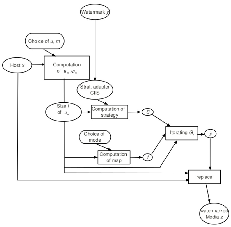
Figure 1: The dhCI dissimulation scheme

Next section shows how to check whether a media contains a watermark.

2.3 Decoding

Let us firstly show how to formally check whether a given digital media $z$ results from the dissimulation of $y$ into the digital media $x$.

Definition 10 (Watermarked content)

Let $\textit{dec}(u,m,M)$ be a decomposition function, $f$ be a mode, $\mathcal{S}$ be a strategy adapter, $q$ be a positive natural number, $y$ be a digital media, and $(u_{M},u_{m},u_{p},\phi_{M},\phi_{m},\phi_{p})$ be the image by $\textit{dec}(u,m,M)$ of a digital media $x$. Then $z$ is watermarked with $y$ if the image by $\textit{dec}(u,m,M)$ of $z$ is $(u_{M},u_{m},u_{p},\phi_{M},\hat{y},\phi_{p})$, where $\hat{y}$ is the right member of $G_{f_{l}}^{q}(S_{y},\phi_{m})$. _□

Various decision strategies are obviously possible to determine whether a given image $z$ is watermarked or not, depending on the eventuality that the considered image may have been attacked. For example, a similarity percentage between $x$ and $z$ can be computed and compared to a given threshold. Other possibilities are the use of ROC curves or the definition of a null hypothesis problem.

The next section recalls some security properties and shows how the dhCI dissimulation algorithm verifies them.

3 Security analysis

3.1 State-of-the-art in information hiding security

As far as we know, Cachin [15] produces the first fundamental work in information hiding security: in the context of steganography, the attempt of an attacker to distinguish between an innocent image and a stego-content is viewed as an hypothesis testing problem. Mittelholzer [16] next proposed the first theoretical framework for analyzing the security of a watermarking scheme. Clarification between robustness and security and classifications of watermarking attacks have been firstly presented by Kalker [17]. This work has been deepened by Furon et al. [18], who have translated Kerckhoffs’ principle (Alice and Bob shall only rely on some previously shared secret for privacy), from cryptography to data hiding.

More recently [19, 20] classified the information hiding attacks into categories, according to the type of information the attacker (Eve) has access to:

• in Watermarked Only Attack (WOA) she only knows embedded contents $z$;

• in Known Message Attack (KMA) she knows pairs $(z,y)$ of embedded contents and corresponding messages;

• in Known Original Attack (KOA) she knows several pairs $(z,x)$ of embedded contents and their corresponding original versions;

• in Constant-Message Attack (CMA) she observes several embedded contents $z^{1}$,…,$z^{k}$ and only knows that the unknown hidden message $y$ is the same in all contents.

To the best of our knowledge, KMA, KOA, and CMA have not already been studied due to the lack of theoretical framework. In the opposite, security of data hiding against WOA can be evaluated, by using a probabilistic approach recalled below.

3.2 Stego-security

In the Simmons’ prisoner problem [21], Alice and Bob are in jail and they want to, possibly, devise an escape plan by exchanging hidden messages in innocent-looking cover contents. These messages are to be conveyed to one another by a common warden named Eve, who eavesdrops all contents and can choose to interrupt the communication if they appear to be stego-contents.

Stego-security, defined in this well-known context, is the highest security class in Watermark-Only Attack setup, which occurs when Eve has only access to several marked contents [8].

Let $\mathds{K}$ be the set of embedding keys, $p(X)$ the probabilistic model of $N_{0}$ initial host contents, and $p(Y|K)$ the probabilistic model of $N_{0}$ marked contents s.t. each host content has been marked with the same key $K$ and the same embedding function.

Definition 11 (Stego-Security [8])

The embedding function is stego-secure if $\forall K\in\mathds{K},p(Y|K)=p(X)$ is established. _□

Stego-security states that the knowledge of $K$ does not help to make the difference between $p(X)$ and $p(Y)$. This definition implies the following property:

$$p(Y|K_{1})=\cdots=p(Y|K_{N_{k}})=p(Y)=p(X)$$

This property is equivalent to a zero Kullback-Leibler divergence, which is the accepted definition of the ”perfect secrecy” in steganography [15].

3.3 The negation mode is stego-secure

To make this article self-contained, this section recalls theorems and proofs of stego-security for negation mode published in [10].

Proposition 1

dhCI dissimulation of Definition 9 with negation mode and CIIS strategy-adapter is stego-secure, whereas it is not the case when using CIDS strategy-adapter. _□

Proof

On the one hand, let us suppose that $X\sim\mathbf{U}\left(\mathbb{B}^{n}\right)$ when using CIIS$(K,\_,\_,l)$. We prove by a mathematical induction that $\forall t\in\mathds{N},X^{t}\sim\mathbf{U}\left(\mathbb{B}^{n}\right)$.

The base case is immediate, as $X^{0}=X\sim\mathbf{U}\left(\mathbb{B}^{n}\right)$. Let us now suppose that the statement $X^{t}\sim\mathbf{U}\left(\mathbb{B}^{n}\right)$ holds until for some $t$. Let $e\in\mathbb{B}^{n}$ and $\mathbf{B}_{k}=(0,\cdots,0,1,0,\cdots,0)\in\mathbb{B}^{n}$ (the digit $1$ is in position $k$).

So $P\left(X^{t+1}=e\right)=\sum_{k=1}^{n}P\left(X^{t}=e\oplus\mathbf{B}_{k},S^{t}=k\right)$ where $\oplus$ is again the bitwise exclusive or. These two events are independent when using CIIS strategy-adapter (contrary to CIDS, CIIS is not built by using $X$), thus:

$$P\left(X^{t+1}=e\right)=\sum_{k=1}^{n}P\left(X^{t}=e\oplus\mathbf{B}_{k}\right)\times P\left(S^{t}=k\right).$$

According to the inductive hypothesis: $P\left(X^{n+1}=e\right)=\frac{1}{2^{n}}\sum_{k=1}^{n}P\left(S^{t}=k\right)$. The set of events $\left\{S^{t}=k\right\}$ for $k\in\llbracket 1;n\rrbracket$ is a partition of the universe of possible, so $\sum_{k=1}^{n}P\left(S^{t}=k\right)=1$. Finally, $P\left(X^{t+1}=e\right)=\frac{1}{2^{n}}$, which leads to $X^{t+1}\sim\mathbf{U}\left(\mathbb{B}^{n}\right)$. This result is true for all $t\in\mathds{N}$ and then for $t=l$.

Since $P(Y|K)$ is $P(X^{l})$ that is proven to be equal to $P(X)$, we thus have established that,

$$\forall K\in[0;1],P(Y|K)=P(X^{l})=P(X).$$

So dhCI dissimulation with CIIS strategy-adapter is stego-secure.

On the other hand, due to the definition of CIDS, we have $P(Y=(1,1,\cdots,1)|K)=0$. So there is no uniform repartition for the stego-contents $Y|K$. _■

To sum up, Alice and Bob can counteract Eve’s attacks in WOA setup, when using dhCI dissimulation with CIIS strategy-adapter. To our best knowledge, this is the second time an information hiding scheme has been proven to be stego-secure: the former was the spread-spectrum technique in natural marking configuration with $\eta$ parameter equal to 1 [8].

3.4 A new class of $\varepsilon$-stego-secure schemes

Let us prove that,

Theorem 1

Let $\epsilon$ be positive, $l$ be any size of LSCs, $X\sim\mathbf{U}\left(\mathbb{B}^{l}\right)$, $f_{l}$ be an image mode s.t. $\Gamma(f_{l})$ is strongly connected and the Markov matrix associated to $f_{l}$ is doubly stochastic. In the instantiated dhCI dissimulation algorithm with any uniformly distributed (u.d.) strategy-adapter that is independent from $X$, there exists some positive natural number $q$ s.t. $|p(X^{q})-p(X)|<\epsilon$. _□

Proof

Let deci be the bijection between $\mathds{B}^{l}$ and $\llbracket 0,2^{l}-1\rrbracket$ that associates the decimal value of any binary number in $\mathds{B}^{l}$. The probability $p(X^{t})=(p(X^{t}=e_{0}),\dots,p(X^{t}=e_{2^{l}-1}))$ for $e_{j}\in\mathds{B}^{l}$ is thus equal to $(p(\textit{deci}(X^{t})=0,\dots,p(\textit{deci}(X^{t})=2^{l}-1))$ further denoted by $\pi^{t}$. Let $i\in\llbracket 0,2^{l}-1\rrbracket$, the probability $p(\textit{deci}(X^{t+1})=i)$ is

$$\sum\limits^{2^{l}-1}_{j=0}\sum\limits^{l}_{k=1}p(\textit{deci}(X^{t})=j,S^{t}=k,i=_{k}j,f_{k}(j)=i_{k})$$

where $i=_{k}j$ is true iff the binary representations of $i$ and $j$ may only differ for the $k$-th element, and where $i_{k}$ abusively denotes, in this proof, the $k$-th element of the binary representation of $i$.

Next, due to the proposition’s hypotheses on the strategy, $p(\textit{deci}(X^{t})=j,S^{t}=k,i=_{k}j,f_{k}(j)=i_{k})$ is equal to $\frac{1}{l}.p(\textit{deci}(X^{t})=j,i=_{k}j,f_{k}(j)=i_{k})$. Finally, since $i=_{k}j$ and $f_{k}(j)=i_{k}$ are constant during the iterative process and thus does not depend on $X^{t}$, we have

$$\pi^{t+1}_{i}=\sum\limits^{2^{l}-1}_{j=0}\pi^{t}_{j}.\frac{1}{l}\sum\limits^{l}_{k=1}p(i=_{k}j,f_{k}(j)=i_{k}).$$

Since $\frac{1}{l}\sum\limits^{l}_{k=1}p(i=_{k}j,f_{k}(j)=i_{k})$ is equal to $M_{ji}$ where $M$ is the Markov matrix associated to $f_{l}$ we thus have

$$\pi^{t+1}_{i}=\sum\limits^{2^{l}-1}_{j=0}\pi^{t}_{j}.M_{ji}\textrm{ and thus }\pi^{t+1}=\pi^{t}M.$$

First of all, since the graph $\Gamma(f)$ is strongly connected, then for all vertices $i$ and $j$, a path can be found to reach $j$ from $i$ in at most $2^{l}$ steps. There exists thus $k_{ij}\in\llbracket 1,2^{l}\rrbracket$ s.t. ${M}_{ij}^{k_{ij}}>0$. As all the multiples $l\times k_{ij}$ of $k_{ij}$ are such that ${M}_{ij}^{l\times k_{ij}}>0$, we can conclude that, if $k$ is the least common multiple of $\{k_{ij}\big{/}i,j\in\llbracket 1,2^{l}\rrbracket\}$ thus $\forall i,j\in\llbracket 1,2^{l}\rrbracket,{M}_{ij}^{k}>0$ and thus $M$ is a regular stochastic matrix.

Let us now recall the following stochastic matrix theorem:

Theorem 2 (Stochastic Matrix)

If $M$ is a regular stochastic matrix, then $M$ has an unique stationary probability vector $\pi$. Moreover, if $\pi^{0}$ is any initial probability vector and $\pi^{t+1}=\pi^{t}.M$ for $t=0,1,\dots$ then the Markov chain $\pi^{t}$ converges to $\pi$ as $t$ tends to infinity. _□

Thanks to this theorem, $M$ has an unique stationary probability vector $\pi$. By hypothesis, since $M$ is doubly stochastic we have $(\frac{1}{2^{l}},\dots,\frac{1}{2^{l}})=(\frac{1}{2^{l}},\dots,\frac{1}{2^{l}})M$ and thus $\pi=(\frac{1}{2^{l}},\dots,\frac{1}{2^{l}})$. Due to the matrix theorem, there exists some $q$ s.t. $|\pi^{q}-\pi|<\epsilon$ and the proof is established. Since $p(Y|K)$ is $p(X^{q})$ the method is then $\epsilon$-stego-secure provided the strategy-adapter is uniformly distributed. _■

This section has focused on security with regards to probabilistic behaviors. Next section studies it in the perspective of topological ones.

4 Chaos-security

To check whether an existing data hiding scheme is chaotic or not, we propose firstly to write it as an iterate process $x^{n+1}=f(x^{n})$. It is possible to prove that this formulation can always be done, as follows. Let us consider a given data hiding algorithm. Because it must be computed one day, it is always possible to translate it as a Turing machine, and this last machine can be written as $x^{n+1}=f(x^{n})$ in the following way. Let $(w,i,q)$ be the current configuration of the Turing machine (Fig. 2), where $w=\sharp^{-\omega}w(0)\ldots w(k)\sharp^{\omega}$ is the paper tape, $i$ is the position of the tape head, $q$ is used for the state of the machine, and $\delta$ is its transition function (the notations used here are well-known and widely used). We define $f$ by:

• $f(w(0)\ldots w(k),i,q)=(w(0)\ldots w(i-1)aw(i+1)w(k),i+1,q^{\prime})$, if $\delta(q,w(i))=(q^{\prime},a,\rightarrow)$;

• $f(w(0)\ldots w(k),i,q)=(w(0)\ldots w(i-1)aw(i+1)w(k),i-1,q^{\prime})$, if $\delta(q,w(i))=(q^{\prime},a,\leftarrow)$.

Thus the Turing machine can be written as an iterate function $x^{n+1}=f(x^{n})$ on a well-defined set $\mathcal{X}$, with $x^{0}$ as the initial configuration of the machine. We denote by $\mathcal{T}(S)$ the iterative process of a data hiding scheme $S$.

Figure 2: Turing Machine

Let us now define the notion of chaos-security. Let $\tau$ be a topology on $\mathcal{X}$. So the behavior of this dynamical system can be studied to know whether or not the data hiding scheme is $\tau-$unpredictable. This leads to the following definition.

Definition 12

An information hiding scheme $S$ is said to be chaos-secure on $(\mathcal{X},\tau)$ if its iterative process $\mathcal{T}(S)$ has a chaotic behavior, as defined by Devaney, on this topological space. _□

Theoretically speaking, chaos-security can always be studied, as it only requires that the two following points are satisfied.

• Firstly, the data hiding scheme must be written as an iterate function on a set $\mathcal{X}$; As illustrated by the use of the Turing machine, it is always possible to satisfy this requirement; It is established here since we iterate $G_{f}$ as defined in Sect. (2.1);

• Secondly, a metric or a topology must be defined on $\mathcal{X}$; This is always possible, for example, by taking for instance the most relevant one, that is the order topology.

Guyeux has recently shown in [11] that chaotic iterations of $G_{f}$ with the vectorial negation as iterate function have a chaotic behavior. As a corollary, we deduce that the dhCI dissimulation algorithm with negation mode and CIIS strategy-adapter is chaos-secure.

However, all these results suffer from only relying on the vectorial negation function. This problem has been theoretically tackled in [11] which provides the following theorem.

Theorem 3

Functions $f:\mathds{B}^{n}\to\mathds{B}^{n}$ such that $G_{f}$ is chaotic according to Devaney, are functions such that the graph $\Gamma(f)$ is strongly connected. _□

We deduce from this theorem that functions whose graph is strongly connected are sufficient to provide new instances of dhCI dissimulation that are chaos-secure.

Computing a mode $f$ such that the image of $n$ (i.e., $f_{n}$) is a function with a strongly connected graph of iterations $\Gamma(f_{n})$ has been previously studied (see [22] for instance). The next section presents a use of them in our steganography context.

5 Applications to frequential domains

We are then left to provide an u.d. strategy-adapter that is independent from the cover, an image mode $f_{l}$ whose iteration graph $\Gamma(f_{l})$ is strongly connected and whose Markov matrix is doubly stochastic.

First, the $\textit{CIIS}(K,y,\alpha,l)$ strategy adapter (see Section 2.2) has the required properties: it does not depend on the cover and the proof that its outputs are u.d. on $\llbracket 1;l\rrbracket$ is left as an exercise for the reader. In all the experiments parameters $K$ and $\alpha$ are randomly chosen in $\rrbracket 0,1\llbracket$ and $\rrbracket 0,0.5\llbracket$ respectively. The number of iteration is set to $4*lm$, where $lm$ is the number of LSCs that depends on the domain.

Next, [22] has presented an iterative approach to generate image modes $f_{l}$ such that $\Gamma(f_{l})$ is strongly connected. Among these maps, it is obvious to check which verifies or not the doubly stochastic constrain. For instance, in what follows we consider the mode $f_{l}:\mathds{B}^{l}\rightarrow\mathds{B}^{l}$ s.t. its $i$th component is defined by

$${f_{l}}(x)_{i}=\left\{\begin{array}[]{l}\overline{x_{i}}\textrm{ if $i$ is odd}\\ x_{i}\oplus x_{i-1}\textrm{ if $i$ is even}\end{array}\right.$$ (1)

Thanks to [22, Theorem 2] we deduce that its iteration graph $\Gamma(f_{l})$ is strongly connected. Next, the Markov chain is stochastic by construction.

Let us prove that its Markov chain is doubly stochastic by induction on the length $l$. For $l=1$ and $l=2$ the proof is obvious. Let us consider that the result is established until $l=2k$ for some $k\in\mathbb{N}$.

Let us then firstly prove the doubly stochasticity for $l=2k+1$. Following notations introduced in [22], let $\Gamma(f_{2k+1})^{0}$ and $\Gamma(f_{2k+1})^{1}$ denote the subgraphs of $\Gamma(f_{2k+1})$ induced by the subset $\mathds{B}^{2k}\times\{0\}$ and $\mathds{B}^{2k}\times\{1\}$ of $\mathds{B}^{2k+1}$ respectively. $\Gamma(f_{2k+1})^{0}$ and $\Gamma(f_{2k+1})^{1}$ are isomorphic to $\Gamma(f_{2k})$. Furthermore, these two graphs are linked together only with arcs of the form $(x_{1},\dots,x_{2k},0)\to(x_{1},\dots,x_{2k},1)$ and $(x_{1},\dots,x_{2k},1)\to(x_{1},\dots,x_{2k},0)$. In $\Gamma(f_{2k+1})$ the number of arcs whose extremity is $(x_{1},\dots,x_{2k},0)$ is the same than the number of arcs whose extremity is $(x_{1},\dots,x_{2k})$ augmented with 1, and similarly for $(x_{1},\dots,x_{2k},1)$. By induction hypothesis, the Markov chain associated to $\Gamma(f_{2k})$ is doubly stochastic. All the vertices $(x_{1},\dots,x_{2k})$ have thus the same number of ingoing arcs and the proof is established for $l$ is $2k+1$.

Let us then prove the doubly stochasticity for $l=2k+2$. The map $f_{l}$ is defined by $f_{l}(x)=(\overline{x_{1}},x_{2}\oplus x_{1},\dots,\overline{x_{2k+1}},x_{2k+2}\oplus x_{2k+1})$. With previously defined notations, let us focus on $\Gamma(f_{2k+2})^{0}$ and $\Gamma(f_{2k+2})^{1}$ which are isomorphic to $\Gamma(f_{2k+1})$. Among configurations of $\mathds{B}^{2k+2}$, only four suffixes of length 2 can be obviously observed, namely, $00$, $10$, $11$ and $01$. Since $f_{2k+2}(\dots,0,0)_{2k+2}=0$, $f_{2k+2}(\dots,1,0)_{2k+2}=1$, $f_{2k+2}(\dots,1,1)_{2k+2}=0$, and $f_{2k+2}(\dots,0,1)_{2k+2}=1$, the number of arcs whose extremity is

• $(x_{1},\dots,x_{2k},0,0)$ is the same than the one whose extremity is $(x_{1},\dots,x_{2k},0)$ in $\Gamma(f_{2k+1})$ augmented with 1 (loop over configurations $(x_{1},\dots,x_{2k},0,0)$);

• $(x_{1},\dots,x_{2k},1,0)$ is the same than the one whose extremity is $(x_{1},\dots,x_{2k},0)$ in $\Gamma(f_{2k+1})$ augmented with 1 (arc from configurations $(x_{1},\dots,x_{2k},1,1)$ to configurations $(x_{1},\dots,x_{2k},1,0)$);

• $(x_{1},\dots,x_{2k},0,1)$ is the same than the one whose extremity is $(x_{1},\dots,x_{2k},0)$ in $\Gamma(f_{2k+1})$ augmented with 1 (loop over configurations $(x_{1},\dots,x_{2k},0,1)$);

• $(x_{1},\dots,x_{2k},1,1)$ is the same than the one whose extremity is $(x_{1},\dots,x_{2k},1)$ in $\Gamma(f_{2k+1})$ augmented with 1 (arc from configurations $(x_{1},\dots,x_{2k},1,0)$ to configurations $(x_{1},\dots,x_{2k},1,1)$).

Thus all the vertices $(x_{1},\dots,x_{2k})$ have the same number of ingoing arcs and the proof is established for $l=2k+2$.

5.1 DWT embedding

Let us now explain how the dhCI dissimulation can be applied in the discrete wavelets domain (DWT). In this paper, the Daubechies family of wavelets is chosen: each DWT decomposition depends on a decomposition level and a coefficient matrix (Figure 3): LL means approximation coefficient, when $\textit{HH},\textit{LH},\textit{HL}$ denote respectively diagonal, vertical, and horizontal detail coefficients. For example, the DWT coefficient HH2 is the matrix equal to the diagonal detail coefficient of the second level of decomposition of the image.

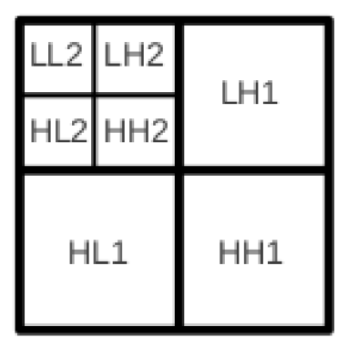
Figure 3: Wavelets coefficients.

The choice of the detail level is motivated by finding a good compromise between robustness and invisibility. Choosing low or high frequencies in DWT domain leads either to a very fragile watermarking without robustness (especially when facing a JPEG2000 compression attack) or to a large degradation of the host content. In order to have a robust but discrete DWT embedding, the second detail level (i.e., $\textit{LH}2,\textit{HL}2,\textit{HH}2$) that corresponds to the middle frequencies, has been retained.

Let us consider the Daubechies wavelet coefficients of a third level decomposition as represented in Figure 3. We then translate these float coefficients into their 32-bits values. Let us define the significance function $u$ that associates to any index $k$ in this sequence of bits the following numbers:

• $u^{k}=-1$ if $k$ is one of the three last bits of any index of coefficients in $\textit{LH}2$, $\textit{HL}2$, or in $\textit{HH}2$;

• $u^{k}=0$ if $k$ is an index of a coefficient in $\textit{LH}1$, $\textit{HL}1$, or in $\textit{HH}1$;

• $u^{k}=1$ otherwise.

According to the definition of significance of coefficients (Def. 5), if $(m,M)$ is $(-0.5,0.5)$, LSCs are the last three bits of coefficients in $\textit{HL}2$,$\textit{HH}2$, and $\textit{LH}2$. Thus, decomposition and recomposition functions are fully defined and dhCI dissimulation scheme can now be applied.

Figure 4 shows the result of a dhCI dissimulation embedding into DWT domain. The original is the image 5007 of the BOSS contest [23]. Watermark $y$ is given in Fig. 4(b).

From a random selection of 50 images into the database from the BOSS contest [23], we have applied the previous algorithm with mode $f_{l}$ defined in Equation (1) and with the negation mode.

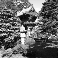
(a) Original Image.

(b) Watermark $y$.

(c) Watermarked Image.

Figure 4: Data hiding in DWT domain

5.2 DCT embedding

Let us denote by $x$ the original image of size $H\times L$, and by $y$ the hidden message, supposed here to be a binary image of size $H^{\prime}\times L^{\prime}$. The image $x$ is transformed from the spatial domain to DCT domain frequency bands, in order to embed $y$ inside it. To do so, the host image is firstly divided into $8\times 8$ image blocks as given below:

$$x=\bigcup_{k=1}^{H/8}\bigcup_{k^{\prime}=1}^{L/8}x(k,k^{\prime}).$$

Thus, for each image block, a DCT is performed and the coefficients in the frequency bands are obtained as follows: $x_{DCT}(m;n)=DCT(x(m;n))$.

To define a discrete but robust scheme, only the four following coefficients of each $8\times 8$ block in position $(m,n)$ will be possibly modified: $x_{DCT}(m;n)_{(3,1)},$ $x_{DCT}(m;n)_{(2,2)},$ or $x_{DCT}(m;n)_{(1,3)}$. This choice can be reformulated as follows. Coefficients of each DCT matrix are re-indexed by using a southwest/northeast diagonal, such that $i_{DCT}(m,n)_{1}=x_{DCT}(m;n)_{(1,1)}$,$i_{DCT}(m,n)_{2}=x_{DCT}(m;n)_{(2,1)}$, $i_{DCT}(m,n)_{3}=x_{DCT}(m;n)_{(1,2)}$, $i_{DCT}(m,n)_{4}=x_{DCT}(m;n)_{(3,1)}$, …, and $i_{DCT}(m,n)_{64}=$ $x_{DCT}(m;n)_{(8,8)}$. So the signification function can be defined in this context by:

• if $k$ mod $64\in\{1,2,3\}$ and $k\leqslant H\times L$, then $u^{k}=1$;

• else if $k$ mod $64\in\{4,5,6\}$ and $k\leqslant H\times L$, then $u^{k}=-1$;

• else $u^{k}=0$.

The significance of coefficients are obtained for instance with $(m,M)=(-0.5,0.5)$ leading to the definitions of MSCs, LSCs, and passive coefficients. Thus, decomposition and recomposition functions are fully defined and dhCI dissimulation scheme can now be applied.

5.3 Image quality

This section focuses on measuring visual quality of our steganographic method. Traditionally, this is achieved by quantifying the similarity between the modified image and its reference image. The Mean Squared Error (MSE) and the Peak Signal to Noise Ratio (PSNR) are the most widely known tools that provide such a metric. However, both of them do not take into account Human Visual System (HVS) properties. Recent works [24, 25, 26, 27] have tackled this problem by creating new metrics. Among them, what follows focuses on PSNR-HVS-M [26] and BIQI [27], considered as advanced visual quality metrics. The former efficiently combines PSNR and visual between-coefficient contrast masking of DCT basis functions based on HVS. This metric has been computed here by using the implementation given at [28]. The latter allows to get a blind image quality assessment measure, i.e., without any knowledge of the source distortion. Its implementation is available at [29].

Embedding	DWT		DCT
Mode	$f_{l}$	neg.	$f_{l}$	neg.
PSNR	42.74	42.76	52.68	52.41
PSNR-HVS-M	44.28	43.97	45.30	44.93
BIQI	35.35	32.78	41.59	47.47

Table 1: Quality measeures of our steganography approach

Results of the image quality metrics are summarized into the Table 1. In wavelet domain, the PSNR values obtained here are comparable to other approaches (for instance, PSNR are 44.2 in [30] and 46.5 in [31]), but a real improvement for the discrete cosine embeddings is obtained (PSNR is 45.17 for [32], it is always lower than 48 for [33], and always lower than 39 for [34]). Among steganography approaches that evaluate PSNR-HVS-M, results of our approach are convincing. Firstly, optimized method developed along [35] has a PSNR-HVS-M equal to 44.5 whereas our approach, with a similar PSNR-HVS-M, should be easily improved by considering optimized mode. Next, another approach [36] have higher PSNR-HVS-M, certainly, but this work does not address robustness evaluation whereas our approach is complete. Finally, as far as we know, this work is the first one that evaluates the BIQI metric in the steganography context.

With all this material, we are then left to evaluate the robustness of this approach.

5.4 Robustness

Previous sections have formalized frequential domains embeddings and has focused on the negation mode and $f_{l}$ defined in Equ. (1). In the robustness given in this continuation, dwt(neg), dwt(fl), dct(neg), dct(fl) respectively stand for the DWT and DCT embedding with the negation mode and with this instantiated mode.

For each experiment, a set of 50 images is randomly extracted from the database taken from the BOSS contest [23]. Each cover is a $512\times 512$ grayscale digital image and the watermark $y$ is given in Fig 4(b). Testing the robustness of the approach is achieved by successively applying on watermarked images attacks like cropping, compression, and geometric transformations. Differences between $\hat{y}$ and $\varphi_{m}(z)$ are computed. Behind a given threshold rate, the image is said to be watermarked. Finally, discussion on metric quality of the approach is given in Sect. 5.5.

Robustness of the approach is evaluated by applying different percentage of cropping: from 1% to 81%. Results are presented in Fig. 5. Fig. 5(a) gives the cropped image where 36% of the image is removed. Fig. 5(b) presents effects of such an attack. From this experiment, one can conclude that all embeddings have similar behaviors. All the percentage differences are so far less than 50% (which is the mean random error) and thus robustness is established.

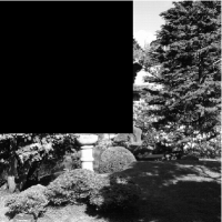
(a) Cropped Image.

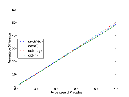
(b) Cropping Effect

Figure 5: Cropping Results

5.4.1 Robustness against compression

Robustness against compression is addressed by studying both JPEG and JPEG 2000 image compressions. Results are respectively presented in Fig. 6(a) and Fig. 6(b). Without surprise, DCT embedding which is based on DCT (as JPEG compression algorithm is) is more adapted to JPEG compression than DWT embedding. Furthermore, we have a similar behavior for the JPEG 2000 compression algorithm, which is based on wavelet encoding: DWT embedding naturally outperforms DCT one in that case.

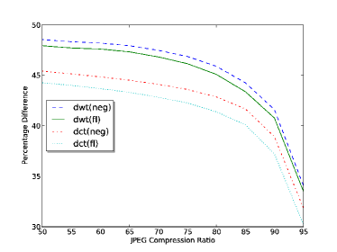
(a) JPEG Effect

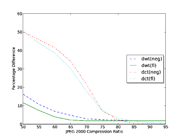
(b) JPEG 2000 Effect

Figure 6: Compression Results

5.4.2 Robustness against Contrast and Sharpness Attack

Contrast and Sharpness adjustment belong to the the classical set of filtering image attacks. Results of such attacks are presented in Fig. 7 where Fig. 7(a) and Fig. 7(b) summarize effects of contrast and sharpness adjustment respectively.

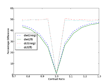
(a) Contrast Effect

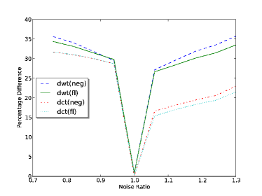
(b) Sharpness Effect

Figure 7: Filtering Results

5.4.3 Robustness against Geometric Transformation

Among geometric transformations, we focus on rotations, i.e., when two opposite rotations of angle $\theta$ are successively applied around the center of the image. In these geometric transformations, angles range from 2 to 20 degrees. Results are presented in Fig. 8: Fig. 8(a) gives the image of a rotation of 20 degrees whereas Fig. 8(b) presents effects of such an attack. It is not a surprise that results are better for DCT embeddings: this approach is based on cosine as rotation is.

(a) 20 degrees Rotation Image

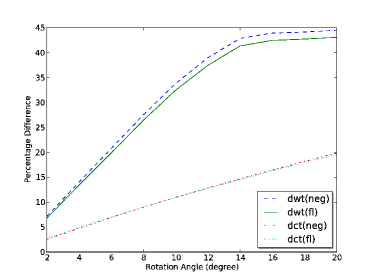
(b) Rotation Effect

Figure 8: Rotation Attack Results

5.5 Evaluation of the Embeddings

We are then left to set a convenient threshold that is accurate to determine whether an image is watermarked or not. Starting from a set of 100 images selected among the Boss image Panel, we compute the following three sets: the one with all the watermarked images $W$, the one with all successively watermarked and attacked images WA, and the one with only the attacked images $A$. Notice that the 100 attacks for each images are selected among these detailed previously.

For each threshold $t\in\llbracket 0,55\rrbracket$ and a given image $x\in\textit{WA}\cup A$, differences on DCT are computed. The image is said to be watermarked if these differences are less than the threshold. In the positive case and if $x$ really belongs to WA it is a True Positive (TP) case. In the negative case but if $x$ belongs to WA it is a False Negative (FN) case. In the positive case but if $x$ belongs to A, it is a False Positive (FP) case. Finally, in the negative case and if $x$ belongs to A, it is a True Negative (TN). The True (resp. False) Positive Rate (TPR) (resp. FPR) is thus computed by dividing the number of TP (resp. FP) by 100.

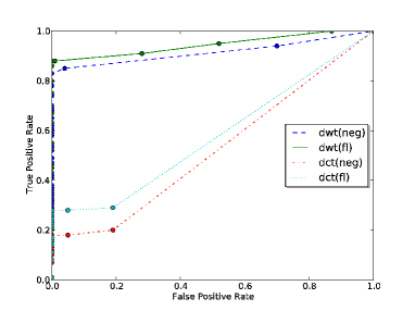
Figure 9: ROC Curves for DWT or DCT Embeddings

The Figure 9 is the Receiver Operating Characteristic (ROC) curve. For the DWT, it shows that best results are obtained when the threshold is 45% for the dedicated function (corresponding to the point (0.01, 0.88)) and 46% for the negation function (corresponding to the point (0.04, 0.85)). It allows to conclude that each time LSCs differences between a watermarked image and another given image $i^{\prime}$ are less than 45%, we can claim that $i^{\prime}$ is an attacked version of the original watermarked content. For the two DCT embeddings, best results are obtained when the threshold is 44% (corresponding to the points (0.05, 0.18) and (0.05, 0.28)).

Let us then give some confidence intervals for all the evaluated attacks. The approach is resistant to:

• all the croppings where percentage is less than 85;

• compressions where quality ratio is greater than 82 with DWT embedding and where quality ratio is greater than 67 with DCT one;

• contrast when strengthening belongs to $[0.76,1.2]$ (resp. $[0.96,1.05]$) in DWT (resp. in DCT) embedding;

• all the rotation attacks with DCT embedding and a rotation where angle is less than 13 degrees with DWT one.

6 Conclusion

This paper has proposed a new class of secure and robust information hiding algorithms. It has been entirely formalized, thus allowing both its theoretical security analysis, and the computation of numerous variants encompassing spatial and frequency domain embedding. After having presented the general algorithm with detail, we have given conditions for choosing mode and strategy-adapter making the whole class stego-secure or $\epsilon$-stego-secure. To our knowledge, this is the first time such a result has been established.

Applications in frequency domains (namely DWT and DCT domains) have finally be formalized. Complete experiments have allowed us first to evaluate how invisible is the steganographic method (thanks to the PSNR computation) and next to verify the robustness property against attacks. Furthermore, the use of ROC curves for DWT embedding have revealed very high rates between True positive and False positive results.

In future work, our intention is to find the best image mode with respect to the combination between DCT and DWT based steganography algorithm. Such a combination topic has already been addressed (e.g., in [37]), but never with objectives we have set.

Additionally, we will try to discover new topological properties for the dhCI dissimulation schemes. Consequences of these chaos properties will be drawn in the context of information hiding security. We will especially focus on the links between topological properties and classes of attacks, such as KOA, KMA, EOA, or CMA.

Moreover, these algorithms will be compared to other existing ones, among other things by testing whether these algorithms are chaotic or not. Finally we plan to verify the robustness of our approach against statistical steganalysis methods [38, 39, 40, 41].

References

- [1] Houmansadr, A., Kiyavash, N., and Borisov, N. (2009) Rainbow: A robust and invisible non-blind watermark for network flows. Proceedings of the Network and Distributed System Security Symposium, NDSS 2009,San Diego, February. The Internet Society, Washington DC/Reston.
- [2] G.S.El-Taweel, Onsi, H., M.Samy, and Darwish, M. (2005) Secure and non-blind watermarking scheme for color images based on dwt. ICGST International Journal on Graphics, Vision and Image Processing, 05, 1–5.
- [3] Wu, X., Guan, Z.-H., and Wu, Z. (2007) A chaos based robust spatial domain watermarking algorithm. ISNN ’07: Proceedings of the 4th international symposium on Neural Networks, Nanjing, China, Berlin, June, Lecture Notes in Computer Science, 4492, pp. 113–119. Springer-Verlag.
- [4] Liu, Z. and Xi, L. (2007) Image information hiding encryption using chaotic sequence. Knowledge-Based Intelligent Information and Engineering Systems, 11th International Conference, KES 2007, XVII Italian Workshop on Neural Networks, Vietri sul Mare, Italy, Berlin, September, pp. 202–208. Springer-Verlag.
- [5] Cong, J., Jiang, Y., Qu, Z., and Zhang, Z. (2006) A wavelet packets watermarking algorithm based on chaos encryption. Computational Science and Its Applications - ICCSA 2006, International Conference, Glasgow, UK, Berlin, May, Lecture Notes in Computer Science, 3980, pp. 921–928. Springer-Verlag.
- [6] Congxu, Z., Xuefeng, L., and Zhihua, L. (2006) Chaos-based multipurpose image watermarking algorithm. Wuhan University Journal of Natural Sciences, 11, 1675–1678.
- [7] Wu, X. and Guan, Z.-H. (2007) A novel digital watermark algorithm based on chaotic maps. Physics Letters A, 365, 403 – 406.
- [8] Cayre, F. and Bas, P. (2008) Kerckhoffs-based embedding security classes for woa data hiding. IEEE Transactions on Information Forensics and Security, 3, 1–15.
- [9] Cox, I. J., Member, S., Kilian, J., Leighton, F. T., and Shamoon, T. (1997) Secure spread spectrum watermarking for multimedia. IEEE Transactions on Image Processing, 6, 1673–1687.
- [10] Guyeux, C., Friot, N., and Bahi, J. (2010) Chaotic iterations versus spread-spectrum: chaos and stego security. Sixth International Conference on Intelligent Information Hiding and Multimedia Signal Processing (IIH-MSP 2010), Darmstadt, Germany, Washington, DC, October, pp. 208–211. IEEE Computer Society.
- [11] Guyeux, C. (2010) Le désordre des itérations chaotiques et leur utilité en s curité informatique. PhD thesis Université de Franche-Comté.
- [12] Devaney, R. L. (2003) An Introduction to Chaotic Dynamical Systems, 2nd Edition. Westview Press, Boulder, CO.
- [13] Shujun, L., Qi, L., Wenmin, L., Xuanqin, M., and Yuanlong, C. (2001) Statistical properties of digital piecewise linear chaotic maps and their roles in cryptography and pseudo-random coding. Cryptography and Coding, 8th IMA International Conference, Cirencester, UK, Berlin, December, Lecture Notes in Computer Science, 2260, pp. 205–221. Springer-Verlag.
- [14] Arroyo, D., Alvarez, G., and Fernandez, V. (2008) On the inadequacy of the logistic map for cryptographic applications. arXiv/0805.4355.
- [15] Cachin, C. (1998) An information-theoretic model for steganography. Information Hiding, Second International Workshop, Portland, Oregon, USA, Berlin, April, Lecture Notes in Computer Science, 1525, pp. 306–318. Springer-Verlag.
- [16] Mittelholzer, T. (1999) An information-theoretic approach to steganography and watermarking. nformation Hiding, Third International Workshop, IH’99, Dresden, Germany, Berlin, September, pp. 1–16. Springer-Verlag.
- [17] Kalker, T. (2001) Considerations on watermarking security. 2001 IEEE Fourth Workshop on Multimedia Signal Processing, Cannes, France, Washington, DC, October, pp. 201–206. IEEE Computer Society.
- [18] Furon, T. (2002). Security analysis. European Project IST-1999-10987 CERTIMARK, Deliverable D.5.5.
- [19] Cayre, F., Fontaine, C., and Furon, T. (2005) Watermarking security: theory and practice. IEEE Transactions on Signal Processing, 53, 3976–3987.
- [20] Perez-Freire, L., P rez-Gonzalez, F., and Comesa a, P. (2006) Secret dither estimation in lattice-quantization data hiding: A set-membership approach. Security, Steganography, and Watermarking of Multimedia Contents, San Jose, California, Bellingham, WA, January, pp. 1–12. Society of Photo-Optical Instrumentation Engineers.
- [21] Simmons, G. J. (1984) The prisoners’ problem and the subliminal channel. Advances in Cryptology, Proc. CRYPTO’83, University of California, Santa Barbara, New York, August, pp. 51–67. Plenum Press.
- [22] Bahi, J., Couchot, J.-F., Guyeux, C., and Richard, A. (2011) On the link between strongly connected iteration graphs and chaotic boolean discrete-time dynamical systems. FCT’11, 18th Int. Symp. on Fundamentals of Computation Theory,Oslo, Norway, Berlin, August, Lecture Notes in Computer Science, 6914, pp. 126–137. Springer-Verlag.
- [23] Pevný, T., Filler, T., and Bas, P. (2010). Break our steganographic system. available at http://www.agents.cz/boss/.
- [24] Egiazarian, K., Astola, J., Ponomarenko, V., Nikolayand Lukin, Battisti, F., and Carli, M. (2006) New full-reference quality metrics based on hvs. In Li, B. (ed.), CD-ROM Proceedings of the Second International Workshop on Video Processing and Quality Metrics, Scottsdale, USA, January.
- [25] Sheikh, H. R. and Bovik, A. C. (2006) Image information and visual quality. IEEE Transactions on Image Processing, 15, 430–444.
- [26] Ponomarenko, N., Silvestri, F., Egiazarian, K., Carli, M., Astola, J., and Lukin, V. (2007) On between-coefficient contrast masking of dct basis functions. In Li, B. (ed.), CD-ROM Proceedings of the Third International Workshop on Video Processing and Quality Metrics for Consumer Electronics VPQM-07,Scottsdale, Arizona, USA, January.
- [27] Moorthy, A. K. M. and Bovik, A. C. (2010) A two-step framework for constructing blind image quality indices. IEEE Signal Processing Letters, 17, 513–516.
- [28] (2011). Psnr-hvs-m page. http://www.ponomarenko.info/psnrhvsm.htm.
- [29] (2011). Biqi page. http://live.ece.utexas.edu/research/quality/BIQI_release.zip.
- [30] Temi, C., Choomchuay, S., and Lasakul, A. (2005) A robust image watermarking using multiresolution analysis of wavelet. ISCIT 2005. IEEE International Symposium on Communications and Information Technology, Washington, DC, October, pp. 623–626. IEEE Computer Society.
- [31] V. Dharwadkar, N. and B.B., A. (2010) Watermarking scheme for color images using wavelet transform based texture properties and secret sharing. International Journal of Information and Communication Engineering, 6, 93–100.
- [32] Chrysochos, E., Fotopoulos, V., and Skodras, A. N. (2008) Robust watermarking of digital images based on chaotic mapping and dct. 16th European Signal Processing Conference (EUSIPCO 2008), Lausanne, Switzerland,, August, pp. 17–21. EURASIP.
- [33] Mohanty, S. P. and Bhargava, B. K. (2008) Invisible watermarking based on creation and robust insertion-extraction of image adaptive watermarks. ACM Trans. Multimedia Comput. Commun. Appl., 5, 12:1–12:22.
- [34] Mohan, B. and Kumar, S. (2008) Robust digital watermarking scheme using contourlet transform. IJCSNS International Journal of Computer Science and Network Security, 8.
- [35] Randall, A. (2011) A novel semi-fragile watermarking scheme with iterative restoration. Available at http://www.aaronrandall.com/Files/WatermarkingPaperLight.pdf.
- [36] Muzzarelli, M., Carli, M., Boato, G., and Egiazarian, K. (2010) Reversible watermarking via histogram shifting and least square optimization. Proceedings of the 12th ACM workshop on Multimedia and security, MM&Sec’10,Roma, Italy, New York, NY, USA, pp. 147–152. ACM.
- [37] Al-Haj, A. (2007) Combined dwt-dct digital image watermarking. Journal of computer science, 3, 740–746.
- [38] Goljan, M., Fridrich, J. J., and Holotyak, T. (2006) New blind steganalysis and its implications. Proc. SPIE, Electronic Imaging, Security, Steganography, and Watermarking of Multimedia Contents VIII, San Jose. CA., Bellingham, WA, January. Society of Photo-Optical Instrumentation Engineers.
- [39] Chen, C. and Shi, Y. Q. (2008) Jpeg image steganalysis utilizing both intrablock and interblock correlations. International Symposium on Circuits and Systems (ISCAS 2008), Seattle, Washington, USA, Washington, DC, May, pp. 3029–3032. IEEE Computer Society.
- [40] Dong, J. and Tan, T. (2008) Blind image steganalysis based on run-length histogram analysis. Proceedings of the International Conference on Image Processing, ICIP 2008, San Diego, California, USA, Washington, DC, October, pp. 2064–2067. IEEE Computer Society.
- [41] Fridrich, J. J., Kodovský, J., Holub, V., and Goljan, M. (2011) Steganalysis of content-adaptive steganography in spatial domain. Information Hiding - 13th International Conference, IH 2011, Prague, Czech Republic, Berlin, May Lecture Notes in Computer Science, pp. 102–117. Springer-Verlag.