A spectral sequence for parallelized persistence

Abstract.

We approach the problem of the computation of persistent homology for large datasets by a divide-and-conquer strategy. Dividing the total space into separate but overlapping components, we are able to limit the total memory residency for any part of the computation, while not degrading the overall complexity much. Locally computed persistence information is then merged from the components and their intersections using a spectral sequence generalizing the Mayer-Vietoris long exact sequence.

We describe the Mayer-Vietoris spectral sequence and give details on how to compute with it. This allows us to merge local homological data into the global persistent homology. Furthermore, we detail how the classical topology constructions inherent in the spectral sequence adapt to a persistence perspective, as well as describe the techniques from computational commutative algebra necessary for this extension.

The resulting computational scheme suggests a parallelization scheme, and we discuss the communication steps involved in this scheme. Furthermore, the computational scheme can also serve as a guideline for which parts of the boundary matrix manipulation need to co-exist in primary memory at any given time allowing for stratified memory access in single-core computation. The spectral sequence viewpoint also provides easy proofs of a homology nerve lemma as well as a persistent homology nerve lemma. In addition, the algebraic tools we develop to approch persistent homology provide a purely algebraic formulation of kernel, image and cokernel persistence [7].

(a) Double complex

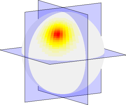
(b) Sphere with a bump

(c) Final computation

1. Introduction

Topological data analysis [3, 15] looks to quantify the qualitative aspects of the geometry of a data set. The existence and location of voids in an otherwise densely present figure are among the topological features we can try detect. The formalism of homology allows us to do this. It has had a large impact: both in geometry and mathematics in general, and more recently in a computational topology and geometry setting. The key to the success of homology in computational geometry, as well as in other application fields – is the introduction in [13] of persistent homology, a multi-scale approach to the computation of homological features given a point cloud of samples.

The original persistence algorithm [13] has a worst case, a $O(n^{3})$ running time . There has been considerable effort looking for more efficient algorithms for computing persistence. For special cases, such as 2-manifolds [13], very efficient, nearly linear algorithms exist. In the general case, recent progress has shown that persistence can be computed in matrix multiplication time [22] or alternatively in an output sensitive way [5]. These running times are given in terms of simplices, so another active line of research is into using discrete Morse-theoretic methods or homotopical collapses [20, 24, 23, 25, 17, 11] to reduce the size of the underlying complex while ensuring the resulting homology computation gives the correct result. These are particularly useful when the underlying complex is described by a simpler object such as its graph [29, 30, 9] (i.e. for flag complexes).

The standard algorithm is most often used, since in practice, it has almost linear runtime. The algorithm depends on having random access to a representation of the boundary operator. The standard representation is as a sparse matrix and during the course of the standard algorithm in higher dimensions, the matrix quickly fills-in requiring $O(n^{2})$ storage space. In practice, the requirement of random access to such a large data structure has proven to be the limiting factor in computation. There has been work on distributed computation, primarily focusing on ordinary homology in sensor networks and using either coreduction techniques as above [10] or via combinatorial Laplacians [26]. The latter approach does not readily extend to persistent homology and is much slower in practice than centralized methods.

In this paper, we present an algorithm which uses a divide-and-conquer approach to computing both homology and persistent homology. Rather than computing on the entire complex, we break the computation up into smaller pieces. The benefit being that we can compute persistence independently on the each of the pieces or patches. The key contirbution of this paper is to show how to merge the results from the individual patches into a global quantity. Our approach is based on a tool from algebraic topology called spectral sequences. Dividing the space up based on a cover $\mathcal{U}$, the spectral sequence gives the machinery necessary to iteratively compute better approximations of the persistent homology of a total space $\mathbb{X}$ from the local persistence computations in each $\mathbb{U}_{i}\in\mathcal{U}$.

We focus our attention on the underlying ideas based on spectral sequences and the resulting algorithms rather than on the analysis of these algorithms, which depend heavily on the cover (i.e. how we break up the underlying complex). We partially address the problem of computing covers by presenting some straightforward approaches which could be used. Using the developed techniques also gives a more convenient form of the Nerve [19] and Persistent Nerve [4] lemmas which are widely used in persistent homology, as well as an algebraic description of the image, kernel and cokernel persistence introduced in [7].

The paper is structured as follows: we first introduce the Mayer-Vietoris spectral sequence, which is the main algebraic tool that will be used in the paper. We adapt the treatement of [16] to a persistent homology context, and provide mathematical descriptions of the spectral sequence computation. Using these structural results, in Section 3 we give explicit descriptions of all the needed algorithms; from basic algebraic primitives computing kernels, images and cokernels of maps between finitely presented $\mathbb{k}[t]$-modules to the concrete computation of the spectral sequence. Finally, in Section 5 we discuss several applications and corollaries to the theory and algorithmics in this paper. In particular, we discuss strategies for parallelizing persistence and for computing persistent homology with a stratified memory residence approach; the relationship between our algebraic primitives and the corresponding geometric primitives in [7]; and we give proofs of the homological Nerve lemma and of the persistent homological Nerve lemma that avoid the requirement of contractibility of all the covering patches and patch intersections.

1.1. Background

For an introduction to persistent homology we refer the reader to [12, 28] along with [19] for an introduction to homology within algebraic topology. The main object which we look to compute is the persistence module. This is an algebraic object introduced in [31], which encodes the homology of a filtration, a sequence of increasing simplicial complexes

$$\emptyset=\mathbb{X}_{0}\subseteq\mathbb{X}_{1}\subseteq\ldots\subseteq\mathbb{X}_{n-1}\subseteq\mathbb{X}_{N}=\mathbb{X}$$

The module encodes the information in all pairwise maps between these spaces. It turns out that, this information can be represented by a barcode or persistence diagram which are a set of coordinates which represent the birth and death times of non-trivial homology classes in the filtration.

These have geometrical meaning if the filtration is derived from some geometric quantity. Common examples include: the sub-level set filtration with respect to some function defined on the space and the filtration based on distances between points in an input point cloud.

In this paper, we compute homology over coefficients in a field $\mathbb{k}$. In this case, the homology over a space is a vector space. However, as shown in [31], rather than computing the homology for each space independently, we can build graded $\mathbb{k}[t]$-linear chain complexes where the degree of each generator encodes the entry of a simplex into the filtration. Refering to this as persistence complex, the authors show that persistent homology is equivalent to ordinary homology on the persistence complex with coefficients in $\mathbb{k}[t]$.

The division of our space will be in terms of a cover. A cover of a space $\mathbb{X}$ is an indexed family of sets $\mathbb{U}_{i}$ such that $\mathbb{X}\subseteq\cup_{i}\mathbb{U}_{i}$. The methods we develop work with arbitrary covers of the space, making the method suitable for any division of the underlying space (of course, the performance will depend on the properties of the cover). Much of the exposition is given in the language of commutative algebra. This not only simplifies the exposition, but gives important insight into how the algorithms should work. Whereever possible, we try to put things into the context of previous approaches.

2. The Mayer-Vietoris spectral sequence

Spectral sequences have seen numerous uses in classical algebraic topology [21]. In the field of persistent homology, an awareness of the role of spectral sequences has been present from the start [31], but the difficulty in computing with spectral sequences has consistently made alternative routes attractive. We do not give a complete background on spectral sequences here but rather, we focus our attention on one particular spectral sequence, which we use for the parallelization of persistent homology. For reference, spectral sequences are discussed extensively in [21] although more accessible introductions can be found in [6] and [18].

The spectral sequence we use can be viewed as generalization of the Mayer-Vietoris long exact sequence which given two pieces, relates the homology of their union with the homology of the pieces and their intersection. The same way that the long exact sequence encodes an inclusion-exclusion principle on homology classes, the corresponding spectral sequence provides the mechanics of an inclusion-exclusion principle for deeper intersections than the pairwise afforded by the long exact sequence. Frequently mentioned in the literature (inter alia: [21]), we found the most detailed expositions in [1, 2, 16]. The spectral sequence builds up a space very similar to the blowup complex introduced by Carlsson and Zomorodian in [32], but uses more of the available information in order to knit together local information to a global homology computation. Also Carlsson and Zomorodian do not use the same filtration as we depend on here. The following is based very loosely on the exposition in [16].

As in [32], we consider a filtered simplicial complex $\mathbb{X}$, with a cover $\mathcal{U}$ by filtered subcomplexes $\mathbb{X}=\bigcup_{i\in\mathbb{I}}\mathbb{U}_{i}$ (see Figure 1(b)). The cover can of course be anything, but in practice we wish to divide the full filtered complex into almost disjoint pieces so as to maximally parallelize the computation. The condition of covering with filtered subcomplexes is trivially fulfilled if we construct the cover on the final space of the filtration.

We recall the definition of the blowup complex from [32]

$$\mathbb{X}^{\mathcal{U}}=\bigcup_{\emptyset\neq J\subseteq\mathbb{I}}\left(\bigcap_{j\in J}\mathbb{U}_{j}\right)\times\Delta^{J}$$

where $\Delta^{J}$ is the $|J|$-simplex with vertices numbered from $J$.

Fundamentally, the question is how we can compute the homology of the blowup complex. We approach this by separating out the problem into computational components. Whenever $n$, $p$ and $q$ occur simultaneously, we shall assume that $n=p+q$. The $q$-chains in a $p$-fold intersection of the original cover generate $p+q$-chains in the chain complex of the blowup complex, and thus potentially $p+q$-homology.

(d) An underlying topological space covered by three sets.

(e) The sets shown as disjoint spaces.

(f) Blowup complex.

Figure 1. Construction of the blowup for a triple cover. In the blowup (c), anything in a double intersection is multiplied with an edge, and anything in a triple intersection is multiplied by a 2-simplex. While only visible in the top right one, all three parts of the curve going through a double intersection will be replaced by a triangulated quadrilateral.

We use this to organize our computation. Let us write $E^{0}_{p,q}$ for the $q$-chains in a $p$-fold intersection of the original cover. The individual chain complexes $E^{0}_{p,*}$ have boundary maps inherent from their simplicial complex structure, and we shall write $d^{0}_{p,q}$ for the map $E^{0}_{p,q}\to E^{0}_{p,q-1}$, and $d^{0}$ for the aggregate map $E^{0}_{*,*}\to E^{0}_{*,*}$.

(a) Double complex expression of the $E^{0}$ page.

(b) Typical element of the total complex.

Figure 2. Double complex setup. A double complex is a grid as depicted in (a), with modules at each grid point, and two families of maps $d^{0}$ and $d^{1}$ between the modules. For a double complex, we require $d^{0}d^{1}+d^{1}d^{0}=0$ as well as $d^{0}d^{0}=0$ and $d^{1}d^{1}=0$. A typical element of the total complex is some tuple $(\alpha_{0},\dots,\alpha_{n})$, and will map under the total differential to some other element $(\omega_{0},\dots,\omega_{n-1})$ given by summing up the contributions from each direction.

For any particular $J\subseteq\mathbb{I}$, and any particular $j^{\prime}\in J$, there is an inclusion map $\bigcap_{j\in J}\mathbb{U}_{j}\to\bigcap_{j\in J\setminus j^{\prime}}\mathbb{U}_{j}$. If we multiply each such inclusion map with the sign of the corresponding term $J\to J\setminus j^{\prime}$ of the nerve complex boundary map, and sum the maps up for all $j^{\prime}$, we get a map $d^{1}_{p,q}:E^{0}_{p,q}\to E^{0}_{p-1,q}$. Aggregating over all chains, we have a map $d^{1}:E^{0}_{*,*}\to E^{0}_{*,*}$.

A structure like this, with bi-indexed modules $E^{0}_{p,q}$ and horizontal maps $d^{0}$ and vertical maps $d^{1}$ such that $d^{0}\circ d^{0}=0$, $d^{1}\circ d^{1}=0$ and $d^{0}\circ d^{1}+d^{1}\circ d^{0}=0$ is called a double complex. For double complexes, we can generate a straightforward chain complex called the total complex by writing $\mathop{\mathrm{Tot}}(E^{0}_{*,*})_{n}=\bigoplus_{p+q=n}E^{0}_{p,q}$, and introduce as a boundary map the aggregate map $d^{0}+d^{1}$.

For our computation of the homology of the blowup complex, we rely on a fundamental theorem from algebraic topology [16]:

Theorem 1.

$H_{*}(\mathop{\mathrm{Tot}}(E^{0}_{*,*}))=H_{*}(\mathbb{X})$.

While we shall not prove the theorem in its full extent here, we still need the statement of the isomorphism for the development of our algorithm. A chain in $E^{0}_{1,q}$ is a collection of $q$-chains in the covering patches. Such a chain can be mapped into $C_{*}\mathbb{X}$ by simply summing up the component chains, included into the full complex. Just summing up these components may both introduce and remove homological features present in the composite chain – and the exact behaviour of these introductions and removals is encoded into the other summands of the direct sum. Thus, the isomorphism identifies a class $[(\alpha_{0},\dots,\alpha_{n})]$ with a class $[\alpha]$ precisely if $\alpha$ is the result of summing up the components of $\alpha_{0}$. The chains $\alpha_{1},\dots,\alpha_{n}$ capture, in a way reminiscent of the inclusion-exclusion principle, the exact ways in which $\alpha$ differs from merely summing up $\alpha_{0}$.

The columns in the double complex provide a filtration on $\mathop{\mathrm{Tot}}(E^{0}_{p,q})$. We write $E^{0}_{\leq p,*}$ for the subcomplex consisting of the $p$ leftmost columns, and write $L_{n,p}=\mathop{\mathrm{im}}(H_{n}(\mathop{\mathrm{Tot}}(E^{0}_{\leq p,*}))\to H_{n}(\mathop{\mathrm{Tot}}(E^{0}_{*,*})))$ for the image of the map induced by the inclusion of a particular filtration step into the entire double complex. Since the $E^{0}_{\leq p,*}$ filter $E^{0}_{*,*}$, the $L_{n,p}$ filter $H_{n}(\mathop{\mathrm{Tot}}(E^{0}_{*,*}))$. Furthermore, a single class $[(\alpha_{0},\dots,\alpha_{n})]$ is in $L_{n,p}$ if and only if the class has a representative on the form $(\alpha^{\prime}_{0},\dots,\alpha^{\prime}_{p},0,\dots,0)$.

While computing $L_{n,p}$ completely ends up being similar in difficulty to the original homology computation, we can consider the computation of just the elements that get added at any particular step of the filtration. In other words, if we compute $L_{n,p}/L_{n,p-1}$, this tells us about only those elements of $H_{*}(\mathbb{X})$ that show up at precisely the $p$-fold intersections. Clearly, taking the direct sum over all $p$ of these quotients, we can compute a complete description of the entire homology $H_{*}(\mathbb{X})$.

Given some element $[(\alpha_{0},\dots,\alpha_{p},0,\dots,0)]\in L_{n,p}$, the equivalence class it belongs to in $L_{n,p}/L_{n,p-1}$ is completely determined by the value of $\alpha_{p}$. The particular $\alpha_{p}$ representing such an element is not uniquely determined, nor is every element of $E^{0}_{p,q}$ a valid choice for some element determining an equivalence class of $L_{n,p}/L_{n,p-1}$. We shall write $Z^{\infty}_{p,q}$ for the $\alpha_{p}$ that do represent some equivalence class of $L_{n,p}/L_{n,p-1}$, and we shall write $B^{\infty}_{p,q}$ for the elements of $E^{0}_{p,q}$ that represent the 0 class of $L_{n,p}/L_{n,p-1}$.

The spectral sequence here aims to provide increasingly accurate approximations to these $Z^{\infty}_{p,q}$ and $B^{\infty}_{p,q}$. These approximations are computed by introducing the conditions defining $Z^{\infty}_{p,q}$ and $B^{\infty}_{p,q}$ one at a time.

The case $Z^{r}_{p,q}$

Fix some $\alpha_{p}\in E^{0}_{p,q}$. For $\alpha_{p}$ to be in $Z^{\infty}_{p,q}$, there has to be a sequence $\alpha_{p-1},\dots,\alpha_{0}$ as in Figure 3 (a) such that

(1) $$d^{0}\alpha_{p}=0\qquad d^{0}\alpha_{p-1}=d^{1}\alpha_{p}\qquad\dots\qquad d^{0}\alpha_{0}=d^{1}\alpha_{1}$$

These equations express the condition $d(\alpha_{0},\dots,\alpha_{p},0,\dots,0)=0$ in $\mathop{\mathrm{Tot}}(E^{0}_{*.*})$.

We define $Z^{r}_{p,q}$ to be the set of all $\alpha_{p}$ that fulfill the conditions

(2) $$d^{0}\alpha_{p}=0\qquad d^{0}\alpha_{p-1}=d^{1}\alpha_{p}\qquad\dots\qquad d^{0}\alpha_{p-r}=d^{1}\alpha_{p-r+1}$$

and in particular, we can compute $Z^{r}_{p,q}$ recursively as those elements $\alpha_{p}$ of $Z^{r-1}_{p,q}$ for which there in addition to the $\alpha_{p-1},\dots,\alpha_{p-r+1}$ elements guaranteed to exist since $\alpha_{p}\in Z^{r-1}_{p,q}$, there is also an $\alpha_{p-r}\in E^{0}_{p-r,q+r}$ such that $d^{0}\alpha_{p-r}=d^{1}\alpha_{p-r+1}$. It is clear from these definitions that $Z^{p}_{p,q}=Z^{\infty}_{p,q}$.

The case $B^{r}_{p,q}$

As above, we fix $\alpha_{p}\in E^{0}_{p,q}$. In order for $\alpha_{p}$ to be in $B^{\infty}_{p,q}\subseteq Z^{\infty}_{p,q}$, we additionally need a collection of elements $\beta_{p},\dots,\beta_{n+1}$ as in Figure 3 (b) such that

(3) $$d^{0}\beta_{p}+d^{1}\beta_{p+1}=\alpha_{p}\qquad d^{0}\beta_{p+1}+d^{1}\beta_{p+2}=0\qquad\dots\qquad d^{0}\beta_{n}+d^{1}\beta_{n+1}=0$$

The simplest case when this happens is if there is some $\beta_{p}$ such that $d^{0}\beta_{p}=\alpha_{p}$. In this case we can choose $\beta_{j}=0$ for all other $\beta_{j}$. We write $B^{0}_{p,q}$ for the vector space of all such $\alpha_{p}$.

In general, we shall define $B^{r}_{p,q}$ to be the set of $\alpha_{p}$ for which there are $\beta_{p},\dots,\beta_{p+r}$ satisfying the equations

$$d^{0}\beta_{p}+d^{1}\beta_{p+1}=\alpha_{p}\qquad d^{0}\beta_{p+1}+d^{1}\beta_{p+2}=0\qquad\dots\qquad d^{0}\beta_{p+r-1}+d^{1}\beta_{p+r}=0\qquad d^{0}\beta_{p+r}=0$$

In particular $\alpha_{p}\in B^{r}_{p,q}$ if $\alpha_{p}\in B^{r-1}_{p,q}$ or if there are $\beta_{p},\dots,\beta_{p+r}$ satsifying all these equations.

(a) Condition for a cycle: $(\alpha_{0},\dots,\alpha_{2},0,\dots,0)$ is a cycle if there are $\omega_{0},\omega_{1}$ such that $d^{0}\alpha_{0}=\omega_{0}=d^{1}\alpha_{1}$, $d^{0}\alpha_{1}=\omega_{1}=d^{1}\alpha_{2}$ and $d^{0}\alpha_{2}=0$.

(b) Condition for a boundary: $(\alpha_{0},\dots,\alpha_{2},0,\dots,0)$ is a boundary if in addition to the $\omega_{0},\omega_{1}$ in (a), there are also $\beta_{2},\dots,\beta_{5}$ such that $d^{0}\beta_{2}+d^{1}\beta_{3}=\alpha_{2}$, $d^{0}\beta_{3}+d^{1}\beta_{4}=0$, $d^{0}\beta_{4}+d^{1}\beta_{5}=0$ and (trivially) $d^{0}\beta_{5}=0$.

Figure 3. Cycles and boundaries in $E^{r}_{p,q}$.

$Z^{r}_{p,q}$ and $B^{r}_{p,q}$ as kernel and image of a differential

Suppose $\alpha_{p}\in Z^{r}_{p,q}$. Then there exist $\alpha_{p-1},\dots,\alpha_{p-r}$ as above. Let $\omega_{p-r-1}=d^{1}\alpha_{p-r}\in Z^{r}_{p-r-1,q+r}$. This element is well-defined, depending only on $\alpha_{p}$, up to a sequence of error terms for all the $\alpha_{p-i}$, each of which is guaranteed to be in the appropriate $B^{r}_{p-i,q+i}$. Hence, the map $[\alpha_{p}]\mapsto[\omega_{p-r-1}]$ is a well-defined map $d^{r}:Z^{r}_{p,q}/B^{r}_{p,q}\to Z^{r}_{p-r-1,q+r}/B^{r}_{p-r-1,q+r}$. This collection of quotient modules is often denoted $E^{r}_{p,q}=Z^{r}_{p,q}/B^{r}_{p,q}$ and called the $E^{r}$-page.

The elements $\alpha_{p},\dots,\alpha_{p-r}$ are an appropriate set of $\beta_{j}$ to witness $\omega_{p-r-1}\in B^{r}_{p-r-1,q+r}$. Re-indexing, we can conclude that $\alpha_{p}\in B^{r+1}_{p,q}$ if and only if $[\alpha_{p}]=d^{r}[\beta_{p+r+1}]$ for some $\beta_{p+r+1}\in Z^{r}_{p+r+1,q-r}$.

Finally, if $w_{p-r-1}\in B^{r}_{p-r-1,q-r}$, or equivalently if $d^{r}[\alpha_{p}]=[0]$, then it follows that $\alpha_{p}\in Z^{r}_{p,q}$.

All these statements can be easily proven by diagram chases.

If at any stage of the computation, all the maps $d^{r}:E^{r}_{*,*}\to E^{r}_{*,*}$ are the zero-map, then the corresponding $Z^{r}_{*,*}$ and $B^{r}_{*,*}$ already satisfy all their conditions, and so for that $r$, it already holds that $Z^{r}_{*,*}=Z^{\infty}_{*,*}$ and $B^{r}_{*,*}=B^{\infty}_{*,*}$. Many proofs in algebraic topology work by proving that for a low value of $r$, the map $d^{r}$ vanishes, eliminating the need to construct the higher index maps. In Section 5.3 we shall see an application of this principle.

3. Algorithms

We shall state algorithms here both for the underlying algebraic operations, as well as for the resulting spectral sequence and persistence computations.

3.1. Algebraic operations

In algebra textbooks written with a sufficiently general approach to linear algebra, the development of matrix arithmetic and its uses in solving linear equations will be done in a manner appropriate for a generic Euclidean domain [27]. It is a well-known fact that in addition to any field, further Euclidean domains include $\mathbb{Z}$, as well as $\mathbb{k}[t]$ for any field $\mathbb{k}$. In this setting, a few useful facts hold: any submodule of a free module is free, and Gaussian elimination is an appropriate algorithm to compute matrix ranks, function kernels and images, reducing bases to remove redundancies and to form appropriate reduction systems.

In light of this, we draw the reader’s attention to the implications for persistence. A persistence chain complex is a free graded $\mathbb{k}[t]$-module with a generator in degree $k$ for each simplex that enters the filtered chain complex in the $k$th filtration step. Persistent homology is a finitely presented graded $\mathbb{k}[t]$-module, with generators given by a cycle basis and relations given by a boundary sub-basis of the cycle basis.

We can assume – especially in the topological case – that if some $t^{k}\sum\lambda_{j}t^{j}m_{j}$ is a boundary basis element, then the cycle was a cycle already $k$ time-steps earlier, represented by $\sum\lambda_{j}t^{j}m_{j}$. We shall represent finitely presented modules precisely as a segregated pair of bases: a generators basis and a separate relations basis. Because of this nice behaviour of the generators corresponding to specific relations, we can further allow ourselves to keep the relations basis in a row-reduced form – to ensure that the division algorithm produces nice normal forms of all elements – and the generators basis reduced with respect to the relations.

As the reader recalls, Gaussian elimination puts a matrix into a normal form by clearing out row by row by using the leftmost column in the matrix with no non-zero entries above of the current row to cancel out any entries occurring later. When working with graded $\mathbb{k}[t]$-modules, some care has to be taken to avoid reducing any columns using columns that do not exist in an early enough grading. This can be accomplished by sorting the columns in the matrix in order of rising degree, and only reducing to the right. Tracking the operations performed during a reduction allows for the computation of a kernel by reading off the operations that produced all-zero columns in the reduced matrix.

Given a function $f:M/Q\to N/P$, where $M/Q$ and $N/P$ are both represented by lists of generators and lists of relations as discussed above, the following three constructions come naturally:

Image modules

To compute $\mathop{\mathrm{im}}f$, we compute the list $f(m)$ for $m\in M$. Since $f(Q)\subseteq P$, the relations on $\mathop{\mathrm{im}}f$ are the relations listed in $P$, and so $\mathop{\mathrm{im}}f=f(M)/P$.

Cokernel modules

To compute $\mathop{\mathrm{coker}}f$, we need to compute $(N/P)/(f(M/Q))$. Again, $f(Q)\subseteq P$, and thus we get the resulting module by imposing all the images $f(m)$ of the generators of $M$ as additional relations. Hence, $\mathop{\mathrm{coker}}f=N/(f(M)\cup Q)$.

Kernel modules

The kernel is, just as in [7], more complex than the image and cokernel. The computation of the kernel module as well as its embedding into $M/Q$ is computed in a two-step process. An element of $\ker f$ is going to be represented by some element of the free module $M$ such that $f(m)\in P$. We can compute this by computing the kernel $F_{K}$ of the map $M\oplus P\to N$ given by $(m,p)\mapsto f(m)-p$. This is a kernel of a map between free $\mathbb{k}[t]$-modules, and thus computable with the matrix algorithm above. The actual generators in $M$ are given by the projection onto the first summand $\pi_{M}:(m,q)\mapsto m$, and we write $K=\pi_{M}(F_{K})$.

The resulting elements form a free submodule of $M$ giving generators of the kernel module. The kernel module will have relations, however, and not all relations in $Q$ are going to be in the submodule $K$. Hence, for a full presentation, we need to find the relations that are actually in $K$, which we can do with another kernel computation. We consider the map $K\oplus Q\to M$ given by $(k,q)\mapsto k-q$ and compute its kernel. The projection $\pi_{K}:(k,q)\mapsto k$ gives us a set of relations.

The constructions above, as well as Gröbner basis approaches to handling free modules over polynomial rings are described in [14].

3.2. Spectral sequence differentials

Using the algebraic operations described above, we describe an algorithm for computing persistent homology via the Mayer-Vietoris spectral sequence. This algorithm is iterative and converges to the correct cycles $Z^{\infty}$ and boundaries $B^{\infty}$ so that the isomorphism in Theorem 1 holds.

Converge occurs when the spectral sequence collapses. In particular, if the differential $d^{r}$ is the zero-map everywhere, then $Z^{r+1}=Z^{r}$, and $B^{r+1}=B^{r}$, and we can verify that $d^{r+1}$ is also going to be the zero-map everywhere, and this continues all the way up. One powerful use of this is that once the maps $d^{r}$ traverse the double complex in such a way that they only hit trivial modules, the corresponding $d^{r}$ has to be the zero-map. This happens, for instance, if the double complex is contained in a $p\times q$ bounding box where $p$ and $q$ are maximal dimensions of the complex and nerve respectively. In this case, the spectral sequence will collapse for $r>\min(p,q)$. At that point all the maps will map outside the box and so can only hit trivial modules.

We first describe the initialization of the algorithm. Beginning with the double complex of Figure 2(a), we first compute homology vertically, replacing each $E^{0}_{p,q}$ with the quotient module $Z^{1}_{p,q}/B^{1}_{p,q}$ where $Z^{1}_{p,q}=\ker d^{0}_{p,q}$ and $B^{1}_{p,q}=\mathop{\mathrm{im}}d^{0}_{p,q+1}$. This computes, in effect, the persistent homology of the chain complex over each simplex in the nerve of the cover. We represent $E^{1}_{p,q}$ by its segregated basis, as described in Section 3.1, maintaining the free modules $Z^{1}_{p,q}$ and $B^{1}_{p,q}$ as well as the preboundary $I^{1}_{p,q}$ defined by the equation $d^{0}_{p,q}I^{1}_{p,q}=B^{0}_{p,q-1}$.

Next, we describe the iterative step. We will, for now, assume that we are given the differentials and describe their computation afterwards.

At the $r$-th iteration, at each node $(p,q)$, we compute the kernel module of $d^{r}_{p,q}$, storing it as $Z^{r}_{p,q}$ and the image module of $d^{r}_{p+r-1,q-r}$, storing this as $B^{r}_{p,q}$. Since $d^{r}$ is a differential, we know that $B^{r+1}_{p,q}\subseteq Z^{r+1}_{p,q}$, and by reducing both generating sets we can find a good presentation of the quotient $Z^{r+1}_{p,q}/B^{r+1}_{p,q}=E^{r+1}_{p,q}$.

As for the concrete maps $d^{r}$, we compute them as we go along. In particular, $d^{1}$ is the induced map on $E^{1}$ by giving the inclusion maps of deeper intersections into more shallow the coefficients from the nerve boundary map. The higher differentials $d^{r}$ are computed according to the machinery of Section 2. In particular, the images of $d^{r-1}_{p,q}$ are retained. For an element $x\in E^{r}_{p,q}$ in the kernel of $d^{r-1}_{p,q}$ we can find a corresponding image element $d^{r-1}_{p,q}x\in B^{0}_{p-r+2,q+r-1}$. Therefore, we can find some $y\in I^{1}_{p-r+2,q+r}$ such that $d^{0}_{p-r+2,q+r}y=d^{r-1}_{p,q}x$. We define $d^{r}x=d^{1}y$. This corresponds precisely to the description in Section 2, where the theoretical motivation can be found explaining exactly why these operations are all possible to perform and appropriate. In each iteration, we use the image and kernel module computations between finitely presented modules and maps that are computed in earlier stages.

For a lower level description of the algorithm see Appendix B.

4. Explicit example

Consider the sphere in Figure 4(a). Its function will introduce the hot spot and its surrounding area significantly later than the remaining sphere. Computing persistence over the entire sphere, we would expect to see a signature somewhat like the one in Figure 4(c).

(a)

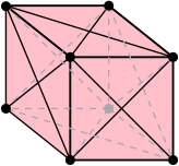
(b)

(c)

Figure 4. (a) A sphere with constant function everywhere except one hotspot. The partition of the space is along the axes. Each partition is then thickened slighlty as described in Section 5.1 to give the covering. (b) The nerve of the covering. Note that the faces have tetrahedra as all 4 vertices of the square intersect. (c) The persistent barcode of the sphere, $H_{1}$ is trivial so it is not shown.

We can divide the computation on the sphere into octants divided by the axis planes, as in Figure 4(a) and (b). By growing each octant by the tubular neighbourhood method in Section 5.1, we get separate computational units, with contractible intersections of all higher orders. Hence, after computing persistent homology on all patches, and on pairwise, triple and quadruple intersections, we get a double complex of persistence modules shown in Figure 5(b).

(a) $E^{1}$ page.

(b) Computing $d^{2}$ on $E^{2}$.

(c) $E^{3}$ page, collapsed spectral sequence.

Figure 5. Example computation for the sphere.

The exponents come from the 6 vertices of the octahedron generating 6 quadruple intersection. In each of these, there are 4 different triple intersections, generating a total of 24 triple intersections. Each of the 6 tetrahedra has 6 edges, corresponding to all the double intersections at each vertex – however, this overcounts each the 12 double intersections corresponding to edges of the octahedron. Thus, out of the 36 double intersections, only 24 remain after compensating for the overcounting. Finally, each of the 8 faces of the octahedron corresponds to a single covering patch.

After computing the corresponding $E^{2}$-page, the redundancies in the duplicate representations of all components have largely resolved, and we are left with a double complex of persistence modules shown in Figure 5(b). Here, the map $k[t]\to k[t]/t^{m}$ maps the generator onto the generator. The kernel of this map is $t^{m}k[t]\subset k[t]$, and the image is the entire module. This gives our final page of the spectral sequence shown in Figure 5(c). Reading off the modules diagonally, we recover the persistent homology groups $H_{0}=k[t]$ and $H_{2}=t^{m}k[t]$, which is precisely what we computed before.

5. Applications

5.1. Computing partitions

The input to use the Mayer-Vietoris spectral sequence is a filtered simplicial complex is covered by subcomplexes. Given a point cloud $\mathbb{X}$, and a method $C_{*}$ (such as Vietoris-Rips or Witness complexes) to construct filtered a simplicial complex $C_{*}\mathbb{X}$ from $\mathbb{X}$, we shall describe a few schemes to divide $C_{*}\mathbb{X}$ into a covering by appropriate subcomplexes with small intersections. Minimizing the size of the intersections, we minimize the amount of work which must be done in higher pages.

Recall that the closed star in a simplicial complex of a subset of its simplices is the subcomplex consisting of all simplices that intersect any simplex in the subset. We now state two lemmas and refer the reader to Appendix A for the proofs.

Lemma 2.

Suppose $C_{*}$ has the property that any simplex has diameter at most $\varepsilon/2$, and that the presence of any simplex is decided using points of a distance at most $\varepsilon/2$ from any of the vertices of the simplex.

Then the closed star of a subset $S\in C_{*}\mathbb{X}$ is going to be contained in $C_{*}T_{\varepsilon}S$ for $T_{\varepsilon}S$ the $\varepsilon$-tubular neighbourhood of $S$ in $\mathbb{X}$, the collection of points $x\in\mathbb{X}$ such that $d(x,S)<\varepsilon$.

Lemma 3.

Suppose $\mathbb{X}$ is partitioned into subsets $\mathbb{U}_{j}$. Then a covering of $C_{*}\mathbb{X}$ by subcomplexes is given by the collection of subcomplexes $C_{*}T_{\varepsilon}\mathbb{U}_{j}$.

We now describe some concrete methods for computing the covers.

Cube partitions

Suppose $\mathbb{X}$ is a subset of some Euclidean space $\mathbb{R}^{n}$. Cover $\mathbb{X}$ by a disjoint collection of axis-parallel cubes. Membership in a particular cell is quickly computed by comparing the coordinates of the points in $\mathbb{X}$ to boundaries for the cubes. A covering of $C_{*}\mathbb{X}$ is given by the closed stars of the cells, easily computable as $C_{*}T_{\varepsilon}\mathbb{U}_{j}$ for points in the tubular neighborhoods of the cells.

Voronoi partitions

Pick some collection of landmark points $L\subset\mathbb{X}$. Compute Voronoi regions $V_{\ell}$ for $\ell\in L$. As above, we construct a covering of $C_{*}\mathbb{X}$ by closed stars of the Voronoi cells, computable as $C_{*}T_{\varepsilon}\mathbb{U}_{j}$.

Geodesic Voronoi partitions

Pick some collection of landmark points $L\subset\mathbb{X}$. Let $C_{*}$ be a method that constructs a flag complex on some graph induced by the geometry of $\mathbb{X}$. Write $d_{\Gamma}$ for the geodesic graph distance, given by $d_{\Gamma}(x,y)$ equal to the least number of edges from $x$ to $y$ in $\Gamma$. Write $\mathbb{U}_{\ell}$ for the set $\{y\in\mathbb{X}:d_{\Gamma}(x,\ell)<d_{\Gamma}(x,\ell^{\prime})\forall\ell^{\prime}\in L\setminus\ell\}$, or in other words the set of points closer to $\ell$ than to any other point in $L$.

As a covering by subcomplexes, we grow each $\mathbb{U}_{\ell}$ to $\mathbb{U}^{\prime}_{\ell}$ by including all immediate neighbours of the points in $\mathbb{U}_{\ell}$. A covering of $\mathbb{X}$ by subcomplexes is given by the flag complexes on $\mathbb{U}^{\prime}_{\ell}$.

(a)

(b)

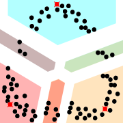
(c)

(d)

Figure 6. Regions for Vietoris-Rips in an ambient Voronoi decomposition. From a pointcloud (far left) we pick three landmark points, and get a Voronoi decomposition of the ambient space (middle left). By growing each Voronoi region by $\varepsilon$, we get a covering of the point cloud satisfying the conclusion in Lemma 3 (middle right). The $\varepsilon$-Vietoris-Rips complexes in each of the covering patches and their intersections (far right) will provide a covering of the $\varepsilon$-Vietoris-Rips complex of the entire point cloud by subcomplexes.

5.2. Parallelism and stratified memory

Parallelisation with a covering is performed by splitting responsibility for the chain complex of a single covering patch or patch intersection to a single computational task. These tasks communicate with each other to update the global state in the horizontal differential parts of the computation, and perform boundary map preimage computations internally. If a computational node is responsible for chains over a single simplex of the nerve complex, it will only communicate with nodes representing simplices in its closure and its star. This can be seen since in the first iteration, that node will only need to communicate with the nodes responsible for its faces and cofaces. In the second iteration, it must communicate with the faces of its faces and cofaces of its cofaces.

To compute the total number of communications produced, we only consider communication at the level of the nerve of the covering rather than the size of the underlying simplicial complex. To avoid double counting, we only consider communication from a simplex into its closure.

To get a worst-case bound, we assume that the number of iterations required is equal to the maximal dimension of the nerve which we denote with $r$. Over all iterations, a $d$-simplex may produce no more than $O(2^{d})$ communications. This follows from the assumption that $r>d$ and the fact that the size of a $d$-simplex’s closure is $2^{d}$. If we denote the number of $i$-dimensional simplices in the nerve with $K_{i}$ and assume $r$ is the maximal dimension of the nerve, the total number of communications is $\sum_{i=1}^{r}K_{i}2^{i}$. This is very rough and pessimistic bound. We intend to do a more detailed analysis in future work.

We note that this approach will also be applicable in a single-processor context. Instead of distributing computational tasks on separate nodes, we can consider each subcomplex or subcomplex intersection a memory block. This way, the spectral sequence approach structures a computation, grouping accesses to related memory blocks into cohesive computational tasks, which induces swap schemes and schemes for stratified memory access.

5.3. Nerve lemma

The Nerve lemma [19, Corollary 4G.3] is a powerful result from algebraic topology that has seen repeated use in computational topology – all the way from motivating why the commonly used filtered simplicial complex constructions capture the original topology [3] to generating particular new results.

Quite often, when computational topologists use the Nerve lemma, quite a lot of effort is expended to provide the contractibility conditions required in the classical statement of the Nerve lemma. This is due to the most common form of the Nerve lemma guarantees both homological and homotopical equivalence between a covering and its nerve. As we are usually only interested in homology, we observe that the Mayer-Vietoris spectral sequence yields a proof of a homological Nerve lemma:

Theorem 4 (Homology Nerve lemma).

Suppose a space $\mathbb{X}$ is covered by a collection $\mathcal{U}$ of subspaces $\mathbb{X}=\bigcup_{i}\mathbb{U}_{i}$, such that each $\bigcap_{j}\mathbb{U}_{j}$ has trivial reduced homology in all degrees. Then $H_{*}(\mathbb{X})=H_{*}(\mathcal{N}(\mathcal{U}))$.

Proof.

On the $E^{1}$-page, the non-reduced homology is concentrated in degree 0. Since by assumption, the reduced homology is trivial for each intersection, the non-reduced homology is just a copy of the ground field. The differential on the $E^{1}$-page is the differential of the nerve complex itself, and the result follows immediately. ∎

While this is a well-known fact in classical algebraic topology, we point this out to emphasize that the intersections need not be equipped with explicit contracting homotopies for the Nerve Lemma to work in homological computations.

Persistent Nerve Lemma:

The Nerve Lemma was extended to the persistence setting in [4] using similiar homotopical arguments. Here, we give the spectral sequence version of it which relies on a persistent acyclicity condition.

From our framework also follows a persistent Nerve lemma.

Definition 5.

A space is persistently acyclic if it has persistent homology consisting of one free generator of $H_{0}$, and no homology in higher degrees.

Theorem 6 (Persistent homology Nerve lemma).

Suppose a filtered space $\mathbb{X}$ is covered by a collection $\mathcal{U}$ of filtered subspaces $\mathbb{X}=\bigcup_{i}\mathbb{U}_{i}$, such that each $\bigcap_{j}\mathbb{U}_{j}$ is persistently acyclic. Then $H_{*}(\mathbb{X})=H_{*}(\mathcal{N}(\mathcal{U}))$.

Proof.

We note that persistent homology is homology with coefficients in $\mathbb{k}[t]$. The persistent acyclicity condition ensures that homology has just one generator with the appropriate grading concentrated in the 0-homology. As in Theorem 4, the sequence collapses after the $E^{1}$ page and the $d^{1}$ differential is equivalent to the boundary operator of the nerve. The result follows. ∎

5.4. Algebraic kernel, cokernel and image persistence

In [7], the authors construct topological spaces that compute image, kernel and cokernel persistence modules for the map induced in persistent homology by a map between filtered topological spaces. We observe that the constructions in section 3.1 provide corresponding operations on a purely algebraic level, computing persistence modules for image, kernel and cokernel given a map of persistence modules, such as the one induced from a topological map.

The notion of compatible filtration included as a condition in [7] is reflected in the requirement that maps between persistence modules be graded module homomorphisms of degree 0, implying that the filtration inclusions on both sides commute with the map itself.

6. Discussion

We have constructed algorithms to compute with the spectral sequence generated by a double complex. In particular, we describe how to compute a spectral sequence generalizing the Mayer-Vietoris long exact sequence to compute both classical and persistent homology using a cover of the space and restricting computation to each of the covered regions and their intersections.

This layout enables us to formulate parallelization schemes, with parallelism and independency guarantees present both along the Nerve complex axis of our computational scheme and along separate components of the covering.

As an added bonus, the formalism of the spectral sequence approach suggests simplified proofs for several classical interesting results in the persistence community, and opens up a wide spectrum of interesting areas of research. In particular, we are interested in pursuing:

Complexity bounds for parallelism:

This paper presents the formalism, but does not attempt a complete description of the complexity behaviour of the proposed algorithms.

HPC implementation:

While the work was driven by a wish to take persistent homology to the world of computing clusters, our implementation so far is a serial one. A parallel implementation, and actual performance measurements would be very interesting.

Cover generation schemes:

While we give a few suggestions here, the construction of an adequate cover that uses or highlights inherent features of the dataset under analysis is going to be an important factor of these methods. A more complete catalogue of cover generation schemes is going to be important for the practical application of our techniques.

Theoretical implications:

We have already seen that several results have algebraic proofs that vastly simplify the arguments involved. We would be very interested in exploring the space of new or classical results that become accessible with a spectral sequence language.

Appendix A Proofs of selected results

Proof of Lemma 2.

Suppose $C_{*}$ determines the presence of a simplex using points at most $\varepsilon/2$ away from any point in a simplex, and each simplex has diameter at most $\varepsilon/2$. A simplex $\sigma$ in $C_{*}\mathbb{X}$ is in the closed star of $S$ if at least one vertex of $\sigma$ is in $S$. By the condition on the diameter, all other points of $\sigma$ are contained in $T_{\varepsilon/2}S$. In addition, any point that can influence the decision on whether $\sigma$ exists or not will be within $\varepsilon/2$ of the furthest point from the vertex of $\sigma$ in $S$, and thus the simplex $\sigma$ is entirely determined by points at most $\varepsilon$ away from $S$, and thus by $T_{\varepsilon}S$. ∎

Proof of Lemma 3.

If $\mathbb{X}$ is partitioned into subsets $\mathbb{U}_{j}$, we may certainly partition $C_{*}\mathbb{X}$ by the closed stars of the subsets. Indeed, since the $\mathbb{U}_{j}$ partition $\mathbb{X}$, we are guaranteed that any vertex of a simplex lies in at least one of the $\mathbb{U}_{j}$. Hence, in particular, the closed stars of all the $\mathbb{U}_{j}$ will contain all simplices in $C_{*}\mathbb{X}$.

By Lemma 2, each such closed star is contained in $C_{*}T_{\varepsilon}\mathbb{U}_{j}$. Hence, the subcomplexes $C_{*}T_{\varepsilon}\mathbb{U}_{j}$ cover $\mathbb{X}$. ∎

Appendix B Implementation

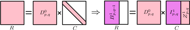
Figure 7. The basic reduction: As in [8], we reduce the matrix $R$ left to right, always choosing the lowest possible pivot with shaded areas representing non-zero entries. In contrast with [8], we represent each dimension separately, so the matrices are not upper triangular. As we reduce $R$, we perform the same operations on $C$. At the end, we perform a permutation to put the columns with pivots on the left (this is not done in practice). These represent the boundary basis and the corresponding columns in $C$ are the preboundary basis. The columns in $C$ corresponding to the empty columns in $R$ are the cycle basis.

In this section, we recount the algorithm in Section 3.2 in greater detail. In particular, the sections follow each other closely.

The basic element of computation is the chain which is represented by a column vector with each row corresponding to a simplex and the entries corresponding to a coefficient $\mathbb{k}$. Since the chains are homogeneous, it is sufficient to annotate each chain with its degree. Bases are a collection of linearly independent chains, and are represented as a matrix, where the vectors are sorted from left to right in order of increasing degree.

A persistent homology class is represented as a cycle chain and a boundary chain which represent the birth and death times of the class respectively. In terms of the presentation of the module, an all classes have a representative in the cycle basis where the degree corresponds to birth time. Inessential classes have a copy of this with higher degree in the boundary basis. In the quotient space, this corresponds precisely to the algebraic form described in [7]. In practice, we do not choose quite this representation. Rather than keep a separate boundary basis and cycle basis, inessential classes are annotated with two degrees to represent the boundary and cycle basis degrees.

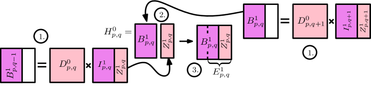
Figure 8. The reduction procedure: 1. The standard reduction into cycles and boundaries 2. Reduction of cycle basis with respect to cycle basis, the reduction proceeds left to right. Note that certain chains (non-essential classes) in $Z^{1}_{pq}$ will be completely reduced. Since these are already in the span of the chosen basis we drop those columns. 3. The input to the next iteration ignores null persistent classes (in the picture we assume they happen in a left block, but this is only for visualization).

Initialization

: The initialization corresponds to running the standard persistence algorithm on each column in the double complex with $d^{0}$. As in [8], by reducing the boundary matrix and keeping track of column operations we can extract all the required bases at each node $(p,q)$(Figure 7). We now perform one additional operation: at each node, we reduce the cycle basis with respect to the boundary basis as shown in Figure 8. We do this additional step to make operations at later stages simpler.

To keep track of the preboundary we track the operations performed to produce the non-zero reduced columns of the boundary matrix. This way, we get a minimal spanning set of $I^{1}_{p,q}$ such that $d^{0}$ yields an isomorphism $I^{1}_{p,q}\to B^{1}_{p,q-1}$. At the end of this step, we have matrices representing $Z^{1}_{p,q}$, $B^{1}_{p,q}$ and $I^{1}_{p,q}$ for all $(p,q)$. $Z^{1}_{p,q}$ and part of $B^{1}_{p,q}$ together form a basis for $E^{1}_{p,q}$. We omit the boundary elements because $E^{r}$ is a subquotient of all earlier $E^{j}$, so any non-trivial class in $E^{r}$ is represented earlier, and any relation from earlier remains a relation. Hence, any null-persistent class may show up as a relation, but only a relation killing its corresponding cycle, which also will no longer be relevant. Therefore they are still valid relations for the basis but cannot map to any element in $E^{r}_{p-r+1,q+r}$.

Iteration

: The general iteration computes the basis for $Z^{r}$, $B^{r}$, $I^{r}$, from which we compute $E^{r+1}$. Note that these do not need to be stored over multiple iterations. We store the 0-th iteration from the initialization and then only the previous iteration: For the $r$-th iteration, we only have $(r-1)$-th iteration. Once completed we can forget the $(r-1)$-th iteration. As before, we first assume that all the $r$-differentials are given as linear maps. Practically, we compute the differential from the information in each subsequent iteration. This can be thought of as a subroutine we call at the beginning of each iteration and is described below.

The rest of the iteration follows much as the initialization, we apply $d^{r}$ to $E_{p,q}^{r}$. Each element gives a chain $x\in E_{p-r+1,q+r}^{r}$. We first reduce $x$ with respect to the existing boundary chains. In Figure 9, we show how we perform a reduction step. We reduce the chain $x$ with respect to $y$. The underlying operation is the same as for regular reduction in Gaussian elimination: we multiply the pivot column with the appropriate field coefficient and add it to the chain we are reducing. The only additional book-keeping we must do is to take care that the degrees of the cycle and boundary chains are appropriately updated.

Assume that both $x$ and $y$ are inessential classes, so each has a generator and a boundary relation. To illustrate this, Figure 9 shows the mapping between two persistence interval, representing the degrees of the generators and relations. Such a mapping would generically map some interval $[c,d]$ to an interval $[a,b]$, with $a\leq c\leq b\leq d$. This corresponds to the requirement that the maps be graded so generators map to multiples of generators and relations map to relations. The kernel of the map is represented by $x$ shifted to the degree of the relation of $y$. The cokernel is represented by $y$ with the relation at the degree of the generator of $x$. The image is represented by $y$, with a degree shift up to the generator of $x$. The transformation of the intervals is shown in Figure 9.

This corresponds to only one reduction step, we repeat this procedure completely reducing $x$ in terms of the basis in $E_{p-r+1,q+r}^{r}$ and we do this for all elements in $E_{p,q}^{r}$. If in the reduction of an element, an interval is reduced to zero (i.e. $[c,c]$), further reduction is unnecessary, since it cannot be in the kernel, nor can can it map to anything further in the boundary. The kernel of the map is given by all the elements which have non-null persistence and form a basis for $Z_{p,q}^{r+1}$. Likewise, in the target space (assuming $Z_{p-r+1,q+r}^{r+1}$ had already been computed), the remaining non-null persistent classes form a basis $E_{p-r+1,q+r}^{r+1}$. We note that we can compute the basis for the boundary and kernel independently. However, then we must reduce the kernel basis with repect to the boundary basis (just as in the initialization).

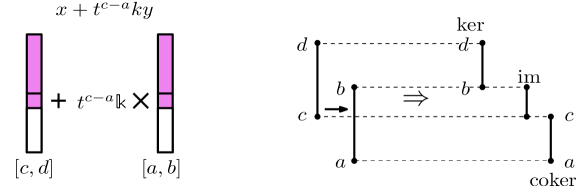
Figure 9. To perform a reduction of the $x\in d^{r}E^{r}_{p+r-1,q-r}$ with an element of the basis of $y\in E^{r}_{p,q}$, we multiply by the appropriate coefficient $t^{c-a}k\in\mathbb{k}[t]$ and add the two. The condition $a\leq c\leq b\leq d$ follows from the grading of the maps. We update the degrees of $d^{r}E^{r}_{p+r-1,q-r}$ to $[b,d]$ and $E^{r}_{p,q}$ to $[a,c]$. Note that if we get $[d,d]$ or $[a,a]$, these elements have become null persistent.

Computing the $r$-differential

: For $r=1$, the differential is given by $d^{1}$, where the map on homology is induced directly from the chain map.

For $r>1$, we use the following procedure to compute $d^{r}$ shown in Figure 10. In the previous iteration, we store the image of $d^{r-1}E^{r-1}_{p,q}$. More precisely, we store the representation of the image in the basis of $B^{0}_{p-r+2,q+r-1}$. In this basis, performing the lift to $I^{0}_{p-r+2,q+r}$ can be done through the stored relation. The lift exists because from Section 2, we know that $d^{r-1}E^{r}_{p,q}\in B^{0}_{p-r+2,q+r-1}$.

The last step is applying the $d^{1}$ map, which gives the chain we then reduce with respect to the $E^{r}_{p-r+1,q+r}$ basis. By construction this satisfies equations 2 and  3. This is precisely one step of the staircase shown in Figure 3.

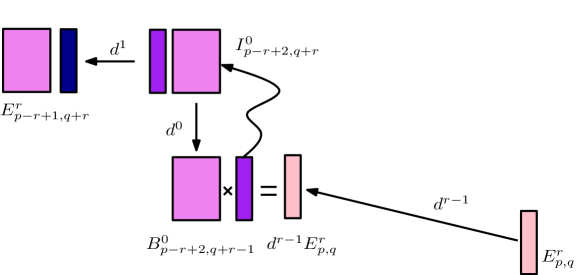
Figure 10. To compute $d^{r}$, we first find the representation of the $d^{r-1}E^{r}_{p,q}$ in terms of $B^{0}_{p-r+1,q+r-1}$. Since we know this is in the image of $d^{0}$, we can lift this vector to $I^{0}_{p-r+1,q+r}$ and then compute the chain in terms of $I^{0}_{p-r+1,q+r}$. Applying $d^{1}$, we get a chain we can reduce in terms of $E^{r}_{p-r+1,q+r}$, thereby computing $d^{r}$

References

- [1] R. Bott and L. Tu. Differential forms in algebraic topology, volume 82. Springer, 1982.
- [2] K. Brown. Cohomology of groups, volume 87 of Graduate Texts in Mathematics. Springer, 1982.
- [3] G. Carlsson. Topology and data. American Mathematical Society, 46(2):255–308, 2009.
- [4] F. Chazal and S. Y. Oudot. Towards persistence-based reconstruction in euclidean spaces. In Proc. 24th ACM Sympos. Comput. Geom., pages 232–241, 2008.
- [5] C. Chen and M. Kerber. An output-sensitive algorithm for persistent homology. In Proceedings of the 27th annual symposium on Computational geometry, 2011.
- [6] T. Chow. You could have invented spectral sequences. Notices of the AMS, 53:15–19, 2006.
- [7] D. Cohen-Steiner, H. Edelsbrunner, J. Harer, and D. Morozov. Persistent homology for kernels, images, and cokernels. In Proceedings of the twentieth Annual ACM-SIAM Symposium on Discrete Algorithms, pages 1011–1020. Society for Industrial and Applied Mathematics, 2009.
- [8] D. Cohen-Steiner, H. Edelsbrunner, and D. Morozov. Vines and vineyards by updating persistence in linear time. In Proceedings of the twenty-second annual symposium on Computational geometry, SCG ’06, pages 119–126, New York, NY, USA, 2006. ACM.
- [9] A. L. D. Attali and D. Salinas. Efficient data structure for representing and simplifying simplicial complexes in high dimension. In Proc. 27th ACM Sympos. Comput. Geom., 2011.
- [10] P. Dlotko, M. Juda, M. Mrozek, and R. Ghrist. Distributed computation of coverage in sensor networks by homological methods, 2011.
- [11] P. Dlotko, T. Kaczynski, M. Mrozek, and T. Wanner. Coreduction homology algorithm for regular cw-complexes. Discrete and Computational Geometry, 46(2):361–388, 2011.
- [12] H. Edelsbrunner and J. Harer. Computational Topology: an Introduction. AMS Press, 2009.
- [13] H. Edelsbrunner, D. Letscher, and A. Zomorodian. Topological persistence and simplification. In Foundations of Computer Science, 2000. Proceedings. 41st Annual Symposium on, pages 454–463. IEEE, 2000.
- [14] D. Eisenbud. Commutative algebra with a view toward algebraic geometry, volume 150. Springer, 1995.
- [15] R. Ghrist. Barcodes: the persistent topology of data. Bulletin-American Mathematical Society, 45(1):61, 2008.
- [16] R. Godement. Topologie algébrique et théorie des faisceaux, volume 1. Hermann Paris, 1958.
- [17] S. Harker, K. Mischaikow, M. Mrozek, V. Nanda, H. Wagner, M. Juda, and P. Dlotko. The efficiency of a homology algorithm based on discrete morse theory and coreductions. In 3rd International Workshop on Computational Topology in Image Context, November 2010.
- [18] A. Hatcher. Spectral sequences in algebraic topology. First three chapters of book in progress published online on http://www.math.cornell.edu/~hatcher/SSAT/SSATpage.html.
- [19] A. Hatcher. Algebraic topology. Cambridge University Press, 2005.
- [20] P. P. K. Mischaikow, M. Mrozek. Graph approach to the computation of the homology of continuous maps. Foundations of Computational Mathematics, 5:199–229, 2005.
- [21] J. McCleary. A user’s guide to spectral sequences, volume 58. Cambridge Univ Pr, 2001.
- [22] N. Milosavljevic, D. Morozov, P. Skraba, et al. Zigzag persistent homology in matrix multiplication time. In Annual Symposium on Computational Geometry, pages 247–256, 2009.
- [23] M. Mrozek and B. Batko. Coreduction homology algorithm. Discrete and Computational Geometry, 41:96–118, 2009.
- [24] M. Mrozek, P. Pilarczyk, and N. Zelazna. Homology algorithm based on acyclic subspace. Computers and Mathematics with Applications,, 55:2395–2412, 2008.
- [25] M. Mrozek and T. Wanner. Coreduction homology algorithm for inclusions and persistent homology. Computers and Mathematics with Applications, accepted.
- [26] A. Muhammad and A. Jadbabaie. Distributed computation of homology groups by gossip. In American Control Conference, ACC 2007, 2007.
- [27] C. Sims. Abstract algebra: a computational approach. John Wiley & Sons, Inc., 1984.
- [28] A. Zomorodian. Topology for computing. Cambridge Univ Pr, 2005.
- [29] A. Zomorodian. Fast construction of the vietoris-rips complex. Computers & Graphics, 34(3):263–271, 2010.
- [30] A. Zomorodian. The tidy set: a minimal simplicial set for computing homology of clique complexes. In Proceedings of the 2010 annual symposium on Computational geometry, pages 257–266. ACM, 2010.
- [31] A. Zomorodian and G. Carlsson. Computing persistent homology. Discrete and Computational Geometry, 33(2):249–274, 2005.
- [32] A. Zomorodian and G. Carlsson. Localized homology. In Shape Modeling and Applications, 2007. SMI’07. IEEE International Conference on, pages 189–198. IEEE, 2007.