GEF-TH 03/11

Abstract: It is shown that, under the conditions of validity of the Fresnel approximation, diffraction and interference for a monochromatic wave traveling in the $z$-direction may be described in terms of the spreading in time of the transverse ($x,y$) wave packet. The time required for the evolved wave packet to yield identical patterns as given by standard optics corresponds to the time for the quantum to cross the optical apparatus. This point of view may provide interesting cues in wave mechanics and quantum physics education.

PACS: 01.04.-d, 01.55.-b, 03.65.-w, 42.25.-p

1 Introduction

In dealing with the time evolution of free De Broglie wave packets one may wonder whether optical phenomena as diffraction or interference are related in some way to the spreading of the wave function. Consider, for instance, a plane wave traveling in the $z$-direction and impinging on a screen with a thin slit along the $y$-axis. Now think about the slit as a device preparing an “initial” wave function in the $x$-direction (see lower part of Fig. 1). This wave function will evolve to yield, at a later time $t$, a probability density distribution identical to the diffraction pattern given by classical optics on a screen at some distance $z$ from the slit (see upper part of Fig. 1).

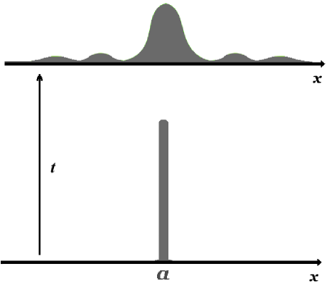
Figure 1: A rectangular wave function, as that created by a slit of width $a$, will evolve to yield, at a later time $t$, a probability distribution identical to the diffraction pattern foreseen by classical optics on a screen at some distance $z$ from the slit.

Analogous considerations are still more instructive in the case of the two-slit experiment. When the experiment is performed with particles at very low intensities (a particle at a time) [1], the interference pattern emerges collecting a large number of independent events, i.e. performing the same experiment many times under the same conditions. The wave mechanical description is simple: Just beyond the screen we get an “initial” wave function essentially given by the sum of the two peaks in correspondence of the two slits (see lower part of Fig. 2) and properly normalized to 1 (i.e. to one particle). At a later time $t$ this wave function will display a probability distribution of localization that reproduces the Young interference fringes (see upper part of Fig. 2).

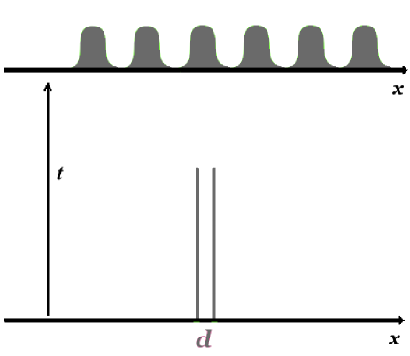
Figure 2: As in Fig.1 for a wave function sum of two real narrow peaks a distant $d$ apart. At a later time $t$ the evolved wave function yields a probability distribution that reproduces the Young interference fringes.

The relation between spreading of one-dimensional wave packets and the diffraction of light has been dealt with in [2] and recently emphasized [3] in connection with the observation of nonspreading Airy beams [4]. In fact the unusual features of these beams were predicted by Berry and Balazs [5] in the framework of one-dimensional wave mechanics. Moreover it could provide a helpful tool in teaching quantum physics, especially when facing the coherent nature of the wave function, its statistical interpretation, or the subtleties of the two-slit experiment [6].

Though useful this point of view may be, it does not seem to be exploited for educational purposes, as it can be realized by checking existing textbooks on wave mechanics. The reason, I presume, is that the issue still deserves some clarifications. For instance we should answer, in a plain way, the following naive questions: We know that the evolution of free De Broglie waves for particles of mass $m$ is driven by the dispersion relation:

$$\omega_{k}=\frac{\hbar k^{2}}{2m}$$ (1)

(where $\omega_{k}$ is the angular frequency for a wave number $k$) which follows immediately from the mechanical non-relativistic energy-momentum relation ($E=p^{2}/2m$) and the wave particle relationships: $E=\hbar\omega$ ; $p=\hbar k$. The spreading of De Broglie wave packets is known to be due to the dispersive nature of Eq. (1). How can it be that the final density distributions be identical (apart from the different scale of wave lengths) to those of non dispersive ones, like e.m.-waves propagating in vacuum? Moreover, does the above evolution time actually correspond to the time elapsed for the particle to travel from the slits to the detection screen?

In the present paper the above questions will be addressed. The time evolved transverse wave packet will be compared with the corresponding three-dimensional stationary solution derived by the method of the angular spectrum [7]. As we shall see, the key point for matching the two kinds of solution rests upon the classical Fresnel approximation. In the framework of this approximation we will find that the time required for the wave packet to reproduce the same diffraction or interference pattern as that given by the stationary wave, is $t=z/v_{g}$, where $v_{g}$ is the group velocity of the incident wave and $z$ the distance between the screen with the slits and the detection screen. This result is quite general. In the case of experiments performed with particles, we could say, using a classical language, it is exactly the time for the particle to cover that distance.

2 Evolution of De Broglie waves

In this Section we recall briefly the main equations relevant to the time evolution of free De Broglie wave packets. Throughout this paper, for simplicity, only one-dimensional wave packets will be considered, though the problem at hand applies, in general, to two-dimensional wave packets (see next Sect.).

So, let us consider a free particle of mass $m$ on the $x$-axis. If we know the wave function $\psi(x,0)$ at the time $t=0$ we get the solution of the (time-dependent) Schrödinger equation as:

$$\psi(x,t)=\frac{1}{\sqrt{2\pi}}\int_{-\infty}^{+\infty}\hat{\psi}(k)\exp[i(kx-\omega_{k}t)]dk$$ (2)

where

$$\hat{\psi}(k)=\frac{1}{\sqrt{2\pi}}\int_{-\infty}^{+\infty}\psi(x,0)\exp(-ikx)dx$$ (3)

is the Fourier Transform of the initial wave function and $\omega_{k}$ is given by Eq. (1)

We may write the solution (2) in a more compact form by introducing the propagator [8]:

$$\psi(x,t)=\sqrt{\frac{m}{2\pi i\hbar t}}\int\exp\Big{(}i\frac{m(x-x^{\prime})^{2}}{2\hbar t}\Big{)}\psi(x^{\prime},0)dx^{\prime}$$ (4)

From Eq. (4) a useful approximation may be drawn when the initial wave packet is concentrated in a small region around the origin:

$$(x-x^{\prime})^{2}\approx x^{2}-2xx^{\prime}$$ (5)

that yields:

$$|\psi(x,t)|^{2}\approx\frac{m}{2\pi\hbar t}\Big{|}\int\exp\big{(}-i\frac{mx}{\hbar t}x^{\prime}\big{)}\psi(x^{\prime},0)dx^{\prime}\Big{|}^{2}$$ (6)

In this approximation the evolved wave function is obtained by simply Fourier transforming the initial wave function.

In fact Eq. (5) will be a sensible approximation for the wave packets at hand and Eq. (6) will provide a nimble calculation.

For instance in the case of an initial wave function different from zero only in a small region of width $a$ around the origin and approximately constant therein, we get:

$$|\psi(x,t)|^{2}=|N|^{2}\Big{|}\int_{-\frac{a}{2}}^{\frac{a}{2}}\exp[-i\frac{mx}{\hbar t}x^{\prime}]dx^{\prime}\Big{|}^{2}\propto\frac{\sin^{2}(\frac{ma}{2\hbar t}x)}{(\frac{ma}{2\hbar t}x)^{2}}$$ (7)

(See Fig. 1).

While in the case of an initial wave function sum of two equal narrow peaks a small distance $d$ apart, we can roughly write:

$$\psi(x,0)=N\Big{(}\delta(x+d/2)+\delta(x-d/2)\Big{)}$$ (8)

and Eq. (6) immediately yields the probability distribution at time $t$:

$$|\psi(x,t)|^{2}=|N|^{2}\bigg{\arrowvert}\int_{-\infty}^{\infty}\exp[-i\frac{mx}{\hbar t}x^{\prime}]\psi(x^{\prime},0)dx^{\prime}\bigg{\arrowvert}^{2}\propto\cos^{2}(\frac{md}{2\hbar t}x)$$ (9)

(See Fig. 2).

3 An outline of the method of the Angular Spectrum

In this Section we address the following problem: Consider a monochromatic wave, with angular frequency $\omega_{0}$:

$$\Phi(x,y,z;t)=\phi(x,y,z)\exp[-i\omega_{0}t]$$ (10)

incident on the $xy$ plane and traveling in the positive $z$-direction. Suppose we know the spatial part of the wave function $\phi(x,y,z)$ at every point of the plane $z=0$; we want to calculate the wave function at a subsequent plane $z$.

When (10) is inserted into the wave equation, one gets the Helmholtz equation for the spatial part :

$$\Delta\phi=-k_{0}^{2}\phi$$ (11)

Note that Eq. (11) is just the same equation for different kinds of waves: Electromagnetic (when described by a scalar function), De Broglie or even Klein-Gordon waves; the differences residing in the relationships between the frequency $\omega_{0}$ and the wave number $k_{0}$:

$$\omega_{0}=\left\{\begin{array}[]{lll}ck_{0}&&\textrm{e.m.}\\ &&\\ \frac{\hbar k_{0}^{2}}{2m}&&\textrm{De Br.}\\ &&\\ \sqrt{c^{2}k_{0}^{2}+m^{2}c^{4}/\hbar^{2}}&&\textrm{Kl.-G.}\end{array}\right.$$ (12)

So, what follows will be true independently of the nature of the waves considered.

The method proceeds now by Fourier transforming $\phi(x,y,z)$ with respect to the $x,y$ coordinates. Since, as anticipated, we assume complete symmetry along the $y$-axis, we may get rid of the $y$ coordinate and perform a one-dimensional Fourier transformation:

$$\phi(x,z)=\frac{1}{\sqrt{2\pi}}\int A(k_{x},z)\exp[ik_{x}x]dk_{x}$$ (13)

Then the amplitude $A(k_{x},z)$ satisfies:

$$\frac{d^{2}}{dz^{2}}A(k_{x},z)=-(k_{0}^{2}-k_{x}^{2})A(k_{x},z)$$ (14)

whose solutions are, in general, combinations of $\exp\big{(}\pm i\sqrt{k_{0}^{2}-k_{x}^{2}}\ z\big{)}$.

However, by hypothesis, only progressive waves in the $z$-directions are allowed, so that:

$$A(k_{x},z)=A(k_{x},0)\exp\big{(}i\sqrt{k_{0}^{2}-k_{x}^{2}}\ z\big{)}$$ (15)

The amplitude $A(k_{x},0)$ is the Fourier Transform of $\phi(x,0)$:

$$A(k_{x},0)=\frac{1}{\sqrt{2\pi}}\int\phi(x,0)\exp[-ik_{x}x]dx$$ (16)

and is known as the angular spectrum of $\phi(x,0)$ [7]. So, from the knowledge of the wave function at the plane $z=0$, we get the wave function at the plane $z$:

$$\phi(x,z)=\frac{1}{\sqrt{2\pi}}\int A(k_{x},0)\exp[i(k_{x}x+\sqrt{k_{0}^{2}-k_{x}^{2}}\,z)]dk_{x}$$ (17)

Now in the usual optics experiments only small angles intervene, that means the angular spectrum $A(k_{x},0)$ is different from zero only for $k_{x}<<k_{0}$. This is the point where the Fresnel approximation comes through [7]:

$$\sqrt{k_{0}^{2}-k_{x}^{2}}\approx k_{0}-k_{x}^{2}/2k_{0}$$ (18)

So we get:

$$\phi(x,z)\approx\frac{\exp(ik_{0}z)}{\sqrt{2\pi}}\int A(k_{x},0)\exp[i(k_{x}x-\frac{k_{x}^{2}}{2k_{0}}z)]dk_{x}=$$

$$=\exp(ik_{0}z)\sqrt{\frac{k_{0}}{2\pi iz}}\int\exp\Big{(}i\frac{k_{0}}{2z}(x-x^{\prime})^{2}\Big{)}\phi(x^{\prime},0)dx^{\prime}$$ (19)

We can still go further with the Fraunhofer approximation [7]:

$$\exp\Big{(}i\frac{k_{0}}{2z}x^{\prime 2}\Big{)}\approx 1$$ (20)

to obtain

$$\phi(x,z)\propto\int\exp\Big{(}-i\frac{k_{0}x}{z}x^{\prime}\Big{)}\phi(x^{\prime},0)dx^{\prime}$$ (21)

Note that Eq. (20) is the counterpart of the approximation (5) in wave mechanics.

4 Matching the two solutions

As noted, the above equations refer to any kind of waves. For De Broglie waves we compare Eq. (4) with Eq. (19). Identifying $\psi(x,t=0)\equiv\phi(x,z=0)$ one has:

$$|\psi(x,t)|^{2}\equiv|\phi(x,z)|^{2}$$ (22)

provided that:

$$t=\frac{mz}{\hbar k_{0}}\equiv z/v_{g}$$ (23)

Eqs. (22,23) are the main result of the present paper. Since $k_{0}$ is the wave number of the incident beam, $v_{g}=\hbar k_{0}/m$ is the group velocity of the wave traveling in the $z$ direction. According to the small angles hypothesis $k_{z}\approx k_{0}$, so the time (23) actually corresponds to the time that the particle spends for traveling from the slits to the detection screen.

As a final point we will check that the same interpretation holds for non-dispersive waves as well as for relativistic particles waves.

• Electromagnetic Waves:

  The time evolution of a one-dimensional wave packet (of any kind) in a uniform medium is formally given by Eq. (2), that we rewrite here, for the sake of clarity, with the substitutions $k\rightarrow k_{x}$ and $\omega_{k}\rightarrow\omega(k_{x})$:

  $$\psi(x,t)=\frac{1}{\sqrt{2\pi}}\int_{-\infty}^{+\infty}\hat{\psi}(k_{x})\exp[i(k_{x}x-\omega(k_{x})t)]dk_{x}$$ (24)

  For De Broglie waves it was of course $\omega(k_{x})=\hbar k_{x}^{2}/2m$; for light waves, on the other hand, when the Fresnel approximation is valid (i.e. $k_{z}\approx k_{0}$) one has:

  $$\omega(k_{x})=c\sqrt{k_{z}^{2}+k_{x}^{2}}\approx ck_{0}+\frac{ck_{x}^{2}}{2k_{0}}$$ (25)

  So, looking at the dependence of $\omega$ on $k_{x}$, one sees an effective dispersion relation similar to that of De Broglie waves, with the substitution $\hbar/m\rightarrow c/k_{0}$. This means that these wave packets will spread in time, along the $x$ axis, much like De Broglie wave packets. Finally putting

  $$t=z/c$$ (26)

  in Eq. (24), since $\hat{\psi}(k_{x})\equiv A(k_{x},0)$, we recover (but a phase factor that does not change the diffraction or interference pattern) the stationary wave solution $\phi(x,z)$ Eq. (19) at the plane $z$.

• Klein-Gordon Waves:

  Here (from $E=\sqrt{p^{2}c^{2}+m^{2}c^{4}}$) we get:

  $$\omega(k_{x})=c\sqrt{k_{z}^{2}+k_{x}^{2}+m^{2}c^{2}/\hbar^{2}}\approx c\sqrt{k_{0}^{2}+m^{2}c^{2}/\hbar^{2}}+\frac{ck_{x}^{2}}{2\sqrt{k_{0}^{2}+m^{2}c^{2}/\hbar^{2}}}$$ (27)

  to be inserted into Eq. (24). In this case the matching with the stationary solution Eq. (19) is found when:

  $$t=z\frac{\sqrt{k_{0}^{2}+m^{2}c^{2}/\hbar^{2}}}{ck_{0}}=z/v_{g}$$ (28)

  In Eq. (28)

  $$v_{g}\equiv\frac{ck_{0}}{\sqrt{k_{0}^{2}+m^{2}c^{2}/\hbar^{2}}}=pc^{2}/E$$ (29)

  is the group velocity of Klein-Gordon waves (at the wave number $k_{0}$) which coincides with the velocity of a relativistic particle with momentum $p=\hbar k_{0}$.

5 Conclusions

This paper aimed at clarifying a question that may be exploited in physics education. It has been shown that, within the classical Fresnel approximation, the diffraction or interference patterns in an optical experiment may be described in terms of time evolution of the transverse wave packet. Comparing the evolved (one- or two-dimensional) wave packet at time $t$ with the corresponding “space evolved” wave function at the plane $z$, derived by the methods of Fourier optics, one gets identical patterns when $t=z/v_{g}$ where $v_{g}$ is the group velocity of the incident wave. Though the main interest was focused on De Broglie waves, this result is quite general and holds for any waves propagating in a uniform medium. In the case of optical experiments performed with particles, we could say that $t$ is the time spent by the particle to cover the distance $z$ and this is true for relativistic particles as well. This point of view may be useful, for instance, in discussing the two-slit experiment performed with single electrons.

References

- [1] P. G. Merli, G. F. Missiroli, and G. Pozzi, “On the optical aspect of electons interference phenomena”, Am. J. Phys. 44, 306-307 (1976); A. Tonomura, J. Endo, T. Kawasaki, and H. Ezawa, “Demonstration of single-electron buildup of an interference pattern”, Am. J. Phys. 57, 117-120 (1989).
- [2] G. Vandegrift, “The diffraction and spreading of a wave packet”, Am. J. Phys. 72, 404-408 (2004).
- [3] K. Dholakia, “Optics: Against the spread of light”, Nature 451, 413 (2008).
- [4] G. A. Siviloglou, J. Broky, A. Dogariu, and D. N. Christodoulides, “Observation of Accelerating Airy Beams”, Phys. Rev. Lett. 99, 213901(4) (2007).
- [5] M. V. Berry and Balazs, “Nonspreading wave packets”, Am. J. Phys. 47, 264-267 (1979).
- [6] R. P. Feynman, R. B. Leighton, and M. Sands, The Feynman Lectures on Physics (Addison-Wesley, Menlo Park, CA, 1965), Vol. III.
- [7] J. W. Goodman, Introduction to Fourier Optics (Mc Graw Hill Book Co., San Francisco, 1968).
- [8] See for instance: J. J. Sakurai, Modern Quantum Mechanics (Benjamin -Cummings, Menlo Park, CA, 1985).