On the Optimal Scheduling of Independent, Symmetric and Time-Sensitive Tasks

Abstract

Consider a discrete-time system in which a centralized controller (CC) is tasked with assigning at each time interval (or slot) $K$ resources (or servers) to $K$ out of $M\geq K$ nodes. When assigned a server, a node can execute a task. The tasks are independently generated at each node by stochastically symmetric and memoryless random processes and stored in a finite-capacity task queue. Moreover, they are time-sensitive in the sense that within each slot there is a non-zero probability that a task expires before being scheduled. The scheduling problem is tackled with the aim of maximizing the number of tasks completed over time (or the task-throughput) under the assumption that the CC has no direct access to the state of the task queues. The scheduling decisions at the CC are based on the outcomes of previous scheduling commands, and on the known statistical properties of the task generation and expiration processes.

Based on a Markovian modeling of the task generation and expiration processes, the CC scheduling problem is formulated as a partially observable Markov decision process (POMDP) that can be cast into the framework of restless multi-armed bandit (RMAB) problems. When the task queues are of capacity one, the optimality of a myopic (or greedy) policy is proved. It is also demonstrated that the MP coincides with the Whittle index policy. For task queues of arbitrary capacity instead, the myopic policy is generally suboptimal, and its performance is compared with an upper bound obtained through a relaxation of the original problem.

Overall, the settings in this paper provide a rare example where a RMAB problem can be explicitly solved, and in which the Whittle index policy is proved to be optimal.

I Introduction and System Model

The problem of scheduling concurrent tasks under resource constraints finds applications in a variety of fields including communication networks [1], distributed computing [2] and virtual machine scenarios [3]. In this paper we consider a specific instance of this general problem in which a centralized controller (CC) is tasked with assigning at each time interval (or slot) $K$ resources, referred to as servers, to $K$ out of $M\geq K$ nodes as shown in Fig. 1. A server can complete a single task per slot and can be assigned to one node per time interval. The tasks are generated at the $M$ nodes by stochastically symmetric, independent and memoryless random processes. The tasks are stored by each node in a finite-capacity task queue, and they are time-sensitive in the sense that at each slot there is a non-zero probability that a task expires before being completed successfully. It is assumed that the CC has no direct access to the node queues, and thus it is not fully informed of their actual states. Instead, the scheduling decision is based on the outcomes of previous scheduling commands, and on the statistical knowledge of the task generation and expiration processes. If a server is assigned to a node with an empty queue, it remains idle for the whole slot. The purpose here is thus to pair servers to nodes so as to maximize the average number of successfully completed tasks within either a finite or infinite number of slots (horizon), which we refer to as task-throughput, or simply throughput.

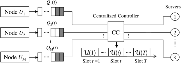
Figure 1: The centralized controller (CC) assigns $K$ resources (servers) to $K$ out of $M\geq K$ nodes to complete their tasks in each slot $t$. The tasks of node $U_{i}$ at slot $t$ are stored in a task queue $Q_{i}(t).$

I-A Markov Formulation

We now introduce the stochastic model that describes the evolution of the task queues across slots. In this section we consider task queues of capacity one (see Sec. V for capacity larger than one), where $Q_{i}(t)\in\{0,1\}$ denotes the number of tasks in the queue of node $U_{i}$, for $i\in\{1,...,M\}$. The stochastic evolution of queue $Q_{i}(t)$ is shown in Fig. 2 as a function of the scheduling decision $\mathcal{U}(t)$, which consists in the assignment at each slot $t$ of the $K$ servers to a subset $\mathcal{U}(t)\subseteq\{U_{1},...,U_{M}\}$ of $K$ nodes, with $\left|\mathcal{U}(t)\right|=K$.

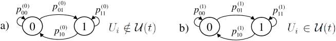
Figure 2: Markov model for the evolution of the state of the task queue $Q_{i}(t)\in\{0,1\}$, when the node $U_{i}$: a) is not scheduled in slot $t$ (i.e., $U_{i}\notin\mathcal{U}(t)$); b) is scheduled in slot $t$ (i.e., $U_{i}\in\mathcal{U}(t)$).

At each slot, node $U_{i}$ can be either scheduled ($U_{i}\in\mathcal{U}(t)$) or not ($U_{i}\notin\mathcal{U}(t)$). If $U_{i}$ is not scheduled (i.e., $U_{i}\notin\mathcal{U}(t)$, see Fig. 2-a)) and there is a task in its queue (i.e., $Q_{i}(t)=1$), then the task expires with probability (w.p.) $p_{10}^{(0)}=\Pr[Q_{i}(t+1)=0|Q_{i}(t)=1,U_{i}\notin\mathcal{U}(t)]$, while it remains in the queue w.p. $p_{11}^{(0)}=1-p_{10}^{(0)}$. Instead, if node $U_{i}$ is scheduled (i.e., $U_{i}\in\mathcal{U}(t)$, see Fig. 2-b)) and $Q_{i}(t)=1$, its task is completed successfully and its queue in the next slot is either empty or full w.p. $p_{10}^{(1)}=\Pr[Q_{i}(t+1)=0|Q_{i}(t)=1,U_{i}\in\mathcal{U}(t)]$ and $p_{11}^{(1)}=1-p_{10}^{(1)}$, respectively. Probability $p_{11}^{(1)}$ accounts for the possible arrival of a new task. If $Q_{i}(t)=0$ the probabilities of receiving a new task when $U_{i}$ is not scheduled and scheduled are $p_{01}^{(0)}=\Pr[Q_{i}(t+1)=1|Q_{i}(t)=0,U_{i}\notin\mathcal{U}(t)]$ and $p_{01}^{(1)}=\Pr[Q_{i}(t+1)=1|Q_{i}(t)=0,U_{i}\in\mathcal{U}(t)]$, respectively, while the probabilities of receiving no task are $p_{00}^{(0)}=1-p_{01}^{(0)}$ and $p_{00}^{(1)}=1-p_{01}^{(1)}$, respectively.

I-B Related Work and Contributions

In this work we assume that the CC has no direct access to the state of the task queues $Q_{1}(t),...,Q_{M}(t)$, while it knows the transitions probabilities $p_{xy}^{(u)}$, with $x,y,u\in\{0,1\}$, and the outcomes of previously scheduled tasks. The scheduling problem is thus formalized as a partially observable Markov decision process (POMDP) [4], and then cast into a restless multi-armed bandit (RMAB) problem [5]. A RMAB is constituted by a set of arms (the queues in our model), a subset of which needs to be activated (or scheduled) in each slot by the controller.

To elaborate, we assume that the transition probabilities of the Markov chains in Fig. 2, the number of nodes $M$ and servers $K$ are such that

$$m=M/K,\text{ }\text{is integer, and}$$ (1a)

$$p_{11}^{(1)}\leq p_{01}^{(1)}\leq p_{01}^{(0)}\leq p_{11}^{(0)}.$$ (1b)

Assumption (1a) states that the ratio $m=M/K$ between the numbers $M$ of nodes and $K$ of servers is an integer, generalizing the single-server case ($K=1$). Proving the results provided later in this paper for the case of non-integer $m$ remains an open problem. Assumption (1b) is motivated as follows. The inequality $p_{11}^{(1)}\leq p_{01}^{(1)}$ imposes that the probability that a new task arrives when the task queue is full and the node is scheduled ($p_{11}^{(1)}$) is no larger than when the task queue is empty ($p_{01}^{(1)}$). This applies, e.g., when the arrival of a new task is independent on the queue’s state and scheduling decisions (i.e., $p_{11}^{(1)}=p_{01}^{(1)}$), or when a new task is not accepted when the queue is full, i.e., $p_{11}^{(1)}=0$. Inequality $p_{01}^{(1)}\leq p_{01}^{(0)}$ applies, e.g., when the task generation process does not depend on the queue’s state and on the scheduling decisions, so that $p_{01}^{(1)}=p_{01}^{(0)}$, or when a new task cannot be accepted while the node is scheduled even if the queue is empty ($p_{01}^{(1)}=0$). Inequality $p_{01}^{(0)}\leq p_{11}^{(0)}$ indicates that, when a node is not scheduled, the probability $p_{01}^{(0)}$ that its task queue is full in the next slot, given that it is currently empty, is smaller than the probability $p_{11}^{(0)}$ that the task queue is full in the next slot given that it is currently full. This applies, e.g., when the task generation and expiration processes are independent of each other.

Main Contributions: When the task queues are of capacity one, and under assumptions (1), we first show that the myopic policy (MP) for the RMAB at hand is a round robin (RR) strategy that: i) re-numbers the nodes in a decreasing order according to the initial probability that their respective task queue is full; and then ii) schedules the nodes periodically in group of $K$ by exploiting the initial ordering. The MP is then proved to be throughput-optimal. We then show that, for the special case in which $p_{01}^{(0)}=p_{01}^{(1)}$ and $p_{10}^{(0)}=p_{11}^{(1)}=0$, the MP coincides with the Whittle index policy, which is a generally suboptimal index strategy for RMAB problems [6]. Finally, we extend the model of Sec. I-A to queues with an arbitrary capacity $C$. Characterizing optimal policies for $C>1$ is significantly more complicated than the case of $C=1$. Hence, inspired by the optimality of the MP for $C=1$, we compare the performance of the MP for $C>1$, with a upper bound based on a relaxation of the scheduling constraints of the original RMAB problem [6]. It is recalled that the results in this paper represent a rare case in which the optimal policy for a RMAB can be found explicitly [5].

Related Work: The work in this paper is related to the works [7, 8], in which a RMAB problem similar to the one in this paper is addressed. However, the main difference between our RMAB and the one in [7, 8] is the evolution of the arms across slots. In particular, in our RMAB, each arm evolves across a slot depending on the scheduling decision taken by the controller, while in [7, 8], the evolution of the arms does not depend on the scheduling decision. The transition probabilities for the RMAB in [7, 8] are thus equivalent to setting $p_{01}^{(0)}=p_{01}^{(1)}$ and $p_{11}^{(0)}=p_{11}^{(1)}$ in the Markov chains of Fig. 2. For instance, our model applies to scenarios in which the arms are, e.g., data queues, where each arm draws a data packet from its queue only when scheduled. Instead, the model in [7, 8] applies to scenarios in which the arms are, e.g., communication channels, whose quality evolves across slots regardless whether they are selected for transmission or not.

In [7] it is shown that the MP is optimal for $p_{01}^{(0)}=p_{01}^{(1)}\leq p_{11}^{(0)}=p_{11}^{(1)}$ with $K=1,$ while [8] extends this result to an arbitrary $K.$ The work [7] also demonstrates that the MP in not generally optimal in the case $p_{01}^{(0)}=p_{01}^{(1)}\geq p_{11}^{(0)}=p_{11}^{(1)}$. Finally, paper [9] proves the optimality of the Whittle index policy for $p_{11}^{(0)}=p_{11}^{(1)}\leq p_{11}^{(0)}=p_{11}^{(1)}.$ We emphasize that neither our model nor the one considered in [7, 8] subsumes the other, and the results here and in the mentioned previous works should be considered as complementary.

Notation: Vectors are denoted in bold, while the corresponding non-bold letters denote the vectors components. Given a vector $\mathbf{x=[}x_{1},...,x_{M}\mathbf{]}$ and a set $\mathcal{S=}\left\{i_{1},...,i_{K}\right\}\subseteq\left\{1,...,M\right\}$ of cardinality $K\leq M\mathbf{,}$ we define vector $\mathbf{x}_{\mathcal{S}}=[x_{i_{1}},...,x_{i_{K}}]$, where $i_{1}\leq...\leq i_{K}$. A function $f(\mathbf{x})$ of vector $\mathbf{x}$ is also denoted as $f(x_{1},...,x_{M})$ or as $f(x_{1},...,x_{l},\mathbf{x}_{\{l+1,...,M\}})$ for some $1\leq l\leq M$, or similar notations depending on the context. Given a set $\mathcal{A}$ and a subset $\mathcal{B\subseteq A},$ $\mathcal{B}^{c}$ represents the complement of $\mathcal{B}$ in $\mathcal{A}$.

II Problem Formulation

Here we formalize the scheduling problem of Sec. I (see Fig. 1), in which the task generation and expiration processes are modeled, independently at each node, by the Markov models of Sec. I-A with queues of capacity one. Extension to task queues of arbitrary capacity is addressed in Sec. V.

II-A Problem Definition

The scheduling problem at the CC is addressed in a finite-horizon scenario over slots $t\in\{1,...,T\}$. Let $\mathbf{Q}(t)=\left[Q_{1}(t),...,Q_{M}(t)\right]$ be the vector collecting the states of the task queue at slot $t$. At slot $t=1,$ the CC is only aware of the initial probability distribution $\boldsymbol{\omega}(1)=[\omega_{1}(1),...,\omega_{M}(1)]$ of $\mathbf{Q}(1)$, whose $i$th entry is $\omega_{i}(1)=\Pr[Q_{i}(1)=1]$. Thus, the subset $\mathcal{U}(1)$ of $\left|\mathcal{U}(1)\right|=K$ nodes scheduled at slot $t=1$ is chosen as a function of the initial distribution $\boldsymbol{\omega}(1)$ only. For any node $U_{i}\in\mathcal{U}(t)$ scheduled at slot $t$, an observation is made available to the CC at the end of the slot, while no observations are available for non-scheduled nodes $U_{i}\notin\mathcal{U}(t)$. Specifically, if $Q_{i}(t)=1$ and $U_{i}\in\mathcal{U}(t)$, the task of $U_{i}$ is served within slot $t$, and the CC observes that $Q_{i}(t)=1$. Conversely, if $Q_{i}(t)=0$ and $U_{i}\in\mathcal{U}(t)$, no tasks are completed and the CC observes that $Q_{i}(t)=0$. We define $\mathcal{O}(t)=\left\{Q_{i}(t):\>U_{i}\in\mathcal{U}(t)\right\}$ as the set of (new) observations available at the CC at the end of slot $t$. At time $t,$ the CC hence knows the history of all decisions and previous observations and the initial distribution $\boldsymbol{\omega}(1)$, namely $\mathcal{H}(t)=\left\{\mathcal{U}(1),...,\mathcal{U}(t-1),\mathcal{O}(1),...,\mathcal{O}(t-1),\boldsymbol{\omega}(1)\right\}$, with $\mathcal{H}(1)=\left\{\boldsymbol{\omega}(1)\right\}$.

Since the CC has only partial information about the system state $\mathbf{Q}(t)$, through $\mathcal{O}(t)$, the scheduling problem at hand can be modeled as a POMDP. It is well-known that a sufficient statistics for taking decisions in such POMDP is given by the probability distribution of $\mathbf{Q}(t)$ conditioned on the history $\mathcal{H}(t)$ [10], referred to as belief, and represented by the vector $\boldsymbol{\omega}(t)=[\omega_{1}(t),...,\omega_{M}(t)]$, with $i$th entry given by

$$\omega_{i}(t)=\Pr\left[Q_{i}(t)=1|\mathcal{H}(t)\right].$$ (2)

Since the belief $\boldsymbol{\omega}(t)$ fully summarizes the entire history $\mathcal{H}(t)$ of past actions and observations [10], a scheduling policy $\pi\mathbf{=}\left[\mathcal{U}^{\pi}(1),...,\mathcal{U}^{\pi}(T)\right]$ is defined as a collection of functions $\mathcal{U}^{\pi}(t)$ that map the belief $\boldsymbol{\omega}(t)$ to a subset $\mathcal{U}(t)$ of $\left|\mathcal{U}(t)\right|=K$ nodes, i.e., $\mathcal{U}^{\pi}(t)$: $\boldsymbol{\omega}(t)\rightarrow\mathcal{U}(t)$. We will refer to $\mathcal{U}^{\pi}(t)$ as the subset of scheduled nodes, even though, strictly speaking, it is the mapping function defined above. The transition probabilities over the belief space are derived in Sec. II-B.

The immediate reward $R(\boldsymbol{\omega},\mathcal{U})$, accrued by the CC when the belief vector is $\boldsymbol{\omega}$ and action $\mathcal{U}$ is taken, measures the average number of tasks completed within the current slot, and it is

$$R(\mathbf{\boldsymbol{\omega}},\mathcal{U})=\sum_{U_{i}\in\mathcal{U}}\omega_{i}.$$ (3)

Notice that $R(\mathbf{\boldsymbol{\omega}},\mathcal{U})\leq K$ since there are only $K$ servers.

The throughput measures the average number of tasks completed over the slots $\{1,...,T\}$ that, by exploiting (3) and under policy $\pi$, is given by

$$V_{1}^{\pi}\left(\mathbf{\boldsymbol{\omega}}(1)\right)=\sum_{t=1}^{T}\beta^{t-1}\mathrm{E}^{\mathbf{\pi}}\left[R\left(\mathbf{\boldsymbol{\omega}}(t)\mathbf{,}\mathcal{U}^{\mathbf{\pi}}(t)\right)|\mathbf{\boldsymbol{\omega}}(1)\right].$$ (4)

In (4), the expectation $\mathrm{E}^{\mathbf{\pi}}[\cdot|\mathbf{\boldsymbol{\omega}}(1)]$, under policy $\pi$ for initial belief $\mathbf{\boldsymbol{\omega}}(1)$, is intended with respect to the distribution of the Markov process $\mathbf{\boldsymbol{\omega}}(t)$, as obtained from the transition probabilities to be derived in Sec. II-B. For generality, the definition (4) includes a discount factor $0\leq\beta\leq 1$ [7], while the infinite horizon scenario (i.e., $T\rightarrow\infty$) will be discussed in Sec. III-C.

The goal is to find a policy $\pi^{\ast}=\left[\mathcal{U}^{*}(1),...,\mathcal{U}^{*}(T)\right]$ that maximizes the throughput (4) so that

$$V_{1}^{\mathbf{\ast}}\left(\boldsymbol{\omega}(1)\right)=V_{1}^{\pi^{\ast}}\left(\boldsymbol{\omega}(1)\right)=\underset{\pi}{\max}V_{1}^{\pi}\left(\boldsymbol{\omega}(1)\right), \pi^{\ast}=\arg\max_{\pi}V_{1}^{\pi}\left(\boldsymbol{\omega}(1)\right)$$ with (5)

II-B Transition Probabilities

The belief transition probabilities, given decision $\mathcal{\mathcal{U}}(t)=\mathcal{\mathcal{U}}$ and $\boldsymbol{\omega}(t)=\boldsymbol{\omega}=[\omega_{1},...,\omega_{M}]$, are

$$p_{\boldsymbol{\omega\omega^{\prime}}}^{(\mathcal{U})}=\Pr\left[\boldsymbol{\omega}(t+1)=\boldsymbol{\omega}^{\prime}|\boldsymbol{\omega}(t)=\boldsymbol{\omega},\mathcal{\mathcal{U}}(t)=\mathcal{\mathcal{U}}\right]=\prod\limits_{i=1}^{M}\Pr[\omega_{i}(t+1)=\omega_{i}^{\prime}|\omega_{i}(t)=\omega_{i},\mathcal{\mathcal{U}}(t)=\mathcal{\mathcal{U}}],$$ (6)

where $\boldsymbol{\omega}(t+1)=\boldsymbol{\omega}^{\prime}=[\omega^{\prime}_{1},...,\omega^{\prime}_{M}]$, while the distribution of entry $\omega_{i}(t+1)$ is (see Fig. 2)

$$\Pr[\omega_{i}(t+1)=\omega_{i}^{\prime}|\omega_{i}(t)=\omega_{i},\mathcal{\mathcal{U}}(t)=\mathcal{\mathcal{U}}]=\left\{\begin{array}[]{ll}\omega_{i}&\text{if }\omega_{i}^{\prime}=p_{11}^{(1)}\textrm{ and }U_{i}\in\mathcal{U}\\ \left(1-\omega_{i}\right)&\text{if }\omega_{i}^{\prime}=p_{01}^{(1)}\textrm{ and }U_{i}\in\mathcal{U}\\ 1&\text{if }\omega_{i}^{\prime}=\tau_{0}^{(1)}(\omega_{i})\textrm{ and }U_{i}\notin\mathcal{U}\end{array}\right.,$$ (7)

where we have defined the deterministic function

$$\tau_{0}^{(1)}(\omega) = \Pr[Q_{i}(t+1)=1|\omega_{i}(t)=\omega,U_{i}\notin\mathcal{U}(t)]=\omega p_{11}^{(0)}+(1-\omega)p_{01}^{(0)}=\omega\delta_{0}+p_{01}^{(0)}$$ (8)

to indicate the next slot’s belief when $U_{i}$ is not scheduled ($U_{i}\notin\mathcal{U}(t)$), with $\delta_{0}=p_{11}^{(0)}-p_{01}^{(0)}\geq 0$ due to inequalities (1b). Eq. (8) follows from Fig. 2-a), since the next slot’s belief is either $p_{11}^{(0)}$ if $Q_{i}(t)=1$ (w.p. $\omega$) or $p_{01}^{(0)}$ if $Q_{i}(t)=0$ (w.p. $\left(1-\omega\right)$). A generalization of function $\tau_{0}^{(1)}(\omega)$ that computes the belief $\omega_{i}(t+k)$ of node $U_{i}$ when it is not scheduled for $k$ successive slots, e.g., slots $\{t,...,t+k-1\},$ and $\omega_{i}(t)=\omega$, can be obtained as

$$\tau_{0}^{(k)}(\omega)=\Pr[B_{i}(t+k)=1|\omega_{i}(t)=\omega,U_{i}\notin\mathcal{U}(t),...,U_{i}\notin\mathcal{U}(t+k-1)]=\omega\delta_{0}^{k}+p_{01}^{(0)}\frac{1-\delta_{0}^{k}}{1-\delta_{0}}.$$ (9)

Eq. (9) can be obtained recursively from (8) as $\tau_{0}^{(k)}(\omega)=\tau_{0}^{(1)}(\tau_{0}^{(k-1)}(\omega))$, for all $k\geq 1$, with $\tau_{0}^{(0)}(\omega)=\omega$.

Under assumptions (1b), it is easy to verify that function (8) satisfies the inequalities

$$p_{11}^{(1)}\leq p_{01}^{(1)}\leq\tau_{0}^{(1)}(\omega)\text{, for all }0\leq\omega\leq 1,\textrm{ and}$$ (10)

$$\tau_{0}^{(1)}(\omega)\leq\tau_{0}^{(1)}(\omega^{\prime})\text{, for all }\omega\leq\omega^{\prime}\text{ with }0\leq\omega,\omega^{\prime}\leq 1.$$ (11)

The inequalities in (10) guarantee that the belief of a non-scheduled node is always larger than that of a scheduled one, while the inequality (11) says that the belief ordering of two non-scheduled nodes is maintained across a slot. These inequalities play a crucial role in the analysis below.

II-C Optimality Equations

The dynamic programming (DP) formulation of problem (5) (see e.g., [11]) allows to express the throughput recursively over the horizon $\{t,...,T\}$, under policy $\pi$ and initial belief $\boldsymbol{\omega}$, as

$$V_{t}^{\pi}(\boldsymbol{\omega}) =\sum_{j=t}^{T}\beta^{j-t}\mathrm{E}^{\mathbf{\pi}}\left[R\left(\boldsymbol{\omega}(j)\mathbf{,}\mathcal{U}^{\mathbf{\pi}}(j)\right)|\boldsymbol{\omega}(t)=\boldsymbol{\omega}\right]=R\left(\boldsymbol{\omega}\mathbf{,}\mathcal{U}^{\mathbf{\pi}}(t)\right)+\beta\sum_{\mathbf{\omega}^{\prime}}p_{\boldsymbol{\omega\omega}^{\prime}}^{(\mathcal{U}^{\pi})}V_{t+1}^{\pi}(\boldsymbol{\omega}^{\prime}),$$ (12)

where $V_{t}^{\pi}(\cdot)=0$ for $t>T$. The DP optimality conditions (or Bellman equations) are then expressed in terms of the value function $V_{t}^{\ast}(\boldsymbol{\omega})=\max_{\pi}V_{t}^{\pi}(\boldsymbol{\omega})$, which represents the optimal throughput in the interval $\{t,...,T\}$, and it is given by

$$V_{t}^{\ast}(\boldsymbol{\omega}) = \underset{\mathcal{U}(t)=\mathcal{U}\subseteq\{U_{1},...,U_{M}\}}{\max}\left\{R(\mathbf{\boldsymbol{\omega}},\mathcal{U})+\beta\sum_{\mathbf{\omega}^{\prime}}p_{\boldsymbol{\omega\omega}^{\prime}}^{(\mathcal{U})}V_{t+1}^{*}(\boldsymbol{\omega}^{\prime})\right\}.$$ (13)

Note that, since the nodes are stochastically equivalent, the value function (13) only depends on the numerical values of the entries of the belief vector $\boldsymbol{\omega}$ regardless of the way it is ordered. Finally, an optimal policy $\pi^{\ast}=\left[\mathcal{U}^{\ast}(1),...,\mathcal{U}^{\ast}(T)\right]$ (see (5)) is such that $\mathcal{U}^{\ast}(t)$ attains the maximum in the condition (13) for $t\in\{1,2,...,T\}$.

III Optimality of the Myopic Policy

We now define the myopic policy (MP) and show that, under assumptions (1), it is a round-robin (RR) policy that schedules the nodes periodically and that it is optimal for problem (5).

III-A The Myopic Policy is Round-Robin

The MP $\pi^{MP}=\{\mathcal{U}^{MP}(1),...,\mathcal{U}^{MP}(T)\}$, with throughput $V_{t}^{MP}(\cdot)$, is the greedy policy that schedules at each slot the $K$ nodes with the largest beliefs so as to maximize the immediate reward (3), that is, we have

$$\mathcal{U}^{MP}(t) =\arg\max_{\mathcal{U}}R(\mathbf{\boldsymbol{\omega}}(t),\mathcal{U})=\arg\max_{\mathcal{U}}\sum_{U_{i}\in\mathcal{U}}\omega_{i}(t).$$ (14)

Proposition 1.

Under assumptions (1), the MP (14), given an initial belief $\boldsymbol{\omega}^{\prime}(1)$, is a RR policy that operates as follows: 1) Sort vector $\boldsymbol{\omega}^{\prime}(1)$ in a decreasing order to obtain $\boldsymbol{\omega}(1)=\left[\omega_{1}(1),...,\omega_{M}(1)\right]$ such that $\omega_{1}(1)\geq...\geq\omega_{M}(1)$. Re-number the nodes so that $U_{i}$ has belief $\omega_{i}(1)$; 2) Divide the nodes into $m$ groups of $K$ nodes each, so that the $g$th group $\mathcal{G}_{g}$, $g\in\{1,...,m\}$, contains all nodes $U_{i}$ such that $g=\left\lfloor\frac{i-1}{K}\right\rfloor+1$, namely: $\mathcal{G}_{1}=\{U_{1},...,U_{K}\},$ $\mathcal{G}_{2}=\{U_{K+1},...,U_{2K}\},$ and so on; 3) Schedule the groups in a RR fashion with period $m$ slots, so that groups $\mathcal{G}_{1},...,\mathcal{G}_{m},\mathcal{G}_{1},...$ are sequentially scheduled at slot $t=1,...,m,m+1,...$ and so on.

Proof:

According to (14), the first scheduled set is $\mathcal{U}^{MP}(1)$ $=\mathcal{G}_{1}=\{U_{1},U_{2},...,U_{K}\}$. The beliefs are then updated through (7). Recalling (10), the scheduled nodes, in $\mathcal{G}_{1}$, have their belief updated to either $p_{11}^{(1)}$ or $p_{01}^{(1)}$, which are both smaller than the belief of any non-scheduled node in $\{U_{1},...,U_{M}\}\setminus\mathcal{G}_{1}$. Moreover, the ordering of the non-scheduled nodes’ beliefs is preserved due to (11). Hence, the second scheduled group is $\mathcal{U}^{MP}(2)$ $=\mathcal{G}_{2}$, the third is $\mathcal{U}^{MP}(3)$ $=\mathcal{G}_{3},$ and so on. This proves that the MP, upon an initial ordering of the beliefs, is a RR policy. ∎

We emphasize that the MP sorts the beliefs of the nodes only at the first slot in which it is operated, and then it keeps scheduling the groups of nodes according to their initial ordering, without requiring to recalculate the beliefs.

III-B Optimality of the Myopic Policy

We now prove the optimality of the MP by showing that it satisfies the Bellman equations (13). To start with, let us consider a RR policy $\pi^{RR}$ that operates according to steps 2) and 3) of Proposition 1 (i.e., without re-ordering the initial belief), and let its throughput (12) be denoted by $V_{t}^{RR}(\mathbf{\boldsymbol{\omega}})$. Note that, when the initial belief $\boldsymbol{\omega}$ is ordered so that $\omega_{1}\geq...\geq\omega_{M}$, then $V_{t}^{RR}(\boldsymbol{\omega})=V_{t}^{MP}(\boldsymbol{\omega})$. Based on backward induction arguments similarly to [7, 8], the following lemma establishes a sufficient condition for the optimality of the MP.

Lemma 2.

Assume that the MP is optimal at slot $t+1,...,T$, i.e., it satisfies (13). To show that the MP is optimal also at slot $t$ it is sufficient to prove the inequality

$$V_{t}^{RR}(\boldsymbol{\omega}_{\mathcal{S}},\boldsymbol{\omega}_{\mathcal{S}^{c}})\leq V_{t}^{MP}(\boldsymbol{\omega}_{\mathcal{S}},\boldsymbol{\omega}_{\mathcal{S}^{c}})=V_{t}^{RR}(\omega_{1},\omega_{2},...,\omega_{M}),\quad\textrm{for all }\omega_{1}\geq\omega_{2}\geq...\geq\omega_{M}$$ (15)

and all sets $\mathcal{S}\subseteq\{1,...,M\}$ of $K$ elements, with the elements in $\boldsymbol{\omega}_{\mathcal{S}^{c}}$ decreasingly ordered.

Proof:

Since the MP is optimal from $t+1$ onward by assumption, it is sufficient to show that scheduling $K$ nodes with arbitrary beliefs at slot $t$ and then following the MP from slot $t+1$ on is no better than following the MP immediately at slot $t$. The performance of the former policy is given by the left-hand side (LHS) of (15). In fact $V_{t}^{RR}(\boldsymbol{\omega}_{\mathcal{S}},\boldsymbol{\omega}_{\mathcal{S}^{c}})$, for any set $\mathcal{S}$, represents the throughput of a policy that schedules the $K$ nodes with beliefs $\boldsymbol{\omega}_{\mathcal{S}}$ at slot $t$, and then operates as the MP from $t+1$ onward, since beliefs in $\boldsymbol{\omega}_{\mathcal{S}^{c}}$ are decreasingly ordered. The MP’s performance is instead given by the right-hand side (RHS) of (15). Note that, for $t=T$, it is immediate to verify that the MP is optimal. This concludes the proof.∎

Theorem 3.

Under assumptions (1) the MP is optimal for problem (5), so that $\pi^{MP}=\pi^{\ast}$.

Proof:

To start with, we first prove in Appendix A that the inequality

$$V_{t}^{RR}(\omega_{1},...,\omega_{j},y,x,...,\omega_{M}) \leq V_{t}^{RR}(\omega_{1},...,\omega_{j},x,y,...,\omega_{M})$$ (16)

holds for any $x\geq y$, with $0\leq j\leq M-2$, and for all $t\in\{1,...,T\}$ and beliefs $\omega_{k}$ (not necessarily ordered), with $k\in\{1,...,M\}$. Inequality (16) for $j=0$ is intended as $V_{t}^{RR}(y,x,...,\omega_{M})\leq V_{t}^{RR}(x,y,...,\omega_{M})$. If (16) holds, then inequality (15) is satisfied for all $\omega_{1}\geq...\geq\omega_{M}$ and all subsets $\mathcal{S}\subseteq\{1,...,M\}$ of $K$ elements. In fact, (16) states that the throughput of the RR policy never increases when, for any pair of adjacent nodes, the one with the smallest belief of the pair is scheduled first. Hence, by starting from the RHS of (15) (i.e., $V_{t}^{RR}(\omega_{1},\omega_{2},...,\omega_{M})$) and by applying a convenient number of successive switchings between pair of adjacent elements of vector $[\omega_{1},\omega_{2},...,\omega_{M}]$ to achieve $[\boldsymbol{\omega}_{\mathcal{S}},\boldsymbol{\omega}_{\mathcal{S}^{c}}]$, for any $\mathcal{S}$, we can obtain a cascade of inequalities through (16) (one for each switching), which guarantees that (15) holds. By Lemma 2 this is sufficient to prove that the MP is optimal, since the inequality (15) holds for any arbitrary $t$. ∎

III-C Extension to the Infinite-Horizon Case

We now briefly describe the extension of problem (5) to the infinite-horizon case, for which the throughput under policy $\pi$ and its optimal value are given by (see e.g., [7])

$$V^{\pi}\left(\mathbf{\boldsymbol{\omega}}(1)\right)=\sum_{t=1}^{\infty}\beta^{t-1}\mathrm{E}^{\mathbf{\pi}}\left[R\left(\mathbf{\boldsymbol{\omega}}(t)\mathbf{,}\mathcal{U}^{\pi}(t)\right)|\mathbf{\boldsymbol{\omega}}(1)\right], V^{\ast}\left(\mathbf{\boldsymbol{\omega}}(1)\right)=\max_{\pi}V^{\pi}\left(\mathbf{\boldsymbol{\omega}}(1)\right),$$ and (17)

where the optimal policy is $\pi^{\ast}=\arg\max_{\pi}V^{\pi}\left(\mathbf{\boldsymbol{\omega}}(1)\right)$ and $0\leq\beta<1$. From standard DP theory [11], the optimal policy $\pi^{\ast}$ is stationary, so that the optimal decision $\mathcal{U}^{*}(t)$ is a function of the current state $\mathbf{\omega}(t)$ only, independently of slot $t$ [11]. By following the same reasoning as in [7, Theorem 3], it can be shown that the optimality of the MP for the finite-horizon setting implies the optimality also for the infinite-horizon scenario. Moreover, by following [7, Theorem 4] it can be shown that the MP is optimal also for the undiscounted average reward criterion (i.e., $V_{avg}^{\pi}\left(\mathbf{\boldsymbol{\omega}}(1)\right)=lim_{T\rightarrow\infty}\frac{1}{T}\sum_{t=1}^{\infty}\mathrm{E}^{\mathbf{\pi}}\left[R\left(\mathbf{\boldsymbol{\omega}}(t)\mathbf{,}\mathcal{U}^{\pi}(t)\right)|\mathbf{\boldsymbol{\omega}}(1)\right]$).

IV Optimality of the Whittle Index Policy

In this section, we briefly review the Whittle index policy for RMAB problems [5], and then focus on the infinite-horizon scenario of Sec. III-C, when conditions (1b) are specialized to

$$0=p_{11}^{(1)}\leq p_{01}^{(1)}=p_{01}^{(0)}=p_{01}\leq p_{11}^{(0)}=1,$$ (18)

and where the task queues are of capacity one. We show that under the assumption (18) (see Sec. I-B for a discussion on these conditions), the RMAB at hand is indexable and we calculate its Whittle index in closed-form. We then show that the Whittle index policy is equivalent to the MP, and thus optimal for the problem (17).

We emphasize that, our results provide a rare example [5] in which, as in [9], not only indexability is established, but also the Whittle index is obtained in closed form and the Whittle policy proved to be optimal. It is finally remarked that our proof technique is inspired by [9], but the different system model poses new challenges that require significant work.

IV-A Whittle Index

The Whittle index policy assigns a numerical value $W(\omega_{i})$ to each state $\omega_{i}$ of node $U_{i}$, referred to as index, to measure how rewarding it is to schedule node $U_{i}$ in the current slot. The $K$ nodes with the largest index are then scheduled in each slot. As detailed below, the Whittle index is calculated independently for each node, and thus the Whittle index policy is not generally optimal for RMAB problems. Moreover, even the existence of a well-defined Whittle index is not guaranteed [5]. To study the indexability and the Whittle index for the RMAB at hand, we can focus on a restless single-armed bandit (RSAB) model, as defined below [5]. A RSAB is a RMAB with a single arm, in which the only decision that needs to be taken by the CC is whether activating the (single) arm or not (i.e., keep it passive).

IV-A1 RSAB with Subsidy for Passivity

The Whittle index is based on the concept of subsidy for passivity, whereby the CC is given a subsidy $m\in\mathbb{R}$ when the arm is not scheduled. At each slot $t$, the CC, based on the state $\omega(t)$ of the arm, can decide to activate (or schedule) it, i.e., to set $u(t)=1$, obtaining an immediate reward $R_{m}(\omega(t),1)=\omega(t)$. If, instead, the arm is kept passive, i.e., $u(t)=0$, a reward $R_{m}(\omega(t),0)=m$ equal to the subsidy is accrued. The state $\omega(t)$ evolves through (7), which under (18) and adapted to the simplified notation used here becomes

$$\omega(t+1)=\left\{\begin{array}[]{llc}0&\text{w.p. }\omega(t)&\text{if }u(t)=1\\ p_{01}&\text{w.p. }\left(1-\omega(t)\right)&\text{if }u(t)=1\\ \tau_{0}^{(1)}(\omega(t))&\text{w.p. }1&\text{if }u(t)=0\end{array}\right..$$ (19)

The throughput, given policy $\pi=\left\{u^{\pi}(1),u^{\pi}(2),...\right\}$ and initial belief $\omega(1)$, is

$$V_{m}^{\pi}\left(\omega(1)\right)=\sum_{t=1}^{\infty}\beta^{t-1}\mathrm{E}^{\pi}\left[R_{m}(\omega(t),u^{\pi}(t))|\omega(1)\right].$$ (20)

The optimal throughput is $V_{m}^{\ast}\left(\omega(1)\right)=\max_{\pi}V_{m}^{\pi}\left(\omega(1)\right)$, while the optimal policy
$\pi^{\ast}=\arg\max_{\pi}V_{m}^{\pi}\left(\omega(1)\right)$ is stationary in the sense that the optimal decisions $u_{m}^{\ast}(\omega)\in\{0,1\}$ are functions of the belief $\omega$ only, independently of slot $t$ [9]. Removing the slot index from the initial belief, the optimal throughput $V_{m}^{\ast}\left(\omega\right)$ and the optimal decision $u_{m}^{\ast}(\omega)$ satisfy the following DP optimality equations for the infinite-horizon scenario (see [9])

$$V_{m}^{\ast}(\omega) = \underset{u\in\{0,1\}}{\max}\left\{V_{m}(\omega|u)\right\},$$ (21)

$$\textrm{and }u_{m}^{\ast}(\omega) = \arg\underset{u\in\{0,1\}}{\max}\left\{V_{m}(\omega|u)\right\}.$$ (22)

In (21)-(22) we defined $V_{m}(\omega|u),$ $u\in\{0,1\}$, as the throughput (20) of a policy that takes action $u$ at the current slot and then uses the optimal policy $u_{m}^{\ast}\left(\omega\right)$ onward, we have

$$V_{m}(\omega|0) = m+\beta V_{m}^{\ast}(\tau_{0}^{(1)}\left(\omega\right)),\textrm{ {and}}$$ (23)

$$V_{m}(\omega|1) = \omega+\beta\left[\omega V_{m}^{\ast}(0)+(1-\omega)V_{m}^{\ast}(p_{01})\right].$$ (24)

IV-A2 Indexability and Whittle Index

We use the notation of [9] to define indexability and Whittle index for the RSAB at hand. We first define the so called passive set

$$\mathcal{P}(m)=\left\{\omega\text{: }0\leq\omega\leq 1\text{ and }u_{m}^{\ast}(\omega)=0\right\},$$ (25)

as the set that contains all the beliefs $\omega$ for which the passive action is optimal (i.e., all $0\leq\omega\leq 1$ such that $V_{m}(\omega|0)\geq V_{m}(\omega|1)$, see (23)-(24)) under the given subsidy for passivity $m\in\mathbb{R}$. The RMAB at hand is said to be indexable if the passive set $\mathcal{P}(m)$, for the associated RSAB problem, is monotonically increasing as $m$ increases within the interval $(-\infty,+\infty),$ in the sense that $\mathcal{P}(m^{\prime})\subseteq$ $\mathcal{P}(m)$ if $m^{\prime}\leq m$ and $\mathcal{P}(-\infty)=\emptyset$ and $\mathcal{P}(+\infty)=[0,1]$.

If the RMAB is indexable, the Whittle index $W(\omega)$ for each arm with state $\omega$ is the infimum subsidy $m$ such that it is optimal to make the arm passive. Equivalently, the Whittle index $W(\omega)$ is the infimum subsidy $m$ that makes passive and active actions equally rewarding, i.e.,

$$W(\omega) = \inf\left\{m\text{: }u_{m}^{\ast}(\omega)=0\right\}=\inf\left\{m\text{: }V_{m}\left(\omega|0\right)=V_{m}\left(\omega|1\right)\right\}.$$ (26)

IV-B Optimality of the Threshold Policy

Here, we show that the optimal policy $u_{m}^{\ast}(\omega)$ for the RSAB of Sec. IV-A1 is a threshold policy over the belief $\omega$. This is crucial in our proof of indexability of the RMAB at hand given in Sec. IV-D. To this end, we observe that: i) function $V_{m}(\omega|1)$ in (24) is linear over the belief $\omega$; ii) function $V_{m}(\omega|0)=m+\beta V_{m}^{\ast}(\tau_{0}^{(1)}\left(\omega\right))$ in (23) is convex over $\omega$, since the value function $V_{m}^{\ast}(\omega)$ is convex for the problem at hand (see [9, 10]). We need the following lemma.

Lemma 4.

The following inequalities hold:

a) For $$0\leq m<1: \mathcal{\textrm{a.1) }}V_{m}(0|1)\leq V_{m}(0|0)\leq V_{m}(1|1);\quad\mathcal{\textrm{a.2) }}V_{m}(1|0)\leq V_{m}(1|1);$$ (27a)

b) For $$m<0: \mathcal{\textrm{b.1) }}V_{m}(0|0)\leq V_{m}(0|1)\leq V_{m}(1|1);\quad\mathcal{\textrm{b.2) }}V_{m}(1|0)\leq V_{m}(1|1);$$ (27b)

c) For $$m\geq 1: \mathcal{\textrm{c.1) }}V_{m}(0|0)\leq V_{m}(1|1)\leq V_{m}(0|1);\quad\mathcal{\textrm{c.2) }}V_{m}(1|1)\leq V_{m}(1|0).$$ (27c)

Proof:

See Appendix B. ∎

Leveraging Lemma 4, we can now establish the optimality of a threshold policy $u_{m}^{\ast}(\omega)$.

Proposition 5.

The optimal policy $u_{m}^{\ast}(\omega)$ in (22) for subsidy $m\in\mathbb{R}$ is given by

$$u_{m}^{\ast}(\omega)=\left\{\begin{array}[]{cc}1,&\text{if }\omega>\omega^{\ast}(m)\\ 0,&\text{if }\omega\leq\omega^{\ast}(m)\end{array}\right.,$$ (28)

where $\omega^{\ast}(m)\in\mathbb{R}$ is the optimal threshold for a given subsidy $m$. The optimal threshold $\omega^{\ast}(m)$ is $0\leq\omega^{\ast}(m)\leq 1$ if $0\leq m<1$, while it is arbitrary negative for $m<0$ and arbitrary greater than unity for $m\geq 1$. In other words we have $u_{m}^{\ast}(\omega)=1$ if $m<0$ and $u_{m}^{\ast}(\omega)=0$ if $m\geq 1$.

Proof:

We start by showing that (28), for $0\leq m<1$, satisfies (22) and is thus an optimal policy. To see this, we refer to Fig. 3, where we sketch functions $V_{m}(\omega|1)$ and $V_{m}(\omega|0)$ for different values of the subsidy $m$. From (22), we have that $u_{m}^{\ast}(\omega)=1$ for all $\omega$ such that $V_{m}(\omega|1)>V_{m}(\omega|0)$ and $u_{m}^{\ast}(\omega)=0$ otherwise. For $0\leq m<1$, from the inequalities of Lemma 4-a), the linearity of $V_{m}(\omega|1)$ and the convexity of $V_{m}(\omega|0)$, it follows that there is only one intersection $\omega^{\ast}(m)$ between $V_{m}(\omega|1)$ and $V_{m}(\omega|0)$ with $0\leq\omega^{\ast}(m)\leq 1$, as shown in Fig. 3-a). Instead, when $m<0$, by Lemma 4-b), arm activation is always optimal, that is, $u_{m}^{\ast}(\omega)=1$, since $V_{m}(\omega|1)>V_{m}(\omega|0)$ for any $0\leq\omega\leq 1$ as shown in Fig. 3-b). Conversely, when $m\geq 1$, by Lemma 4-c), it follows that passivity is always optimal, that is, $u_{m}^{\ast}(\omega)=0$, since $V_{m}(\omega|0)\geq V_{m}(\omega|1)$ for any $0\leq\omega\leq 1$ as shown in Fig. 3-c). ∎

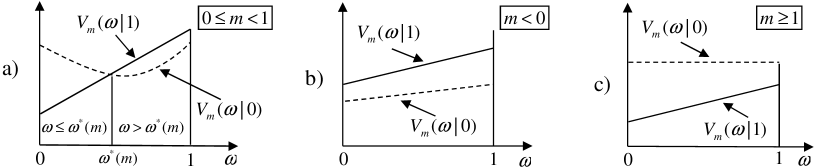
Figure 3: Illustration of the optimality of a threshold policy for different values of the subsidy for passivity $m$: a) $0\leq m<1$; b) $m<0$; c) $m\geq 1$.

IV-C Closed-Form Expression of the Value Function

By leveraging the optimality of the threshold policy (28) we derive a closed-form expression of $V_{m}^{\ast}(\omega)$ in (21), being a key step in establishing the RMAB’s indexability in Sec. IV-D.

Notice that function $\tau_{0}^{(k)}(\omega)$ in (9), when specialized to conditions (18), becomes

$$\tau_{0}^{(k)}(\omega)=1-(1-p_{01})^{k}(1-\omega),$$ (29)

which is a monotonically increasing function of $k$, so that $\tau_{0}^{(k)}(\omega)\geq\tau_{0}^{(i)}(\omega)$ for any $k\geq i$. Based on such monotonicity, we can define the average number $L(\omega,\omega^{\prime})$ of slots it takes for the belief to become larger than $\omega^{\prime}$ when starting from $\omega$ while the arm is kept passive, as

$$L(\omega,\omega^{\prime}) =\min\left\{k\text{: }\tau_{0}^{\left(k\right)}(\omega)>\omega^{\prime}\right\} =\left\{\begin{array}[]{lc}0&\omega>\omega^{\prime}\\ \left\lfloor\frac{\ln\left(\frac{1-\omega^{\prime}}{1-\omega}\right)}{\ln\left(1-p_{01}\right)}\right\rfloor+1&\omega\leq\omega^{\prime}\\ \infty&\omega\leq 1\leq\omega^{\prime}\end{array}\right..$$ (33)

From (33) we have $L(\omega,\omega^{\prime})=1$ for $\omega=\omega^{\prime}$ since, without loss of optimality, we assumed that the passive action is optimal (i.e., $u_{m}^{\ast}(\omega)=0$) when $V_{m}(\omega|0)=V_{m}(\omega|1)$. For $\omega^{\prime}\geq 1$ instead (according to Proposition 5), the arm is always kept passive and thus $L(\omega,\omega^{\prime})=\infty$.

Lemma 6.

The optimal throughput $V_{m}^{\ast}(\omega)$ in (21) can be written as

$$V_{m}^{\ast}(\omega)=\frac{1-\beta^{L(\omega,\omega^{\ast}(m))}}{1-\beta}m+\beta^{L(\omega,\omega^{\ast}(m))}V_{m}(\tau_{0}^{\left(L(\omega,\omega^{\ast}(m))\right)}(\omega)|1),$$ (34)

where $\omega^{\ast}(m)$ is the optimal threshold obtained from Proposition 5.

Proof:

According to Proposition 5, the optimal policy $u_{m}^{\ast}(\omega)$ keeps the arm passive as long as the current belief is $\omega\leq\omega^{\ast}(m)$. Therefore, the arm is kept passive for $L(\omega,\omega^{\ast}(m))$ slots, during which a reward $R_{m}(\omega,0)=m$ is accrued in each slot. This leads to a total reward within the passivity time given by the following geometric series $\sum_{k=0}^{L(\omega,\omega^{\ast}(m))-1}\beta^{k}m=\frac{1-\beta^{L(\omega,\omega^{\ast}(m))}}{1-\beta}m$, which corresponds to the first term in the RHS of (34). After $L(\omega,\omega^{\ast}(m))$ slots of passivity, the belief becomes larger than the threshold $\omega^{\ast}(m)$ and the arm is activated. The contribution to the value function $V(\omega)$ thus becomes $\beta^{L(\omega,\omega^{\ast}(m))}V_{m}(\tau_{0}^{\left(L(\omega,\omega^{\ast}(m))\right)}(\omega)|1)$, which is the second term in the RHS of (34). Note that, when $\omega>\omega^{\ast}(m)$, activation is optimal, and $V^{\ast}(\omega)=V(\omega|1)$. ∎

To evaluate $V_{m}^{\ast}(\omega)$ from (34), we only need to calculate $V_{m}(\omega|1)$ since the other terms, thanks to (33) are explicitly given once $\omega^{\ast}(m)$ is obtained from Proposition 5. However, from (24), evaluating $V_{m}(\omega|1)$ only requires $V_{m}^{\ast}(0)$ and $V_{m}^{\ast}(p_{01})$, which are calculated in the lemma below.

Lemma 7.

We have

$$V_{m}^{\ast}(0)=\frac{\left(m-2m\beta^{L_{m}^{\ast}}+\beta^{L_{m}^{\ast}}\upsilon_{m}^{\ast}-\beta^{L_{m}^{\ast}+1}\upsilon_{m}^{\ast}+m\beta^{L_{m}^{\ast}+1}+m\beta^{L_{m}^{\ast}}\upsilon_{m}^{\ast}-m\beta^{L_{m}^{\ast}+1}\upsilon_{m}^{\ast}\right)}{\left(\beta-1\right)\left(\beta^{L_{m}^{\ast}}-\beta^{L_{m}^{\ast}}\upsilon_{m}^{\ast}+\beta^{L_{m}^{\ast}+1}\upsilon_{m}^{\ast}-1\right)}$$ (35a)

$$V_{m}^{\ast}(p_{01})=\frac{\left(m\beta-m\beta^{L_{m}^{\ast}}+\beta^{L_{m}^{\ast}}\upsilon_{m}^{\ast}-\beta^{L_{m}^{\ast}+1}\upsilon_{m}^{\ast}+m\beta^{L_{m}^{\ast}+1}\upsilon_{m}^{\ast}-m\beta^{L_{m}^{\ast}+2}\upsilon_{m}^{\ast}\right)}{\beta\left(\beta-1\right)\left(\beta^{L_{m}^{\ast}}-\beta^{L_{m}^{\ast}}\upsilon_{m}^{\ast}+\beta^{L_{m}^{\ast}+1}\upsilon_{m}^{\ast}-1\right)}$$ (35b)

where we have defined $L_{m}^{\ast}=L(0,\omega^{\ast}(m))$ and $\upsilon_{m}^{\ast}=\tau_{0}^{\left(L(0,\omega^{\ast}(m))\right)}(0).$

Proof:

By plugging (24) into (34), and evaluating (34) for $\omega=0$ and $\omega=p_{01},$ we get a linear system in the two unknowns $V_{m}^{\ast}(0)$ and $V_{m}^{\ast}(p_{01})$, which can be solved leading to (35). ∎

IV-D Indexability and Whittle Index

Here, we prove that the RMAB at hand is indexable, we derive the Whittle index in closed form and show that it is equivalent to the MP and thus optimal for the RMAB problem (17).

Theorem 8.

a) The RMAB at hand is indexable and b) its Whittle index is

$$W(\omega)=\frac{\left(1-\beta^{L(0,\omega)}\left(1-\beta\tau_{0}^{L(0,\omega)}(0)\left(1-\beta\right)\left(1-h\right)\right)\right)\omega+\beta^{L(0,\omega)}\tau_{0}^{L(0,\omega)}(0)\left(1-\beta\right)\left(h\beta+1\right)}{(\beta-1)\left(\beta^{L(0,\omega)}\left(1-\beta(1-h)\right)\omega-\left(1+\beta^{L(0,\omega)}\left(\tau_{0}^{L(0,\omega)}(0)(1-\beta)+h\beta\right)\right)\right)}.$$ (36)

Proof:

Part a). See Appendix C. Part b). By (26), the Whittle index $W(\omega)$ of state $\omega$ is the value of the subsidy $m$ for which activating or not the arm is equally rewarding so that $V_{m}\left(\omega|0\right)=V_{m}\left(\omega|1\right)$. By using (23)-(24) this becomes $\omega+\beta\left[\omega V_{m}^{\ast}(0)+(1-\omega)V_{m}^{\ast}(p_{01})\right]=m+\beta V_{m}^{\ast}(\tau_{0}^{(1)}\left(\omega\right)).$ Moreover, since the threshold policy is optimal and $\tau_{0}^{(1)}\left(\omega\right)>\omega$, it follows that, when the belief becomes $\tau_{0}^{(1)}\left(\omega\right)$, it is optimal to activate the arm and thus $V_{m}^{\ast}(\tau_{0}^{(1)}\left(\omega\right))$ $=V_{m}(\tau_{0}^{(1)}\left(\omega\right)|1)=\beta\tau_{0}^{(1)}(\omega)V_{m}^{\ast}(0)+\beta(1-\tau_{0}^{(1)}(\omega))V_{m}^{\ast}(p_{01})$. Plugging this result into $V_{m}\left(\omega|0\right)=V_{m}\left(\omega|1\right)$, along with (35a) and (35b), leads to (36), which concludes the proof. ∎

It can be show that the Whittle index $W(\omega)$ in (36) is an increasing function of $\omega.$ Therefore, since the Whittle policy selects the $K$ arms with the largest index at each slot, we have:

Corollary 9.

The Whittle index policy is equivalent to the MP and is thus optimal.

V Extension to Task Queues of Arbitrary Capacity $C>1$

The problem of characterizing the optimal policies when $C>1$ is significantly more complicated than for $C=1$ and is left open by this work. Moreover, since the dimension of the state space of the belief MDP grows with $C$, even the numerical computation of the optimal policies is quite cumbersome. Due to these difficulties, here we compare the performance of the MP, inspired by its optimality for $C=1$, with a performance upper bound obtained following the relaxation approach of [6].

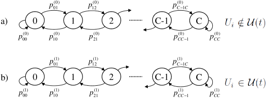
Figure 4: Markov model for the evolution of the queue $Q_{i}(t)$, of arbitrary capacity $C$, when the node $U_{i}$: a) is not scheduled in slot $t$ (i.e., $U_{i}\notin\mathcal{U}(t)$); b) is scheduled in slot $t$ (i.e., $U_{i}\in\mathcal{U}(t)$).

V-A System Model and Myopic Policy

Each node $U_{i}$ has a task queue $Q_{i}(t)\in\{0,1,...,C\}$ of capacity $C$. We consider the Markov model of Fig. 4 for the task generation and expiration processes at each node (cf. Sec. I-A). The transition probabilities between queue states when node $U_{i}$ is not scheduled are $p_{xy}^{(0)}=\textrm{Pr}[Q_{i}(t+1)=y|Q_{i}(t)=x,U_{i}\notin\mathcal{U}(t)]$, whereas when $U_{i}$ is scheduled we have $p_{xy}^{(1)}=\textrm{Pr}[Q_{i}(t+1)=y|Q_{i}(t)=x,U_{i}\in\mathcal{U}(t)]$, for $x,y\in\{0,1,...,C\}$. When node $U_{i}$ is scheduled at slot $t$, and $Q_{i}(t)\geq 1$, one of its task is executed and it also informs the CC about the number of tasks left in the queue (observation). We assume that at most one task can be generated (or dropped) in a slot, so that $p_{xy}^{(u)}=0$ for $y<x-1$ and $y>x+1$, with $u\in\{0,1\}$ as shown in Fig. 4.

The belief of each $i$th node is represented by a $\left(C\times 1\right)$ vector $\boldsymbol{\omega}_{i}=\left[\omega_{i,0},...,\omega_{i,C-1}\right]$ whose $k$th entry $\omega_{i,k}$, for $k\in\{0,1,...,C-1\}$, is given by (cf. (2)) $\omega_{i,k}=\textrm{Pr}\left[Q_{i}(t)=k|\mathcal{H}(t)\right].$ The immediate reward (3), given the initial belief vectors $\boldsymbol{\omega}_{1}(t),...,\boldsymbol{\omega}_{M}(t)$ and action $\mathcal{U}$, becomes

$$R(\boldsymbol{\omega}_{1}(t),...,\boldsymbol{\omega}_{M}(t),\mathcal{U}) = \sum_{i=1}^{M}\textrm{Pr}\left[Q_{i}(t)>0|\mathcal{H}(t)\right]1(U_{i}\in\mathcal{U})=K-\sum_{i\in\mathcal{U}}\omega_{i,0}(t).$$ (37)

The performance of interest is the infinite-horizon throughput (17).

V-A1 Myopic Policy

The MP (14), specialized to the immediate reward (37), becomes

$$\mathcal{U}^{MP}(t) = \textrm{arg}\underset{\mathcal{U}}{\textrm{max}}R(\boldsymbol{\omega}_{1}(t),...,\boldsymbol{\omega}_{M}(t),\mathcal{U})=\textrm{arg}\underset{\mathcal{U}}{\textrm{min}}\sum_{i\in\mathcal{U}}\omega_{i,0}(t).$$ (38)

Note that, unlike Sec. III-A, when $C>1$ the MP does not generally have a RR structure.

V-B Upper Bound

Here we derive an upper bound to the throughput (17) by following the approach for general RMAB problems proposed in [6]. The upper bound relaxes the constraint that exactly $K$ nodes must be scheduled in each slot. Specifically, it allows a variable number $K^{\pi}(t)$ of scheduled nodes in each $t$th slot under policy $\pi$, with the only constraint that its discounted average satisfies

$$E^{\pi}\left[\sum_{t=1}^{\infty}\beta^{t-1}K^{\pi}(t)\right]=\frac{K}{1-\beta}.$$ (39)

The advantage of this relaxed version of the scheduling problem is that it can be tackled by focusing on each single arm independently from the others [6, 12]. This is because, by the symmetry of the nodes, the constraint (39) can be equivalently handled by imposing that each node is active on average for a discounted time $E^{\pi}[\sum_{t=1}^{\infty}\beta^{t-1}1(U_{i}\in\mathcal{U}^{\pi}(t))]=\frac{K}{M(1-\beta)}$. We can thus calculate the optimal solution of the relaxed problem by solving a single RSAB problem.

We now elaborate on such a RSAB by dropping the node index. Here, the immediate reward when the arm is in state $\boldsymbol{\omega}$ (a vector since $C>1$, see Sec. V-A), and action $u\in\{0,1\}$ is chosen, is $R(\boldsymbol{\omega},u)=1-\omega_{0}$ if $u=1$ and $R(\boldsymbol{\omega},u)=0$ if $u=0$, while the Markov evolution of the belief follows from Fig. 4 and similarly to Sec. I-A. The problem consists in optimizing the throughput under the constraint $E^{\pi}[\sum_{t=1}^{\infty}\beta^{t-1}1(U_{i}\in\mathcal{U}^{\pi}(t))]=\sum_{t=1}^{\infty}\beta^{t-1}E^{\pi}[u^{\pi}(t)]=K/(M(1-\beta))$, as introduced above. Under the assumption that the state $\boldsymbol{\omega}$ belongs to a finite state space $\mathcal{W}$ (to be discussed below), this optimization can be done by resorting to a linear programming (LP) formulation [12]. Specifically, let $z_{\boldsymbol{\omega}}^{(u)}$ be the probability of being in state $\boldsymbol{\omega}$ and selecting action $u\in\{0,1\}$ under a given policy. The optimization at hand leads to the following LP

maximize $$\sum_{\boldsymbol{\omega},u} R(\boldsymbol{\omega},u)z_{\boldsymbol{\omega}}^{(u)},$$ (40a)

$$\textrm{subject to}:\;\sum_{\boldsymbol{\omega},u}z_{\boldsymbol{\omega}}^{(u)} = 1,$$ (40b)

$$\sum_{\boldsymbol{\omega}}z_{\boldsymbol{\omega}}^{(1)} = \frac{K}{M(1-\beta)},$$ (40c)

$$z_{\boldsymbol{\omega}}^{(0)}+z_{\boldsymbol{\omega}}^{(1)} = \delta\left(\boldsymbol{\omega}-\boldsymbol{\omega}(1)\right)+\beta\sum_{\boldsymbol{\omega}^{\prime},u}z_{\boldsymbol{\omega^{\prime}}}^{(u)}p_{\boldsymbol{\omega}\boldsymbol{\omega}^{\prime}}^{(u)}\textrm{, for all }\boldsymbol{\omega\in}\mathcal{W},$$ (40d)

where (40c) is the constraint on the average time in which the node is scheduled, while (40d) guarantees that $z_{\boldsymbol{\omega}}^{(u)}$ is the stationary distribution [12], in which $\delta\left(\boldsymbol{\omega}-\boldsymbol{\omega}(1)\right)=1$ if $\boldsymbol{\omega}=\boldsymbol{\omega}(1)$ and $\delta\left(\boldsymbol{\omega}-\boldsymbol{\omega}(1)\right)=0$ if $\boldsymbol{\omega}\neq\boldsymbol{\omega}(1)$ . Note that, as discussed in Sec. II, the term $p_{\boldsymbol{\omega}\boldsymbol{\omega}^{\prime}}^{(u)}$ is the probability that the next state is $\boldsymbol{\omega}^{\prime}$ given that action $u$ is taken in state $\boldsymbol{\omega}$.

We are left to discuss the cardinality of the set $\mathcal{W}$. While the belief $\boldsymbol{\omega}$ can generally assume any value in the $C$-dimensional probability simplex, the number of states actually assumed by $\omega$ during any limited horizon of time is finite due to the finiteness of the action space [10]. In our problem, since the time horizon is unlimited, this fact alone is not sufficient to conclude that the set $\mathcal{W}$ is finite. However, after each $t$th slot in which the arm is activated, the belief at the $(t+1)$th slot can only takes $C$ values given that the queue state is learned by the CC. Therefore, the evolution of the belief is reset after each activation, and in practice, the time between two activations is finite since the node must be kept active for a discounted fraction of time $K/\left(M(1-\beta\right)$. Hence, by constraining the maximum time interval between two activations to a sufficiently large value, the state space $\mathcal{W}$ remains finite and the optimal performance is not affected. We used this approach for the numerical evaluation of the upper bound in Sec. V-C.

V-C Numerical Results

We now present some numerical results to compare the performance of the MP with the upper bound of Sec. V-B. The performance is the throughput (17) normalized by its ideal value $K/\left(1-\beta\right)$ that is obtained if the nodes always have a task to be completed when scheduled.

In Fig. 5 we show the normalized throughput versus the queue capacity $C$ for different ratio $M/K$ between the number $M$ of nodes and the number $K$ of nodes scheduled in each slot. We keep $K=3$ fixed and vary $M$. We assume a uniform distribution for the initial number of tasks in the queues $Q_{i}(1)$ for all the nodes, so that $\omega_{i,k}(1)=1/\left(C+1\right)$ for all $i,k$. The probabilities that a new task is generated when the arm is kept passive are $p_{01}^{(0)}=0.15$ and $p_{kk+1}^{(0)}=0.1$, for $k\in\{1,C-1\}$, while under activation they are $p_{01}^{(1)}=0.05$ and $p_{kk+1}^{(1)}=0$. The probability that a task expires when the arm is kept passive and activated are $p_{kk-1}^{(0)}=0.05$ and $p_{kk-1}^{(1)}=0.95$ respectively. The remaining transitions probabilities are $p_{CC}^{(0)}=0.9$, $p_{CC}^{(1)}=0.05$, while $\beta=0.95$.

From Fig. 5 it can be seen that when $C$ and/or $M/K$ are small the MP’s performance is close to the upper bound. In fact, for small $M/K$, most of the nodes are scheduled in each slot and the relaxed system in Sec. V-B approaches the original one, while for small $C$ we get closer to the optimality of the MP for $C=1$. For moderate to large values of $M/K$ and/or $C$ instead, the more flexibility in the relaxed system enables larger gains over the MP.

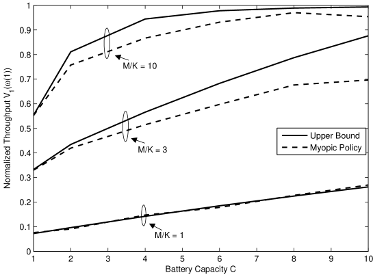
Figure 5: Normalized optimal throughput of the MP in (38) as compared to the upper bound versus the queue capacity $C$ for different ratios $M/K\in\{1,3,10\}$ (system parameters are $K=3$, $\beta=0.95$, $\omega_{i,k}(1)=1/(C+1)$ for all $i,k$, $p_{01}^{(0)}=0.15$, $p_{01}^{(1)}=0.05$, $p_{CC}^{(0)}=0.9$, $p_{CC}^{(1)}=0.05$, $p_{kk-1}^{(0)}=0.05$, $p_{kk-1}^{(1)}=0.95$, $p_{kk+1}^{(0)}=0.1$, $p_{kk+1}^{(1)}=0$, for $k\in\{1,C-1\}$).

VI Conclusions

This paper considers a centralized scheduling problem for independent, symmetric and time-sensitive tasks under resources constraints. The problem is to assign a finite number of resources to a larger number of nodes that may have tasks to be completed in their task queue. It is assumed that the central controller has no direct access to the queue of each node. Based on a Markovian modeling of the task generation and expiration processes, the scheduling problem is formulated as a partially observable Markov decision process (POMDP) and then cast into the framework of restless multi-armed bandit (RMAB) problems. Under the assumption that the task queues are of capacity one, a greedy, or myopic policy (MP), operating in the space of the a posteriori probabilities (beliefs) of the number of tasks in the queues, is proved to be optimal, under appropriate assumptions, for both finite and infinite-horizon throughput criteria. The MP selects at each slot the nodes with the largest probability of having a task to be completed. It is shown that the MP is round-robin since it schedules the nodes periodically. We have also established that the RMAB problem at hand is indexable, derived the Whittle index in closed form and shown that the Whittle index policy is equivalent to the MP and thus it is optimal.

Systems in which the task queues have arbitrary capacities have been investigated as well by comparing the performance of the MP, which is generally suboptimal, with an upper bound based on a relaxation of the scheduling constraint.

Overall, this paper proposes a general framework for resource allocation that finds applications in several areas of current interest including communication networks and distributed computing.

Appendix A Proof of Theorem 3

The proof is divided into two steps. In the first step we derive the throughput of the RR policy in closed form, and then we show that inequality (16) holds.

As for the first step, the throughput for the RR policy (and thus of the MP) can be calculated as the sum of the contribution of each node separately (due to the round robin structure). To elaborate, let us focus on node $U_{i}$, with initial belief $\omega_{i}(1)$, and assume that $U_{i}\in\mathcal{G}_{1}$. Nodes in group $\mathcal{G}_{1}$ are scheduled at slots $t\in\{1+(j-1)m\}$, for $j\in\{1,2,...\}$. Let $r_{j}(\omega_{i}(1))=\mathrm{E^{RR}}[\omega_{i}(1+(j-1)m)|\omega_{i}(1)]$ be the average reward accrued by the CC from node $U_{i}$ only, when scheduling it for the $j$th time at slot $t=1+(j-1)m$ (see the RHS of (3)) (i.e., when operating the RR policy). At slot $t=1$ we have $r_{1}(\omega_{i}(1))=\omega_{i}(1)$. To calculate $r_{2}(\omega_{i}(1))$ we first derive the average value of the belief (see (7)) after the slot of activity in $t=1$ as $\mathrm{E^{RR}}[\omega_{i}(2)|\omega_{i}(1)]=\tau_{1}^{(1)}(\omega_{i}(1))$, where $\tau_{1}^{(1)}=\omega\delta_{1}+p_{01}^{(1)}$ with $\delta_{u}=\left(p_{11}^{(u)}-p_{01}^{(u)}\right)$ (cf. (8)). We then account for the $(m-1)$ slots of passivity by exploiting (8), so that $r_{2}(\omega_{i}(1))=\mathrm{E^{RR}}[\omega_{i}(1+m)|\omega_{i}(1)]=\phi^{(1)}(\omega_{i}(t))$, where we have set $\phi^{(1)}(\omega)=\tau_{0}^{(m-1)}(\tau_{1}^{(1)}(\omega))=\omega\alpha_{m}+\psi_{m}$ with $\alpha_{m}=\delta_{1}\delta_{0}^{m-1}$ and $\psi_{m}=p_{01}^{(1)}\delta_{0}^{m-1}+p_{01}^{(0)}\frac{1-\delta_{0}^{m-1}}{1-\delta_{0}}$, and where $\tau_{0}^{(k)}(\omega)=\tau_{0}^{(1)}(\tau_{0}^{(k-1)}(\omega))$ indicates the belief of a node after $k$ slots of passivity when the initial belief is $\omega$ (i.e., $\tau_{0}^{(k)}(\omega)$ is obtained recursively by applying $\tau_{0}^{(1)}(\omega)$ to itself $k$ times). In general, we can obtain $r_{j}(\omega_{i}(1))\mathrm{=E^{RR}}[\omega_{i}(1+(j-1)m)|\omega_{i}(1)]$, for $j\geq 2$, by iterating the procedure above by applying $\phi^{(1)}(\omega)$ to itself $(j-1)$ times. After a little algebra we get $\phi^{(j-1)}(\omega)=\phi^{(1)}(\phi^{(j-2)}(\omega))=\omega\alpha_{m}^{j-1}+\psi_{m}\frac{1-\alpha_{m}^{j-1}}{1-\alpha_{m}}$, so that $r_{j}(\omega_{i}(1))=\phi^{\left(j-1\right)}(\omega_{i}(1))$, where we set $\phi^{(0)}(\omega)=\omega$. The reasoning above can be applied when starting from any arbitrary slot $t$.

Finally, the total reward accrued by the CC from a node that is scheduled $H$ times, when its belief at the first slot in which it is scheduled is $\omega$, can be calculated by summing up the average reward $r_{j}(\cdot)$ during each slot in which the node is scheduled (see definition above), as

$$\theta^{(H)}\left(\omega\right)=\sum_{j=1}^{H}\beta^{(j-1)m}r_{j}(\omega)=\frac{\psi_{m}}{1-\alpha_{m}}\left(\frac{1-\beta^{mH}}{1-\beta^{m}}-\frac{1-\left(\beta^{m}\alpha_{m}\right)^{H}}{1-\beta^{m}\alpha_{m}}\right)+\frac{1-\left(\beta^{m}\alpha_{m}\right)^{H}}{1-\beta^{m}\alpha_{m}}\omega.$$ (41)

Note that, for a node $U_{i}\in\mathcal{G}_{g}$, for $g\geq 1$ and with belief equal to $\omega$ at $t=1$, the first slot in which the node is scheduled is $t=g$ , and thus its belief at time $t=g$ becomes $\tau_{0}^{\left(g-1\right)}\left(\omega\right)$ (i.e., after $\left(g-1\right)$ slots of passivity while other groups are scheduled). Therefore, for a node $U_{i}\in\mathcal{G}_{g}$, with initial belief $\omega$, the total contribution to the throughput is given by $\beta^{g-1}\theta^{(H)}\left(\tau_{0}^{\left(g-1\right)}\left(\omega\right)\right)$.

Let us now focus on the second step, i.e., proving the inequality (16). At $t=T$, it is easily seen to hold due to (3) and (12). We then need to show that (16) also holds at $t$. To do so, let us denote as $\mathcal{L}$ and $\mathcal{R}$ the RR policies whose throughputs are given by the LHS and RHS of (16) respectively. The differences between $\mathcal{L}$ and $\mathcal{R}$ are the positions of the nodes with belief $x$ and $y$ in the initial belief vectors. Therefore, some of the $m$ groups created by the two policies might have different nodes (see the RR operations in Proposition 1). To simplify, we refer to the node with belief $x$ ($y$) as node $x$ ($y$). Let us assume that nodes $x$ and $y$ belong to groups $\mathcal{G}_{g^{\prime}}$ and $\mathcal{G}_{g^{\prime\prime}}$ under policy $\mathcal{R}$, respectively, while they belong to groups $\mathcal{G}_{g^{\prime\prime}}$ and $\mathcal{G}_{g^{\prime}}$ under policy $\mathcal{L}$, respectively, with $g^{\prime\prime}\geq g^{\prime}$, and $g^{\prime},\>g^{\prime\prime}\in\{1,...,m\}$. If $g^{\prime\prime}=g^{\prime}$, then the two policies coincide and (16) holds with equality. If $g^{\prime\prime}=g^{\prime}+1$ (nodes are adjacent but do not belong to the same group), the only difference between policies $\mathcal{L}$ and $\mathcal{R}$ is the scheduling order of nodes $x$ and $y$.

To verify that inequality (16) holds, we need to prove that scheduling node $y$ in group $\mathcal{G}_{g^{\prime}}$ and node $x$ in group $\mathcal{G}_{g^{\prime\prime}}$ is no better than doing the opposite for any $x\geq y$. To elaborate, let $H_{x}^{\mathcal{R}}(t)=H_{y}^{\mathcal{L}}(t)$ and $H_{y}^{\mathcal{R}}(t)$ $=H_{x}^{\mathcal{L}}(t)$ be the number of times that node $x$ (or $y$) is scheduled under policy $\mathcal{R}$ (or $\mathcal{L}$) and node $y$ (or $x$) is scheduled under policy $\mathcal{L}$ (or $\mathcal{R}$) in the horizon $\{t,t+1,...,T\}$, respectively. By recalling (41) and the discount factor $\beta$, the contribution generated by node $x$ and $y$ under policy $\mathcal{R}$ is $\beta^{g^{\prime}-1}\theta^{\left(H_{x}^{\mathcal{R}}(t)\right)}(\tau_{0}^{(g^{\prime}-1)}(x))$ and $\beta^{g^{\prime\prime}-1}\theta^{\left(H_{y}^{\mathcal{R}}(t)\right)}(\tau_{0}^{(g^{\prime\prime}-1)}(y))$ respectively, and similarly under policy $\mathcal{L}$ we have $\beta^{g^{\prime\prime}-1}\theta^{\left(H_{x}^{\mathcal{L}}(t)\right)}(\tau_{0}^{(g^{\prime\prime}-1)}(x))$ and $\beta^{g^{\prime}-1}\theta^{\left(H_{y}^{\mathcal{L}}(t)\right)}(\tau_{0}^{(g^{\prime}-1)}(y))$. Note that, in the argument of function $\theta^{(\cdot)}(\cdot)$, we have considered that the nodes in group $\mathcal{G}_{g^{\prime}}$ are scheduled for the first time at slot $g^{\prime}-1$, and thus the belief must be updated through function $\tau_{0}^{\left(g^{\prime}-1\right)}\left(\cdot\right)$, and similarly for nodes in $\mathcal{G}_{g^{\prime\prime}}$ the first slot is $g^{\prime\prime}-1$. Moreover, the discount factor is $\beta^{g^{\prime}-1}$ is common to all the nodes in group $\mathcal{G}_{g^{\prime}}$, and so is $\beta^{g^{\prime\prime}-1}$ for group $\mathcal{G}_{g^{\prime\prime}}$.

By recalling that all the nodes, except $x$ and $y$, are scheduled at the same slot under the two policies $\mathcal{R}$ and $\mathcal{L}$ (thus giving the same contribution to the throughput), the inequality (16) can thus be reduced to $\beta^{g^{\prime}-1}\theta^{\left(H_{x}^{\mathcal{R}}(t)\right)}(\tau_{0}^{(g^{\prime}-1)}(x))+\beta^{g^{\prime\prime}-1}\theta^{\left(H_{y}^{\mathcal{R}}(t)\right)}(\tau_{0}^{(g^{\prime\prime}-1)}(y))-\beta^{g^{\prime\prime}-1}\theta^{\left(H_{x}^{\mathcal{L}}(t)\right)}(\tau_{0}^{(g^{\prime\prime}-1)}(x))-\beta^{g^{\prime}-1}\theta^{\left(H_{y}^{\mathcal{L}}(t)\right)}(\tau_{0}^{(g^{\prime}-1)}(y))\geq 0$, which must hold for all admissible $H_{x}^{\mathcal{R}}(t)=H_{y}^{\mathcal{L}}(t)$ and $H_{y}^{\mathcal{R}}(t)$ $=H_{x}^{\mathcal{L}}(t)$ and all $g^{\prime\prime}\geq g^{\prime}$, with $g^{\prime},\>g^{\prime\prime}\in\{1,...,m\}$. There are two cases: 1) $H_{x}^{\mathcal{R}}(t)=H_{y}^{\mathcal{L}}(t)=H_{y}^{\mathcal{R}}(t)$ $=H_{x}^{\mathcal{L}}(t)=H\geq 1$, that is, nodes $x$ and $y$ are scheduled the same number of times within the horizon of interest under the two policies $\mathcal{R}$ and $\mathcal{L}$; 2) $H_{x}^{\mathcal{R}}(t)=H_{y}^{\mathcal{L}}(t)=H$, and $H_{y}^{\mathcal{R}}(t)$ $=H_{x}^{\mathcal{L}}(t)=H-1$, for $H\geq 1$, namely, node $x$ (or $y$) is scheduled one time more than node $y$ (or $x$ ) under policy $\mathcal{R}$ (or $\mathcal{L}$). By exploiting the RHS of (41), after a little algebra, one can verify that the inequality above holds in both cases, which concludes the proof of Theorem 3.

Appendix B Proof of Lemma4

Proof of case a). From (23)-(24), and recalling that $\tau_{0}^{\left(1\right)}\left(0\right)=p_{01}$ from (29), the leftmost inequality in (27a.1) follows immediately as it becomes $V_{m}(0|1)=\beta V_{m}^{\ast}(p_{01})\leq m+\beta V_{m}^{\ast}(p_{01})=V_{m}(0|0)$. For the rightmost inequality in (27a.1), we have $V_{m}(1|1)=1+\beta V_{m}^{\ast}(0)$, while from (21) and the fact that $V_{m}(0|1)\leq V_{m}(0|0)$ we have $V_{m}^{\ast}(0)=\max\left\{V_{m}(0|0),V_{m}(0|1)\right\}=V_{m}(0|0)$. Therefore, we have $V_{m}(1|1)=1+\beta V_{m}^{\ast}(0)1+\beta V_{m}(0|0)\geq V_{m}(0|0)$, which holds as $1+\beta V_{m}(0|0)\geq V_{m}(0|0)$ implies $V_{m}(0|0)\leq\frac{1}{1-\beta}$. The latter bound always holds, since for $m<1$ the infinite horizon throughput is upper bounded as $V_{m}^{\ast}(\omega)\leq\sum_{t=0}^{\infty}\beta=\frac{1}{1-\beta}$ given that we can get at most a reward of $R_{m}(\omega,u)\leq 1$ in each slot. Hence, inequalities (27a.1) are proved. Inequality (27a.2) can be proved by contradiction. Specifically, let us assume that: hp.1) $V_{m}(1|0)\geq V_{m}(1|1)$. From (21) we would have $V_{m}^{\ast}(1)=\max\left\{V_{m}(1|0),V_{m}(1|1)\right\}=V_{m}(1|0)$, i.e., the passive action would be optimal when $\omega=1$. Moreover, from (23) we would have $V_{m}(1|0)=m+\beta V_{m}^{\ast}(1)=m+\beta V_{m}(1|0),$ which can be solved with respect to $V_{m}(1|0)$ to get $V_{m}(1|0)=\frac{m}{1-\beta}=V_{m}^{\ast}(1)$. Therefore, if hypothesis hp.1) holds, we also have that $V_{m}(1|1)=1+\beta V_{m}^{\ast}(0)\leq V_{m}(1|0)=V_{m}^{\ast}(1)=\frac{m}{1-\beta}$. However, the value function $V_{m}^{\ast}(\omega)$ is bounded $\frac{m}{1-\beta}\leq V_{m}^{\ast}(\omega)\leq\frac{1}{1-\beta}$, where the lower bound is obtained considering a policy that always chooses the passive action for any belief $\omega$. The boundedness of the value function, thus implies that if hp.1) holds then $1+\beta\frac{m}{1-\beta}\leq 1+\beta V_{m}(0)=V_{m}(1|1)\leq V_{m}(1|0)=\frac{m}{1-\beta}$, which yields $1+\beta\frac{m}{1-\beta}\leq\frac{m}{1-\beta}$ and thus $\left(1-\beta\right)\left(1-m\right)\leq 0$. But this is clearly impossible as $m,\beta<1$. Consequently, we have proved that $V_{m}(1|1)\geq V_{m}(1|0)$.

Proof of case b) Inequality $V_{m}(0|0)\leq V_{m}(0|1)$ follows immediately since $m+\beta V_{m}^{\ast}(p_{01})\leq\beta V_{m}^{\ast}(p_{01})$ holds for $m<0$. The second inequality $V_{m}(0|1)\leq V_{m}(1|1)$ becomes $V_{m}(0|1)\leq=1+\beta V_{m}^{\ast}(0)1+\beta V_{m}(0|1)$, which leads to $V_{m}(0|1)\leq\frac{1}{1-\beta},$ which always holds as discussed above. Inequality $V_{m}(1|0)\leq V_{m}(1|1)$ holds since an active action is always optimal when $m<0$.

Proof of case c) The inequality holds since a passive action is always optimal for any $m\geq 1$.

Appendix C Proof of Theorem 8

Following the discussion in Sec. IV-A2, to prove indexability it is sufficient to show that the threshold $\omega^{\ast}(m)$ is monotonically increasing with the subsidy $m$, for $0\leq m<1$. In fact, from Proposition 5 the passive set (25) for $m<0$ is $\mathcal{P}(m)=\emptyset$, while for $m\geq 1$, we have $\mathcal{P}(m)=[0,1]$. We then only need to prove the monotonicity of $\omega^{\ast}(m)$ for $0\leq m<1$, which has been shown to hold in [9, Lemma 9] if

$$\left.\frac{dV_{m}(\omega|1)}{dm}\right|_{\omega=\omega^{\ast}(m)}<\left.\frac{dV_{m}(\omega|0)}{dm}\right|_{\omega=\omega^{\ast}(m)}.$$ (42)

To check if (42) holds, we differentiate (23)-(24) at the optimal threshold $\omega=\omega^{\ast}(m)$ as

$$V_{m}(\omega^{\ast}(m)|1) = \omega^{\ast}(m)+\beta\omega^{\ast}(m)V_{m}^{\ast}(0)+\beta(1-\omega^{\ast}(m))V_{m}^{\ast}(p_{01}),\;\textrm{and}$$ (43)

$$V_{m}(\omega^{\ast}(m)|0) = m+\beta\left[\tau_{0}^{\left(1\right)}(\omega^{\ast}(m))\left(1+\beta V_{m}^{\ast}(0)\right)+\beta(1-\tau_{0}^{\left(1\right)}(\omega^{\ast}(m)))V_{m}^{\ast}(p_{01})\right],$$ (44)

where (44) follows from (24) and from the fact that $\tau_{0}^{(1)}(\omega)\geq\omega$, for any $\omega$ (see (29)), and hence $V_{m}^{\ast}(\tau_{0}^{(1)}(\omega^{\ast}(m)))=V_{m}(\tau_{0}^{(1)}(\omega^{\ast}(m))|1)$, since arm activation is optimal for any $\omega>\omega^{\ast}(m)$.

By letting $D_{m}(\omega)=\frac{dV_{m}^{\ast}(\omega)}{dm}$, then from (43) we have $\left.\frac{dV_{m}(\omega|1)}{dm}\right|_{\omega=\omega^{\ast}(m)}=\beta\omega^{\ast}(m)D_{m}(0)+\beta(1-\omega^{\ast}(m))D_{m}(p_{01})$, while from (44) we get $\left.\frac{dV_{m}(\omega|0)}{dm}\right|_{\omega=\omega^{\ast}(m)}=1+\beta^{2}\tau_{0}^{\left(1\right)}(\omega^{\ast})D_{m}(0)+\beta^{2}(1-\tau_{0}^{\left(1\right)}(\omega^{\ast}))D_{m}(p_{01})$. Finally, after some algebraic manipulations, and recalling that $D_{m}(0)=\frac{dV_{m}^{\ast}(0)}{dm}=\frac{d\left(m+\beta V^{\ast}(p_{01})\right)}{dm}=1+recursively\beta D_{m}(p_{01})$, we can rewrite (42) as
$D_{m}(p_{01})\beta\left(1-\beta\right)\left[1-\mathcal{\omega}\left(1-\beta(1-p_{01})\right)\right]+\beta\left[\mathcal{\omega}\left(1-\beta(1-p_{01})\right)-\beta p_{01}\right]<1$. To show that the last inequality holds when $0\leq m<1$, we first upper bound the derivative of the value function as $D_{m}(\omega)$ $\leq\frac{1}{1-\beta}$, since $\frac{d}{dm}R_{m}(\omega)\leq 1$. Finally, using this upper bound $D_{m}(p_{01})$ $\leq\frac{1}{1-\beta}$ after a little algebra (42) reduces to $\beta(1-\beta p_{01})<1,$ which clearly holds for any $\beta\in[0,1)$ as $0\leq p_{01}\leq 1$. This concludes the proof of Theorem 8.

References

- [1] D. Bertsekas, R. G. Gallager, Data Networks. Englewood Cliffs, NJ: Prentice Hall, 1992.
- [2] A. Benoit, L. Marchal, J.-F. Pineau, Y. Robert, F. Vivien, “Scheduling concurrent bag-of-tasks applications on heterogeneous platforms,” IEEE Trans. Computers, vol. 59, no. 2, pp. 202-217, Feb. 2010.
- [3] Y. Bai, C. Xu and Z. Li, “Task-aware based co-scheduling for virtual machine system,” in Proc. ACM Symp. On Applied Comp., Sierre, Switzerland, pp. 181-188, Mar. 2010.
- [4] G. E. Monahan, “A survey of partially observable Markov decision processes: Theory, models, and algorithms,” Manag. Sci., vol. 28, no. 1, pp. 1-16, 1982.
- [5] J. Gittins, K, Glazerbrook, R. Weber, Multi-armed Bandit Allocation Indices. West Sussex, UK: Wiley, 2011.
- [6] P. Whittle, “Restless bandits: Activity allocation in a changing world,” J. Appl. Probab., vol. 25, pp. 287-298, 1988.
- [7] S. H. A. Ahmad, M. Liu, T. Javidi, Q. Zhao and B. Krishnamachari, “Optimality of myopic sensing in multi-channel opportunistic access,” IEEE Trans. Inf. Theory, vol. 55, No. 9, pp. 4040-4050, Sept. 2009.
- [8] S. H. A. Ahmad, M. Liu, “Multi-channel opportunistic access: A case of restless bandits with multiple plays,” in Proc. 47th Ann. Allerton Conf. Commun., Contr., Comput., Monticello, IL, pp. 1361-1368, Sept. 2009.
- [9] K. Liu and Q. Zhao, “Indexability of restless bandit problems and optimality of Whittle index for dynamic multichannel access,” IEEE Trans. Inf. Theory, vol. 56, no. 11, pp. 5547-5567, Nov. 2010.
- [10] L. P. Kaelbling, M. L. Littman, and A. R. Cassandra, “Planning and acting in partially observable stochastic domains,” Artif. Intell., vol. 101, pp. 99-134, May 1998.
- [11] M. L. Puterman, Markov Decision Processes: Discrete Stochastic Dynamic Programming. Hoboken, NJ: Wiley, 2005.
- [12] D. Bertsimas and J. E. Niño-Mora, “Restless bandits, linear programming relaxations, and a primal-dual heuristic,” Oper. Res., vol. 48, no. 1, pp. 80-90, Jan. 2000.