${\mathcal{N}}$ew physics for superluminal particles

Abstract

In this paper, we consider the apparent superluminal speed of neutrinos in their travel from CERN to Gran Susso, as measured by the OPERA experiment, within the framework of the Extended Lorentz Transformation Model. The model is based on a natural extension of Lorentz transformation by wick rotation. Scalar and Dirac’s fields are considered and invariance under the new lorentz group is discussed. Moreover, an extension of quantum mechanics to accommodate new particles is considered using the newly proposed Generalized-$\mathbb{C}$ quantum mechanics. A two dimensional representation of the new Dirac’s equation is therefore formulated and its solution is calculated.

I Introduction

Recently, the OPERA collaboration, according to their precision measurement, claims 1 an early arrival time of CNGS (CERN Neutrino beam to Gran Sasso) muon antineutrinos traversing 730 kilometers from CERN to Gran Sasso. This corresponds to ${v-c\over c}=2.37\pm 0.32\times 10^{-5}\,$. This larger deviation of the neutrino velocity from $c$ is a new result pointing to new physics in the neutrino sector. The CNGS neutrinos have an average energy of 17 GeV with a broad distribution reaching up to several tens of GeV. A separate measurement of neutrinos above and below 20 GeV has revealed no significant energy-dependence of the superluminality in this energy range. The OPERA claim is compatible with earlier results obtained by the MINOS experiment at FERMILAB 2 . This result was recently confirmed in a new investigation by OPERA using a beam with a short-bunch (see table 1). To understand the underlying physics, a large number of papers has been published in arXiv that can be categorized into models of geometric solutions in extra dimensions 4 , deformed special relativity 5 , environmental superluminality 6 ; 8 , and explicit Lorentz violation 3 , and combinations of these ideas. While most of theories 11 ; 22 ; 33 ; 44 are concerned about the Lorentz violation/modification, our main motivation here is the extension of Lorentz transformation using a natural mechanism namely a wick rotation via $c\rightarrow ic$. As consequence of this transformation, a new dispersion relation is discovered which allows to probe a new velocity domain. The model will be applied to superluminal neutrino to obtain an estimation of neutrino mass. Moreover, as our main concern here is to probe new physics, we have considered the dynamics of superluminal particles not only within the framework of quantum mechanics but also within the framework of generalized quantum mechanics proposed in 9 .

This paper is organized in the following manner. In the next section, the extended Lorentz transformation Model (ELTM), is presented and its application to neutrino is studied. In section 3 application of ELTM to field theory is discussed. In section 4 using the discovered dispersion relation a new Dirac’s equation (DE) within the framework of Generalized-$\mathbb{C}$ quantum mechanics (GCQM) is derived. Section 5 summarizes the results of the present investigation and also concluded remarks are given.

II Modeling superluminal particles

The basic idea of the proposed Extended Lorentz Transformation Model (ELTM) is the observation that the Minkowski metric

$$ds^{2}=-(cdt)^{2}+dx^{2}+dy^{2}+dz^{2}$$

and the four-dimensional Euclidean metric

$$ds^{2}=(cd\tau)^{2}+dx^{2}+dy^{2}+dz^{2}$$

are equivalent if we make, Wick rotation, that is if one permits the coordinate $ct$ to take on imaginary values . Applying this rotation to Lorentz transformation, that is allowing $c$, which is the only parameter of special relativity, to take imaginary value ($c\rightarrow ic$) the space-time transformation becomes $x^{\prime\mu}=\Lambda^{\mu}_{\,\,\,\nu}x^{\nu}$ and

$${\Lambda}=\left(\begin{array}[]{cccc}\cos\theta&\sin\theta&0&0\\ -\sin\theta&\cos\theta&0&0\\ 0&0&1&0\\ 0&0&0&1\\ \end{array}\right)\,$$

with $\cos\theta=\gamma={1/\sqrt{1+{v^{2}\over c^{2}}}}$ and, because of the Euclidian metric, $x^{\mu}=(ct,{\bf x})=x_{\mu}$. Clearly the symmetry group of such transformation is SO(4) with the properties that

$$LieSO(4)=LieSO(3)\bigoplus LieSO(3)$$

and its representation is equivalent to the tensor product of the two representations of SU(2) where the objects that transform under this representation are

$$|j_{1}m_{1};j_{2}m_{2}\rangle=|j_{1}m_{1}\rangle\bigotimes|j_{2}m_{2}\rangle$$

We observe that the new transformation extends the Lorentz transformation to a range of velocity $v>c$. Note that, in the ELTM, we avoid any necessity for imaginary masses in order to have $v>c$ as done in tachyon theory. Thus sidestepping the problem of interpreting exactly what a complex-valued mass may physically mean. Other physical quantities can be obtained upon substitution of $c\rightarrow ic$, in particular, a new dispersion relation can be found

$$E^{2}=-p^{2}c^{2}+m_{o}^{2}c^{4}\,.$$ (1)

III Discussion about the physical interpretation of the discovered dispersion relation

The found dispersion relation (Eq. 1) can have a physical interpretation as propagation of a wave in a medium with negative index of refraction (metamaterial). Moreover, the mass term $m_{o}$ can be generated by a quantification in an extradimension without introducing the higgs field . In fact, if we assume the following equation of motion

$$(\partial_{\mu}\partial^{\mu}+\alpha\partial_{5})\phi=0\,,$$

and by considering a wave solution to this equation with periodic boundary condition for Bosons in the quantified extradimension we can generate the mass term as

$$m^{2}\propto p=\hbar{2\pi n\over a}\,.$$

Here $\alpha$ is complex and $\partial_{5}$ is the partial derivative with respect to the extradimension.

An important observation can be seen from this approach. By evaluating the angular momentum $L=\hbar{2\pi n\over a}\times{a\over 2\pi}=\hbar n$ we found that

$$L\propto{a\over 2\pi}m^{2}$$

which is the Regge trajectory, one of the main motivation of string theory.

Moreover, the proposed dispersion relation Eq. 1 introduce a limit to the maximum energy of the superluminal particles thus no need of renormalization group and perhaps a unified theory can emerge.

Tab. 1: The summary of superluminal neutrinos from OPERA, MINOS

Experiment	Velocity ratios ${v-c\over c}$	Energy range
OPERA	$(2.37\pm 0.32)\times 10^{-5}$	17 GeV
MINOS	$(5.1\pm 2.9)\times 10^{-5}$	3 GeV

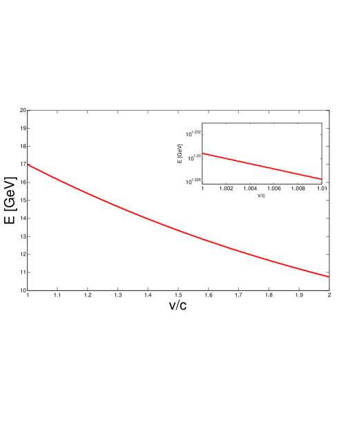
Fig. 1: $E$ in GeV as function of $v/c$ for superluminal neutrino.

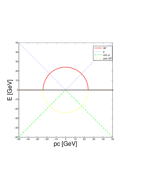
Fig. 2: $E$ in GeV as function of $pc$ in GeV: Solid line for SP, Dotted line for particle, Dashed line for antiparticle, Dashed dotted line anti-SP.

IV Application of the model to the Opera results

Applying Eq. 1 to the Opera results, the neutrino mass can be extracted

$$m_{\nu_{\mu}}c^{2}\sim{\sqrt{2}E}\sim 24.4\rm GeV\,.$$

In Fig. 1 we show $E$ in GeV versus $v/c$ where we have fixed $E=17$ GeV at $v/c=1$ for neutrino. From the inner figure of Fig. 1, we conclude that there is no significant energy-dependence of the superluminality at the vicinity of $v\sim c$. Moreover, this result can be confronted to experimental results in the future if more superluminal particles (SP) are observed with large velocity ranges. These results, can be subject to two criticisms

1. The velocity dependence like shown in Fig. 1 would lead to much larger deviations of neutrino velocity from $c$ than suggested by Opera: a large range of neutrino energies from few GeV to 80 GeV needs to be considered.

2. Also, Eq. 1 does not allow real energies for neutrino momenta above $m_{0}c^{2}$ = 24.4 GeV. This contradicts the observations from Z decay at LEP where neutrinos with energy 45.6 GeV were produced.

However, since enough experimental data for mass-matrix of the neutrinos under consideration is still absent, it is not clear its exact form for the superluminal neutrino. Here, we claim the following

“If nature allow the existence of superluminal particles they must obey to the proposed dynamics.”

In Fig. 2 we show the neutrino $E$ as function of $pc$ for particle/antiparticle and SP/anti-SP (4 branches). From Fig. 2 we expect that the neutrino becomes superluminal at the 4 points of intersection of the circle describing the Superluminal neutrino and the lines describing neutrino. We call this mechanism as the superluminality mechanism for zero mass particles.

V Application of the ELTM to Field theory

In order to show that our approach is not a simple transformation from Minkowski space to Euclidian space, which transform the action $S\rightarrow S_{E}$ , we consider the application of the model to complex local field theory. Consider as an example, a scalar field with the dispersion relation given above (Eq. 1) and defining

$$\widehat{\partial}_{\mu}=\left({\partial\over\partial t}\,,\,i{\bf\nabla}\right)\,,$$

then, the field equation can be written as ($c=\hbar=1$)

$$(\widehat{\partial}_{\mu}\widehat{\partial}^{\mu}+m^{2})\phi=0,\hskip 21.68121pt\mu=0,1,2,3$$ (2)

with $E=i\partial_{t}$ and $p=-i{\bf\nabla}$. The field equation written at this form, that is using the $\widehat{\partial}$, is used to conserve properties like covariant and contravariant. This will simplify the discussion of invariance under the following extended Lorentz transformation

$$\widehat{\Lambda}=\left(\begin{array}[]{cccc}\gamma&-\beta\gamma&0&0\\ -\beta\gamma&\gamma&0&0\\ 0&0&1&0\\ 0&0&0&1\\ \end{array}\right)=\left(\begin{array}[]{cccc}\cos\theta&i\sin\theta&0&0\\ i\sin\theta&\cos\theta&0&0\\ 0&0&1&0\\ 0&0&0&1\\ \end{array}\right)$$

where $\beta=-i{v\over c}$, and $\cos\theta=\gamma$. The invariance of Eq. 2 can be deduced from the invariance of the scalar field in standard field theory using the following transformation $\Lambda\rightarrow\widehat{\Lambda}$ and ${\partial}^{\mu}\rightarrow\widehat{\partial}^{\mu}$. Now, after studying invariance of the new scalar field, it is useful to see what happen for the dynamical quantities like Green’s function. We start from the wick-rotated functional integral of $\phi$

$$\int{\it{\mathcal{D}}}\phi(x)\exp\left[i\int d^{4}x{\mathcal{L}}(\phi)\right]$$

with ${\mathcal{L}}={1\over 2}(\widehat{\partial}_{\mu}\phi)^{2}-{1\over 2}m^{2}\phi^{2}$ is the Lagrangian density for the free scalar field. The generating function of $\phi(x)$ is

$$Z(j)=\int{\it{\mathcal{D}}}\phi(x)\exp\left[i\int d^{4}x({\mathcal{L}}(\phi)+j\phi)\right]$$

Therefore, the Green’s function integral of $\phi(x)$ can be calculated from the generating function exactly as Minkowski Green’s function that is

$$G_{F}(x,x^{\prime}) = {-1\over Z(0)}{\delta Z\over\delta j(x)\delta j(x^{\prime})}=\langle T\phi(x)\phi(x^{\prime})\rangle$$

$$= \int{d^{4}k\over(2\pi)^{4}}{e^{-ik(x-x^{\prime})}}{i\over k^{2}-m^{2}+i\epsilon}\,.$$

This Green’s function, is just the Feynman propagator with

$$k^{2}=w^{2}-{\bf k^{2}}\rightarrow k^{2}=w^{2}+{\bf k^{2}}.$$

As for the Dirac field, it is also possible to construct its wave equation. In fact, the proposed DE for SP that must be invariant under the extended Lorentz transformation is

$$(i\gamma^{\mu}\widehat{\partial}_{\mu}-m)\psi=0$$

Of course, this equation is guessed from the non superluminal particles (NSP) DE. Again, as done for scalar field, the Lorentz invariance of this equation, under the extended Lorentz group, can be deduced from the invariance of the NSP. In fact, the generators of the Lee algebra of the extended Lorentz group will be the same as Lorentz group algebra. The only change is in the antisymmetric tensor that gives the infinitesimal angle where $v/c$ must be replaced by $\beta=-iv/c$ (See any standard field theory text book). Moreover, solution of this equation can be obtained from the NSP solution of DE using the following substitution

$${\bf p}\rightarrow i{\bf p}$$ (3)

in Dirac’s spinors. Thus the positive energy solution four-spinors is

$$u^{(s)}=N\left(\begin{array}[]{c}\chi^{(s)}\\ {{\bf i\sigma p}\over m+E}\chi^{(s)}\end{array}\right)$$

and the negative energy solution is

$$u^{(s)}=N\left(\begin{array}[]{c}{{\bf-i\sigma p}\over m+|E|}\chi^{(s)}\\ \chi^{(s)}\end{array}\right)$$

where $N$ is a normalization factor and $\psi=ue^{-ipx}$. Other physical quantities for Dirac field can be obtained by the same substitution given in Eq. 3. For example when calculating cross-section for some physical process in standard model one has to take into account for SP the $m_{\nu}$ and the substitution of

$$p=(E,{\bf p})\rightarrow p=(E,i{\bf p})\,.$$

For example, the scattering cross section of superluminal $e^{+}e^{-}\rightarrow\mu^{+}\mu^{-}$ can be inferred from the subluminal scattering for the same process. In fact we found

$${\sigma}_{\rm superluminal}={\sigma}_{\rm subluminal}={4\pi\alpha^{2}\over 3s}$$

Application of this formalism to interacting fields and calculation of cross section for some physical process will be left for future investigation. In next section, as we are interested in new physics that might govern the dynamics of SP, we take this opportunity to see the smallest representation of the new DE in the newly proposed algebra 9 . This algebra is called the Generalized-$\mathbb{C}$ (G$\mathbb{C}$) extend quantum theory to new class of theories based on the non associative algebra.

VI Beyond local complex field theory description of SP

Since our aim in this paper is to search for new physics that describe SP then it is of great importance to investigate the new DE within the framework of the extended quantum mechanics that has been recently proposed in 9 . In fact, Quantum mechanics as developed in the standard textbooks, and as applied to elementary particle physics in the standard model, is understood to be complex quantum mechanics: The wave functions and probability amplitudes are represented by complex numbers. However, it has been known since the 1930s that more general quantum mechanical systems can, in principle, be constructed.

In the present work, the Generalized-$\mathbb{C}$ quantum mechanics 9 is studied for SP. However, we do not construct, a general formalism for Generalized-$\mathbb{C}$ local field theory. We only concentrate on the description of the new DE within the framework of Generalized-$\mathbb{C}$ quantum mechanics. We believe that this will be useful in future investigation of new physics. For clarity, to avoid the explicit use of $i$, the most general form of DE is

$$\mathcal{H}\psi=(C_{\mu}\partial_{\mu})\psi=(C_{x}\partial_{x}+C_{y}\partial_{y}+C_{z}\partial_{z}+C_{t}\partial_{t})\psi=m\psi.$$ (4)

To recover the new Klein-Gordon equation

$$(-\nabla^{2}-\partial_{t}^{2})\psi=m^{2}\psi,$$

the following conditions must hold

$$C_{x,y,z}^{2}=-1;\hskip 7.22743ptC_{t}^{2} = -1;\hskip 7.22743pt$$

$$\left\{C_{\mu},C_{\nu}\right\}=C_{\mu}C_{\nu}+C_{\nu}C_{\mu} = 0,$$

$$\mbox{ where }\mu\neq\nu.\hskip 7.22743pt\mu,\nu = x,y,z,t$$ (5)

Using the following Dirac matrices, satisfying (5)

$$C_{t}=\left(\begin{array}[]{cccc}0&e_{1}\\ e_{1}&0\end{array}\right)$$

$$C_{x}=\left(\begin{array}[]{cccc}0&e_{2}\\ e_{2}&0\end{array}\right)$$

$$C_{y}=\left(\begin{array}[]{cccccccc}e_{1}&0\\ 0&-e_{1}\end{array}\right)$$

$$C_{z}=\left(\begin{array}[]{cccc}e_{2}&0\\ 0&-e_{2}\end{array}\right)$$

($e_{1},e_{2}$ are the imaginary G$\mathbb{C}$ units, see Appendix), in equation(4) results in:

$$(\mathcal{H}-m)\psi=$$

$$\left(\begin{array}[]{cccc}-m+e_{1}\partial_{y}+e_{2}\partial_{z}&e_{1}\partial_{t}+e_{2}\partial_{x}\\ e_{1}\partial_{t}+e_{2}\partial_{x}&-m-e_{1}\partial_{y}-e_{2}\partial_{z}\end{array}\right)\left(\begin{array}[]{c}\psi_{1}\\ \psi_{2}\end{array}\right)=0$$ (10)

The solution to this equation in 1+1 dimension, $y,t$, is

$$\psi(y,t)=N\left(\begin{array}[]{c}{E\over p+m}\\ 1\end{array}\right)e^{e_{1}(py-Et)}\quad\,$$ (11)

where, as usual $p$ represents the ‘momentum’, $E$ is the ‘energy’ and $N$ is a normalization factor. As expected $E=\pm\sqrt{-p^{2}+m^{2}}$. Note that the importance of G$\mathbb{C}$ algebra is in the existence of complex solution in small dimension (here 2) which is not available in $\mathbb{C}$ algebra.

VII Conclusions

We have attempted to account for neutrino superluminality, as reported by OPERA, while staying within the familiar framework of local field theory. We show that superluminal neutrinos can be fitted into the original Standard Model without changing other results. Since enough experimental data for mass-matrix of the neutrinos is still absent, it is not clear what is the exact form of it. However, using the extended Lorentz transformation model we have provided an estimation of this mass. It is also found, in this paper, a two dimensional Dirac’s wave function for the new dispersion relation within the framework of the three dimensional non-associative algebra. Finally we believe that the proposed models merits to be explored in more physical problem.

Appendix

We remind the reader about the properties of the Generalized-$\mathbb{C}$ algebra (G$\mathbb{C}$). An interested reader may refer to 9 ; 10 for further information. The proposed generalization of the $\mathbb{C}$ algebra, the G$\mathbb{C}$, is finite-dimensional non division algebra containing the real numbers $\mathbb{R}$ as a sub-algebra and has the following properties:

• A general G$\mathbb{C}$ number, q, can be written as

  $$q=ae_{0}+be_{1}+ce_{2}$$

  where

  $$\emph{a,b,c}\in\mathbb{R}\,\rm or\,\mathbb{C}\,,$$

  The real $e_{0}=1$ and the imaginary G$\mathbb{C}$ units, $e_{1},e_{2}$ are defined by

  $$e_{1}e_{1}=e_{2}e_{2}=-1\,,\quad e_{1}e_{2}=e_{2}e_{1}=0$$

• The addition is defined as

  $$q_{1}+q_{2}=a_{1}+a_{2}+(b_{1}+b_{2})e_{1}+(c_{1}+c_{2})e_{2}\,,$$

  is associative

  $$q_{1}+(q_{2}+q_{3})=(q_{1}+q_{2})+q_{3}\,.$$

• The multiplication is defined as

  $$q_{1}q_{2}=a_{1}a_{2}-b_{1}b_{2}-c_{1}c_{2}+(a_{1}b_{2}+b_{1}a_{2})e_{1}+(a_{1}c_{2}+c_{1}a_{2})e_{2}\,,$$

  is non-associative under multiplication that is $(q_{1}q_{2})q_{3}\neq q_{1}(q_{2}q_{3})$.

• The norm of an element $q$ of G$\mathbb{C}$ is defined by

  $$N(q)=(\bar{q}q)^{1/2}=(a^{2}+b^{2}+c^{2})^{1/2}$$

  with the G$\mathbb{C}$ conjugate $\bar{q}$ given by

  $$\bar{q}=a-be_{1}-ce_{2}\,.$$

References

- (1) T. Adam et al. (OPERA Collaboration) (2011), 1109.4897.
- (2) P. Adamson et al. (MINOS Collaboration), Phys.Rev. D76, 072005 (2007), 0706.0437.
- (3) S. S. Gubser, Phys.Lett. B705, 279 (2011), 1109.5687.
- (4) G. Amelino-Camelia, L. Freidel, J. Kowalski-Glikman, and L. Smolin (2011), * Temporary entry *, 1110.0521.
- (5) G. Dvali and A. Vikman (2011), 1109.5685.
- (6) A. Kehagias (2011), * Temporary entry *, 1109.6312.
- (7) I. Oda and H. Taira (2011), 1110.0931.
- (8) J. Alexandre, J. Ellis, and N. E. Mavromatos (2011), 1109.6296.
- (9) B. Alles, http://arxiv.org/abs/1111.0805
- (10) L. Iorio, http://arxiv.org/abs/1109.6249
- (11) E. Saridakis, http://arxiv.org/abs/1110.0697
- (12) J. S. Diaz and V. A. Kostelecky, Phys. Lett. B 700, 25 (2011) arXiv:1012.5985 [hep-ph]
- (13) S. Hamieh etal. arXiv:1104.3416 [math-ph], accepted for publication in Journal of Modern Physics
- (14) S. Adler. Quaternion Quantum Mechanics and Quantum Fields. Oxford University Press, New York, (1995).