NONLINEAR PLASMA DIPOLE OSCILLATIONS
IN SPHEROIDAL METAL NANOPARTICLES

Abstract

The theory of nonlinear dipole plasma oscillations generated in a metal spheroidal nanoparticle by a laser-wave field has been developed. Approximate (to within the cubic term) analytic expressions for the nanoparticle dipole moment have been obtained in the case where the laser field is oriented along the spheroid rotation axis.

1 Introduction

When the center of masses of the electron subsystem in a metal nanoparticle is shifted with respect to the center of masses of the ion subsystem, there emerges an electrostatic force, which counteracts their spatial separation. This force may invoke dipole plasma oscillations in metal nanoparticles. In the first approximation, it is proportional to the relative displacement of the electron and ion centers of masses. If the displacement grows further, the electrostatic force starts to depend nonlinearly on this separation, which results in the appearance of nonlinear dipole plasma oscillations. These nonlinear plasma oscillations in metal nanoparticles were studied in works [1,​ 2,​ 3]. In works [1,​ 2], plasma oscillations were considered in the continual approximation, and the microscopic approach was taken as a basis in work [3]. In all cited works, the shape of a metal nanoparticle was assumed spherical.

Our work is devoted to the development of the theory of nonlinear plasma oscillations in metal nanoparticles of ellipsoidal shape. It should be emphasized that the results of the theory of plasma resonances in asymmetric metal nanoparticles cannot be reduced to small corrections to the results known for spherical particles, but have fundamental differences. In particular, already in the linear approximation, a spherically symmetric metal particle has one plasma resonance, whereas a spheroidal particle has two plasma resonances and an ellipsoidal particle has three ones. Therefore, the task aimed at developing the nonlinear theory of dipole plasma oscillations in asymmetric metal nanoparticles remains challenging and interesting for today.

2 Formulation of the Problem

We consider the problem of oscillations in metal nanoparticles in the continual approximation and take, as a basis, the hydrodynamic equations for the electron density $n_{e}(\mathbf{r},t)$ and the electron velocity $\bm{\upsilon}(\mathbf{r},t)$ similarly to work [2]:

$$\frac{\partial n_{e}}{\partial t}+\bm{\nabla}\;(n_{e}\bm{\upsilon})=0,$$ (1)

$$\frac{\partial\bm{\upsilon}}{\partial t}+(\bm{\upsilon}\;\bm{\nabla})\bm{\upsilon}=\frac{\mathbf{F}}{m_{e}}\equiv\frac{1}{m_{e}}\times$$

$$\times\left\{{-e\,\mathbf{E}_{L}+e\left[{\bm{\nabla}\Phi_{e}+\bm{\nabla}\,\Phi_{i}}\right]\,-\frac{\bm{\nabla}\,p}{n_{e}}}\right\}.$$ (2)

In Eq. (2), $\mathbf{F}(\mathbf{r},t)$ is the total force that acts on the electron liquid. It is composed of the action of the electric field generated by the laser wave, $\mathbf{E}_{L}$, and the action of the gradients of electron, $\Phi_{e}$, and ion, $\Phi_{i}$, potentials, and the pressure, $p$, gradient. In the dipole approximation, the field $\mathbf{E}_{L}$ is considered spatially uniform within a nanoparticle.

Let us introduce a vector that characterizes the position of the center of masses of the electron subsystem,

$$\mathbf{u}\,(t)=N_{e}^{-1}\int{d^{3}\,r\,n_{e}(\mathbf{r},t)\,\mathbf{r}},$$ (3)

where $N_{e}$ is the total number of electrons in the metal nanoparticle. With regard for Eq. (1), the equation of motion for the center of masses of the electron subsystem looks like

$$N_{e}\;\frac{d^{2}\mathbf{u}}{dt^{2}}=\int{d^{3}r\,\frac{\partial^{2}n_{e}\,(\mathbf{r},t)}{\partial t^{2}}}\;\mathbf{r}=$$

$$=\int{d^{3}r\;n_{e}(\mathbf{r},t)\;\left({\frac{\partial\bm{\upsilon}}{\partial t}+(\bm{\upsilon}\,\bm{\nabla})\,\bm{\upsilon}}\right)}.$$ (4)

Rewriting it in the form

$$m_{e}\;\mathbf{u}=N_{e}^{-1}\langle\,\mathbf{F}\,\rangle,$$ (5)

and using Eq. (2), we obtain

$$\langle\mathbf{F}\rangle=-e\;E_{L}(t)N_{e}+$$

$$+\!\!\int\!\!{d^{3}r\,\left\{{e\,\left[{\bm{\nabla}\Phi_{e}(\mathbf{r},t)+\bm{\nabla}\Phi_{i}(\mathbf{r},t)}\right]\,n_{e}(\mathbf{r},t)-\bm{\nabla}p\,(\mathbf{r},t)}\right\}}.$$ (6)

Above, we have briefly reproduced the approach to plasma dipole oscillations in metal nanoparticles used in work [2]. The authors of work [2], by making the required estimations, adopted an approximation, whose essence is the assumption that the electron subsystem of a nanoparticle shifts as a whole (without deformations) together with the center of masses of electrons. This allows us to put

$$n_{e}\,(\mathbf{r},t)=n_{e}^{(0)}\,(\,|\mathbf{r}-\mathbf{u}\,(t)|),$$

$$\Phi_{e}\,(\mathbf{r},t)=\Phi_{e}^{(0)}\,(\,|\mathbf{r}-\mathbf{u}\,(t)|),$$ (7)

$$\mathbf{p}\,(\mathbf{r},t)=p_{0}\,(\,|\mathbf{r}-\mathbf{u}\,(t)|).$$

We note that, at the thermodynamic equilibrium (i.e., in the absence of $\mathbf{E}_{L}\,(t)$), the equality

$$e\,\left[{\bm{\nabla}\Phi_{e}^{(0)}+\bm{\nabla}\Phi_{i}^{(0)}}\right]-\frac{\bm{\nabla}\,\rho^{(0)}}{n_{e}}=0$$ (8)

is valid. In this case, Eqs. (6) and (7) yield

$$\langle\mathbf{F}\,\rangle=-e\,\mathbf{E}_{L}\,(t)\,N_{e}+\int{d^{3}r\,e\,\bm{\nabla}\,\Phi_{i}^{(0)}(\mathbf{r})}n_{e}^{(0)}(|\mathbf{r}-\mathbf{u}(t)|)=$$

$$=-e\,\mathbf{E}_{L}(t)\;N_{e}+\frac{\partial}{\partial\mathbf{u}}\,\int{d^{3}\,r\,e\,\Phi_{i}^{(0)}(\mathbf{r})\;n_{e}^{(0)}(|\mathbf{r}-\mathbf{u}|)}.$$ (9)

We use this formula as the basic one.

In contrast to the previous works [1,​ 2,​ 3] where plasma nonlinear oscillations in spherically symmetric metal nanoparticles were considered, we analyze asymmetric nanoparticles. Let a metal nanoparticle have the shape of an ellipsoid of revolution (spheroid). Let the coordinate $0Z$ axis be oriented along the spheroid symmetry axis. In addition, we suppose that the laser field $\mathbf{E}_{L}(t)$, as well as a shift of the center of masses of the electron subsystem induced by the field, is directed along the $0Z$ axis. To emphasize this fact, we use the notation

$$\mathbf{u}\equiv\mathbf{z}_{0}$$ (10)

in what follows. It is worth noting that, if the particle’s shape differs from the sphere, and the laser field that generates plasma oscillations is not oriented strictly along the symmetry axis, the various plasma resonances are coupled with one another in the nonlinear approximation, and the problem becomes incredibly complicated. Our calculations given below show that even the simplest model presented above and allowing for deviations from spherical symmetry is already capable to produce qualitatively new results, as compared with the spherical case.

Up to now, except for formulas (7) and (9), the nanoparticle symmetry has not been specified. Similarly to work [2], we adopt that the electron subsystem shifts as a whole (without deformations) together with its center of masses. Hence, we adopt that

$$n_{e}(\mathbf{r},t)=n_{0}\,\Delta_{0}\,(R(\theta)-|\,\mathbf{r}-\mathbf{z}_{0}|),$$ (11)

where $n_{0}$ is the concentration of electrons, and $\Delta_{0}(x)$ is the step-like function

$$\Delta_{0}(x)={\left\{{\begin{array}[]{l}1,\quad x>0,\\ 0,\quad x<0.\\ \end{array}}\right.}$$ (12)

The function $R(\theta)$ defines the spheroid surface (to be more specific, let the spheroid be prolate),

$$R\,(\theta)=\frac{R_{\bot}}{\sqrt{1-e_{p}^{2}\,\cos^{2}\theta}},$$ (13)

where $e_{p}$ is the spheroid eccentricity,

$$e_{p}^{2}=\;\left|{\,\frac{R_{\perp}^{2}}{R_{\parallel}^{2}}\;-1\;}\right|,$$ (14)

$\theta$ is the angle between the axis $0Z$ and the $\mathbf{R}(\theta)$ on the spheroid surface, and $R_{||}$ and $R_{\bot}$ are the longitudinal (along the symmetry axis) and transverse, respectively, curvature radii.

Supposing, in analogy with Eq. (7), that the structures of functions $\Phi_{e}(\mathbf{r},t)$ and $p\,(\mathbf{r},t)$ are similar to that of the function $n_{e}(\mathbf{r},t)$ given by formula (11), we obtain

$$\langle\mathbf{F}\rangle=-e\,\mathbf{E}_{L}(\,t\,)\;N_{e}+n_{0}\times$$

$$\times\int{d^{3}r\;e\;\bar{\nabla}\;\Phi_{i}^{(0)}(\,\mathbf{r}\,)\;\Delta_{0}\;(R(\theta)-|\,\mathbf{r}-\mathbf{z}_{0}\,|)}$$ (15)

instead of formula (9). Hence, in order to determine the force $\left\langle\mathbf{F}\right\rangle$ that counteracts a displacement of the electron subsystem in a spheroidal metal nanoparticle along the axis $0Z$, we have to determine the ionic electrostatic potential $\Phi_{i}^{(0)}$. This will be done in the next section.

3 Electrostatic Potential of a Charged Spheroid

The electrostatic potential generated by the ion core in a spheroidal nanoparticle looks like

$$\Phi_{i}^{(0)}=\int\limits_{V}{\frac{\rho_{i}\,d^{3}r}{|\;\mathbf{r}-{\mathbf{r}}^{\prime}\;|}}.$$ (16)

Let the density of ion charges be uniformly distributed over the volume $V$,

$$\rho_{i}={e\,N_{i}\,Z_{i\;}}/V={\mathrm{const}},$$ (17)

where $N_{i}$ is the number of ions, and $Z_{i}$ is the charge multiplicity. Taking the spheroid symmetry and the charge uniformity into account, Eq. (16) takes the form

$$\Phi_{i}^{(0)}=\rho_{i}\int\limits_{0}^{2\pi}{d\,{\varphi}^{\prime}\int\limits_{0}^{\pi}{d\,{\theta}^{\prime}\,\sin\,{\theta}^{\prime}}}\int\limits_{0}^{R\,({\theta}^{\prime})}{\frac{d{r}^{\prime}\,{r}^{\prime}{}^{2}}{|\mathbf{r}-{\mathbf{r}}^{\prime}|}}.$$ (18)

To carry out the integration in Eq. (18), it is expedient to make the expansion

$$\frac{1}{|\,\mathbf{r}-{\mathbf{r}}^{\prime}\,|}=\sum\limits_{n=0}^{\infty}{{P}_{n}\,(\cos\nu)}\left\{{\begin{array}[c]{l}\frac{1}{r}\left({\frac{{r}^{\prime}}{r}}\right)^{n}\quad\mathrm{at}\quad{r}^{\prime}<r,\\ \frac{1}{{r}^{\prime}}\left({\frac{r}{{r}^{\prime}}}\right)^{n}\quad\mathrm{at}\quad{r}^{\prime}>r,\\ \end{array}}\right.$$ (19)

where $\nu$ is the angle between the vectors $\,\mathbf{r}$ and ${\mathbf{r}}^{\prime}$, and apply the relation [4]

$${P}_{n}\,(\cos\,\nu)={P}_{n}\,(\cos{\theta}^{\prime})\;{P}_{n\,}(\cos\theta)+$$

$$+2\sum\limits_{m}{\frac{(n-m)!}{(n+m)!}\cos({\varphi}^{\prime}-\varphi)\,{P}_{n}^{m}\,(\cos{\theta}^{\prime})}\,{P}_{n}^{m}(\cos\theta).$$ (20)

The angles $({\varphi}^{\prime},{\theta}^{\prime})$ and $(\varphi,\theta)$ in Eq. (20) describe the spatial orientations of the vectors $\mathbf{r}^{\prime}$ and ${\mathbf{r}}$, respectively. When substituting Eq. (20) in Eq. (18) and integrating the result obtained over ${\varphi}^{\prime}$, the second term in Eq. (20) is nulled.

According to Eq. (13), the quantity $R({\theta}^{\prime})$ in Eq. (18) satisfies the condition

$$R_{\perp}\leq R\,({\theta}^{\prime})\leq R_{\parallel}.$$ (21)

Therefore, it is expedient to consider the integral over $\mathbf{r}^{\prime}$ in three cases:

$$a)\leavevmode\nobreak\ r\,\leq\,R_{\perp},$$

$$b)\leavevmode\nobreak\ R_{\perp}\leq r\,\leq\,R_{\parallel},\leavevmode\nobreak\ \leavevmode\nobreak\ \mathrm{and}$$

$$c)\leavevmode\nobreak\ R_{\parallel}\,\,\leq\,\,r.$$ (22)

At $r\,\leq\,R_{\perp}$, in accordance with Eqs. (18)–(20), we obtain

$$\Phi_{i}^{(0)}=2\pi\,\rho_{i}\sum\limits_{n=0}^{\infty}{P_{n}\,(\cos\theta)\int\limits_{0}^{\pi}{d{\theta}^{\prime}\,\sin{\theta}^{\prime}{P}_{n}\,(\cos{\theta}^{\prime})}}\times$$

$$\times\left\{{\frac{1}{r}\int\limits_{0}^{r}{d{r}^{\prime}\;{r}^{\prime}{}^{2}\left({\frac{{r}^{\prime}}{r}}\right)^{n}+\int\limits_{r}^{R({\theta}^{\prime})}{d{r}^{\prime}\;{r}^{\prime}\;\left({\frac{r}{{r}^{\prime}}}\right)^{n}}}}\right\}.$$ (23)

The further calculation of the integrals in formula (23) has no difficulties. A more difficult situation arises in the case $R_{\bot}\leq r\leq R_{\|}$, because, in accordance with Eq. (21), the variable $r^{\prime}$ changes in the same interval. Therefore, depending on the angle $\theta^{\prime}$, the maximum value of $r^{\prime}$ can be both larger and smaller than $r$ (see Fig. 1). It is expedient to introduce an angle $\theta_{1}$, at which the ellipsoid and the sphere of radius $r$ intersect; in other words,

$$R\,({\theta}^{\prime})=R\,(\theta_{1})=r.$$ (24)

In view of Eq. (13), Eq. (24) yields

$$\cos\theta_{1}=\frac{1}{e_{\rho}}\left\{{1-\left({\frac{R_{\bot}}{r}^{2}}\right)}\right\}^{1/2}.$$ (25)

Now, let us decompose the integral over $\theta^{\prime}$ in Eq. (18) as follows:

$$\int\limits_{0}^{\pi}{d{\theta}^{\prime}}\ldots=\int\limits_{0}^{\theta_{1}}{d{\theta}^{\prime}\ldots+\int\limits_{\theta_{1}}^{\pi-\theta_{1}}{d{\theta}^{\prime}}}\ldots+\int\limits_{\pi-{\theta}_{1}}^{\pi}{d{\theta}^{\prime}\ldots}\leavevmode\nobreak\ .$$ (26)

Figure 1 demonstrates that $r^{\prime}$ can be both larger and smaller than $r$ in the intervals $0<\theta^{\prime}<\theta_{1}$ and $\pi-\theta_{1}<\theta^{\prime}<\pi$. At the same time, $r^{\prime}$ is always smaller than $r$ in the interval $\theta_{1}<\theta^{\prime}<\pi-\theta_{1}$. Substituting expansion (19) in Eq. (18) and dividing the integration interval in accordance with procedure (26), we obtain

$$\Phi_{i}^{(0)}=2\pi\rho_{i}\sum\limits_{n=0}^{\infty}{P_{n}(\cos\theta)}\Biggl{\{}\int\limits_{0}^{\theta_{1}}{d{\theta}^{\prime}\sin{\theta}^{\prime}{P}_{n}(\cos{\theta}^{\prime})}\times$$

$$\times\Bigg{[}\frac{1}{r}\int\limits_{0}^{r}{d{r}^{\prime}{r}^{\prime 2}\left({\frac{{r}^{\prime}}{r}}\right)^{n}}+\int\limits_{r}^{R({\theta}^{\prime})}{d{r}^{\prime}{r}^{\prime}\left({\frac{r}{{r}^{\prime}}}\right)^{n}}\Bigg{]}+$$

$$+\int\limits_{\theta_{1}}^{\pi-\theta_{1}}{d{\theta}^{\prime}\sin{\theta}^{\prime}P_{n}(\cos{\theta}^{\prime})\frac{1}{r}}\int\limits_{0}^{R({\theta}^{\prime})}{d{r}^{\prime}{r}^{\prime 2}\left({\frac{{r}^{\prime}}{r}}\right)^{n}+}$$

$$+\int\limits_{\pi-{\theta}_{1}}^{\pi}{d{\theta}^{\prime}\sin{\theta}^{\prime}{P}_{n}(\cos{\theta}^{\prime})}\times$$

$$\times\Bigg{[}\frac{1}{r}\,\int\limits_{0}^{r}{d{r}^{\prime}{r}^{\prime 2}\left({\frac{{r}^{\prime}}{r}}\right)^{n}}+\int\limits_{r}^{R({\theta}^{\prime})}{d{r}^{\prime}{r}^{\prime}\left({\frac{r}{{r}^{\prime}}}\right)^{n}}\Bigg{]}\Biggr{\}}.$$ (27)

Making substitutions of the type ${\theta}^{\prime}\div\pi-{\theta}^{\prime}$ in the last term of Eq. (27), the whole expression (27) can be expressed in the form

$$\Phi_{i}^{(0)}=2\pi\rho_{i}\sum\limits_{n=0}^{\infty}{P_{n}\,(\cos\theta)}\Bigg{\{}\int\limits_{0}^{\theta_{1}}{d{\theta}^{\prime}\,\sin{\theta}^{\prime}}\times$$

$$\times\left[{P}_{n}(\cos{\theta}^{\prime})+{P}_{n}(-\cos{\theta}^{\prime})\right]\times$$

$$\times\Bigg{[}\frac{1}{r}\int\limits_{0}^{r}{d{r}^{\prime}\,{r}^{\prime}{}^{2}\left({\frac{{r}^{\prime}}{r}}\right)^{n}}+\int\limits_{r}^{R({\theta}^{\prime})}{d{r}^{\prime}\,{r}^{\prime}\left({\frac{r}{{r}^{\prime}}}\right)^{n}}\Bigg{]}+$$

$$+\int\limits_{\theta_{1}}^{\pi/2_{1}}{d{\theta}^{\prime}\sin{\theta}^{\prime}}\left[P_{n}(\cos{\theta}^{\prime})+{P}_{n}(-\cos{\theta}^{\prime})\right]\times$$

$$\times\frac{1}{r}\int\limits_{0}^{R({\theta}^{\prime})}{d{r}^{\prime}{r}^{{\prime}^{2}}\left(\frac{{r}^{\prime}}{r}\right)^{n}}\Bigg{\}}.$$ (28)

One can see that all terms with odd powers of $n$ disappear from sum (28). Expression (28) describes $\Phi_{i}^{(0)}$ in the range $R_{\perp}\leq r\leq R_{\parallel}$.

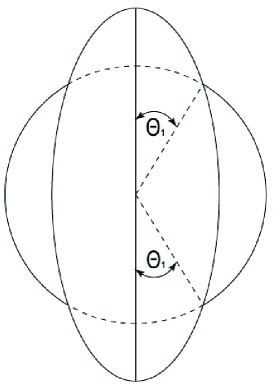
Fig. 1:

At last, let us consider the case $r\geq R_{\parallel}$, where $r^{\prime}<r$. From Eqs. (18) and (19), we obtain

$$\Phi_{i}^{(0)}=2\pi,\rho_{i}\sum\limits_{n=0}^{\infty}P_{n}\,(\cos\theta)\int\limits_{0}^{\pi}{d{\theta}^{\prime}\,\sin{\theta}^{\prime}\times{P}_{n}(\cos{\theta}^{\prime})}\times$$

$$\times\frac{1}{r}\int\limits_{0}^{R({\theta}^{\prime})}{d{r}^{\prime}\,{r}^{\prime 2\;}\left({\frac{{r}^{\prime}}{r}}\right)}^{n}.$$ (29)

As is seen from expressions (23), (28), and (29), we can write

$$\Phi_{i}^{(0)}=\sum\limits_{n=0}^{\infty}{{P}_{n}(\cos\theta)\Psi(n)=\Psi(0)+}$$

$${+{P}_{2}(\cos\theta)\Psi(\ref{eq2})+{P}_{4}(\cos\theta)\Psi(\ref{eq4})+\cdots}$$ (30)

for the whole range of variation of the vector $\mathbf{r}$. Integrating in Eqs. (23), (28), and (29), we obtain the expressions for the coefficients $\Psi(n)$. In particular, at $r\leq R_{\perp}$, we find

$$\Psi(0)=2\pi\rho_{i}\left\{{-\frac{r^{2}}{3}+\frac{R_{\perp}^{2}}{2e_{p}}\ln\left({\frac{1+e_{p}}{1-e_{p}}}\right)}\right\};\leavevmode\nobreak\ \leavevmode\nobreak\ r\leq R_{\bot},$$ (31)

using Eq. (23). From Eq. (28), we obtain that, at $R_{\bot}\leq r\leq R_{\parallel}$,

$$\Psi(0)=2\,\pi\rho_{i}\biggl{\{}\frac{r^{2}}{3}(\cos\theta_{1}-1)-$$

$$-\frac{R_{\perp}^{2}}{2e_{p}}\ln\,\left({\frac{1+e_{p}\cos\theta_{1}}{1-e_{p}\cos\theta_{1}}\;\frac{1-e_{p}}{1+e_{p}}}\right)+\frac{2R_{\perp}^{2}}{3}\cos\theta_{1}\biggr{\}},$$

$$R_{\perp}\leq r\leq R_{\parallel}.$$ (32)

At last, Eq. (29) implies that, at $r\geq R_{\parallel}$,

$$\Psi(0)=\frac{4}{3}\pi\rho_{i}R_{\perp}^{2}{R_{\parallel}}R_{\parallel}/r,\quad r\geq R_{\parallel}$$ (33)

Similar expressions for $\Psi(2)$ are given in Appendix.

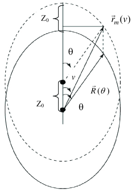
Fig. 2:

As is seen from Eq. (25), $\cos\theta_{1}=0$ at $r=R_{\bot}.$ Therefore, Eq. (32) coincides with Eq. (31). At $r=R_{\|}$, we have $\cos\theta_{1}=1$, and expression (32) coincides with (33).

Passing from the ellipsoidal shape to the limiting case of the spherical shape ($R_{\bot}=\,R_{\parallel}\equiv R$), i.e. at $e_{p}\rightarrow 0$, it is easy to see that $\Psi(n)\rightarrow 0$ for all $n\neq 0$. Concerning $\Psi(0)$, Eqs. (31)–(33) show that, at this limiting transition,

$$\Psi(0)\rightarrow\Psi^{(s)}=V\,\rho_{i}\;\left\{{\begin{array}[c]{l l}{\left({3-\frac{r^{2}}{R^{2}}}\right)}/{2R,}&{\mathrm{at}\quad r<R}\\ \frac{1}{r},&\mathrm{at}\quad r>R\\ \end{array}}\right\},$$ (34)

where $V=\frac{4\pi}{3}R^{3}$ is the sphere volume. Expression for $\Psi^{(s)}$ in the form (34) was used in [2], while considering nonlinear plasma oscillations in a spherical metal nanoparticle.

4 Electrostatic Force

Provided that the field $\mathbf{E}_{L}(t)$ is oriented along the axis $0Z,$ and the particle shape has the adopted symmetry, the field $\langle F\rangle$ is also directed along the axis $0Z$, i.e.,

$$\langle F\rangle=-eE_{L}(t)\,N_{e}+$$

$$+n_{0}\,e\,\int{d^{3}r\,\mathbf{K}_{0}\,\bm{\nabla}}\;\Phi_{i}^{(0)}(\mathbf{r})\,\Delta_{0}\,\left({R(\theta)-\left|{\,\mathbf{r}-\mathbf{z}_{0}\,}\right|\,}\right),$$ (35)

where $\mathbf{K}_{0}$ is a unit vector directed along the axis $0Z$. The integration range over $\mathbf{r}$ in Eq. (35) is defined by the condition that the argument in the step-like function $\Delta_{0}$ is larger than or equal to zero, i.e.,

$$R(\theta)-\left|{\,\mathbf{r}-\mathbf{z}_{0}}\right|\geq 0.$$ (36)

In the case where relation (36) is the equality, we obtain a root

$$r\equiv r_{m}(\nu)=\left\{{\,R^{2}(\theta)-z_{0}^{2}\;\sin^{2}\nu\,}\right\}^{1\mathord{\left/{\vphantom{12}}\right.\kern-1.2pt}2}+z_{0}\,\cos\nu.$$ (37)

As is seen from Fig. 2, the vector $\mathbf{r}_{m}(\nu)$ corresponds to that point on the surface of a shifted spheroid, which is determined by the vector $\mathbf{R}(\theta)$ on the surface of the initial spheroid. At the shift, the vector $\mathbf{R}(\theta)$ moves in parallel to itself from point 0 to point $0^{\prime}$. According to Fig. 2, we can write

$$\mathbf{r}_{m}(\nu)\,\cos\nu=z_{0}+R(\theta)\,\cos\theta,$$ (38)

$$\mathbf{r}_{m}(\nu)\,\sin\nu=R(\theta)\,\sin\theta.$$ (39)

Multiplying relations (38) and (39) by $\sin\nu$ and $\cos\nu$, respectively, and subtracting the results, we obtain

$$z_{0}\,\sin\nu=R(\theta)\;\sin(\theta-\nu).$$ (40)

This formula gives a relation between the angles $\theta$ and $\nu$ at a fixed $z_{0}$. At $z_{0}\rightarrow 0$, we obtain $\theta\rightarrow\nu$. Since the ratio $z_{0}/R(\nu)$ is small, we can write

$$\theta=\nu+\Delta\,\nu$$ (41)

so that $\Delta\nu$ can be determined from Eq. (40) by iterations:

$$\Delta\nu_{1}=\frac{z_{0}}{R(\nu)}\sin\nu;$$

$$\Delta\,\nu_{2}=\frac{z_{0}}{R(\nu)}\sin\nu\left({1-\frac{{R}^{\prime}(\nu)}{R(\nu)}\Delta\nu_{1}}\right);$$

$$\Delta\,\nu_{3}=\frac{z_{0}}{R(\nu)}\sin\nu\left({1-\frac{{R}^{\prime}(\nu)}{R(\nu)}\Delta\nu_{2}}\right),\ldots\leavevmode\nobreak\ .$$ (42)

To obtain the explicit dependence of $\mathbf{r}_{m}(\nu)$ on the shift $z_{0}$, let us expand Eq. (37) in a series (the function $R(\theta)$ should also be expanded with the use of relations (41) and (42))

$$r_{m}(\nu)=R(\nu)+z_{0}(1-e_{p}^{2})\frac{\cos\nu}{1-e_{p}^{2}\cos^{2}\nu}-$$

$$-z_{0}^{2}\;\frac{1-e_{p}^{2}}{2R_{\perp}}\frac{\sin^{2}\nu}{(1-e_{p}^{2}\cos^{2}\nu)^{3/2}}+$$

$$+z_{0}^{3}\,\frac{e_{p}^{2}}{2R_{\bot}^{2}}\left({\frac{1}{3}+\frac{1-e_{p}^{2}}{(1-e_{p}^{2}\,\cos^{2}\nu)^{2}}}\right)\,\cos\nu\,\sin^{4}\nu\,+\ldots\leavevmode\nobreak\ .$$ (43)

For the spherical shape ($e_{p}\rightarrow 0$), Eq. (37) yields

$$\mathbf{r}_{m}(\nu)=R+z_{0}\cos\nu-\frac{z_{0}^{2}}{2R}\sin^{2}\nu-\frac{z_{0}^{4}}{8R^{3}}\sin^{4}\nu+\ldots\leavevmode\nobreak\ .$$ (44)

Comparing expressions (43) and (44), we see that, in the case of an asymmetric particle ($e_{p}\neq 0$), an extra cubic nonlinearity absent in expression (44) emerges.

To avoid a misunderstanding, we should emphasize that, in what follows, the term “asymmetric particle”, will mean a particle, whose shape differs from the spherical one, rather than the absence of any symmetry elements.

Note that formula (35) with regard for Eqs. (36) and (37) can be written in the form

$$\langle F\rangle=-eE_{L}(t)\,N_{e}+$$

$$+2\pi\,n_{0}\,e\,\int\limits_{0}^{\pi}{d\nu\sin\nu}\int\limits_{0}^{r_{m}(\nu)}{dr\,r^{2}}\left[{\mathbf{K}_{0}\,\bm{\nabla}\,\Phi_{i}^{(0)}(r)}\right].$$ (45)

Expressing $r_{m}(\nu)$ as

$$\mathbf{r}_{m}(\nu)=R(\nu)+\Delta r(\nu),$$ (46)

and comparing it with Eq. (43), we see that only $\Delta r(\nu)$ depends on the shift $z_{0}$, and $\Delta r\ll R(\nu)$. It would seem that the integral over $r$ in Eq. (45) can be expanded in a power series in powers of $\Delta r_{m}(\nu)$ to obtain terms, both linear and nonlinear in $z_{0}$. However, there is a subtle point. In order to obtain terms nonlinear in $z_{0}$, we must differentiate the integrand in Eq. (45), i.e. the function

$$w(r)=r^{2}\left[{\mathbf{K}_{0}\bm{\nabla}\,\Phi_{i}^{(0)}}\right].$$ (47)

However, as is seen, e.g., from the exact expression for the ion electrostatic potential in the spherical case (34), the function $\Psi^{(s)}(r)$ and its first derivative are continuous at the point $r=R$, i.e. across the particle surface. But already the second derivative of $\Psi^{(s)}(r)$ is discontinuous at this point. Therefore, the mentioned integral cannot be expanded in a Taylor series at the surface. At the same time, the ion electrostatic potential is described by smooth functions to the left and to the right from the surface. Therefore, we will do as follows. Let us divide the integration path over $\nu$ in Eq. (45) into intervals, in which $r_{m}(\nu)$ lies only to the left or only to the right from the nanoparticle surface. Then, to the left and to the right from the surface, there exist the eligible reasons for function (47) to be expanded into a Taylor series.

Let us explain the essence of our approach using, as an example, the spherical shape, for which the results are already known [1,​ 2]. Hence, the integral entering Eq. (45) can be rewritten as follows:

$$\int\limits_{0}^{\pi}{dv\,\sin v\int\limits_{0}^{r_{m}(v)}{dr\,r^{2}\left[{\mathbf{K}_{0}\bm{\nabla}\Phi_{i}^{(0)}}\right]}}=$$

$$=\int\limits_{0}^{\pi/2}{dv\,\sin v\int\limits_{0}^{r_{m}(v)}{dr\,w(r)+\int\limits_{\pi/2}^{\pi}{dv\,\sin v\int\limits_{0}^{r_{m}(v)}{dr\,w(r)}}}}.$$ (48)

As is seen from Eq. (44), $r_{m}(\nu)\geq R$ for the first integral, and $r_{m}(\nu)\leq R$ for the second one (these inequalities become somewhat violated at $v\approx\pi/2$, but this does not make an appreciable contribution to the integral). In the case of the spherical shape in accordance with Eqs. (34) and (37), we have

$$w(r)=-\rho_{i}\,V\,\cos\nu,\quad\mathrm{at}\leavevmode\nobreak\ \leavevmode\nobreak\ r\geq R,$$ (49)

$$w(r)=-\rho_{i}\,V\,\cos\nu\left({\frac{r}{R}}\right)^{3},\quad\mathrm{at}\leavevmode\nobreak\ \leavevmode\nobreak\ r\leq R.$$ (50)

Now, let us substitute functions (49) and (50) into the first and the second integral, respectively, on the right-hand side of expression (47). Then, let us take into consideration that $\mathbf{r}_{m}(\nu)=R+\Delta r(\nu)$, with $\Delta r(\nu)\ll R$, and make the expansion

$$\int\limits_{0}^{r_{m}(\nu)}{dr\,r^{2}}\;\left[{\mathbf{K}_{0}\,\mathbf{\nabla}\,\Phi_{i}^{(0)}(r)}\right]=$$

$$\!\!=\!\!\int\limits_{0}^{R+\Delta r(v)}\!\!\!{dr\,w(r)=\!\int\limits_{0}^{R}{dr\,w(r)\!\!+w(r)\!\Delta r}}\!+\!\frac{1}{2}\left({\frac{dw}{dr}}\right)_{R}\!(\Delta r)^{2}+$$

$$+\frac{1}{6}\left({\frac{d^{2}w}{dr^{2}}}\right)_{R}(\Delta r)^{3}+\frac{1}{24}\left({\frac{d^{3}w}{dr^{3}}}\right)_{R}(\Delta r)^{4}+\ldots\leavevmode\nobreak\ .$$ (51)

To avoid the misunderstanding, we note once again that the derivatives in Eq. (51) are not calculated at the surface ($r=R$), but at a point $r$, provided that $r$ approaches the surface from the left or from the right. In particular, in the given specific case, the matter concerns the expansion of function (50), provided that $r\rightarrow R$ and $r\leq R$.

From expressions (43) and (44), we see that $\Delta r$ is a power series in $z_{0}$, i.e.

$$\Delta r=\Delta r_{1}+\Delta r_{2}+\Delta r_{3}+\Delta r_{4},$$ (52)

where $\Delta r_{i}\sim z_{0}^{i}$. In particular, in the case of spherical symmetry, according to Eq. (44), we have

$$\Delta r_{1}=z_{0}\cos v,\quad\Delta r_{2}=-\frac{z_{0}^{2}}{2R}\sin^{2}v,$$

$$\Delta r_{3}=0,\quad\Delta r_{4}=-\frac{z_{0}^{4}}{8R^{3}}\sin^{4}v.$$ (53)

Taking into account Eqs. (51) and (52), all integrals in expression (45) can be calculated to the end, and we obtain (at $z_{0}\geq 0$)

$$\langle F\rangle=-e\,E_{L}(t)\,N_{e}-m_{e}\,N_{e}\omega_{p}^{2}\left\{{z_{0}-\frac{9}{16}\,\frac{z_{0}^{2}}{R}+\frac{z_{0}^{4}}{32R^{3}}}\right\},$$ (54)

where $\omega_{p}^{2}=\frac{4\pi\,e^{2}n_{0}}{3\,m_{e}}$ is the square of the plasma (dipole) frequency.

Thus, we repeated the result of works [1,​ 2]. Now, let us apply the same approach to the case of a spheroidal nanoparticle.

5 Nonlinear Dipole Plasma Oscillations of Asymmetric Metal Nanoparticle

In the case of a spheroidal nanoparticle with regard for Eq. (30), we have

$$\mathbf{K}_{0}\bm{\nabla}\Phi_{i}^{(0)}=\cos v\frac{\partial\Phi_{i}^{(0)}}{\partial r}-\frac{\sin v}{r}\,\frac{\partial\Phi_{i}^{(0)}}{\partial v}=$$

$$=\cos v\biggl{\{}\frac{\partial\Psi(0)}{\partial r}+\frac{\partial\Psi(2)}{\partial r}P_{2}(\cos v)+$$

$$+\frac{2}{r}\Psi(2)\left[1-P_{2}(\cos v)\right]+\ldots\biggr{\}}.$$ (55)

Below, we take into account explicitly only $\Psi(0)$, although the required calculations were also carried out making allowance for the contribution of the function $\Psi(2)$, the expression for which is presented in Appendix. Our estimates showed that the account of the contribution made by $\Psi(2)$ does correct, to some extent, the coefficients at the powers of $z_{0}$, but does not change our main conclusions.

Hence, in accordance with Eq. (43), we have

$$r_{m}(0)=R_{\parallel}+z_{0}>R_{\perp};\quad r_{m}(\pi)=R_{\parallel}-z_{0}<R_{\parallel}.$$ (56)

Taking these inequalities into account, let us split the integral over the angle $\nu$ again as was done in Eq. (48). We now substitute function (33) in the first integral on the right-hand side of Eq. (48); here, in accordance with Eq. 56, $r_{m}(0)>R_{\parallel}.$ Then, according to Eqs. (47) and (30), we have

$$w(r)=\cos v\,\,r^{2}\frac{\partial\Psi(0)}{\partial r}=-\frac{4\pi}{3}\,\rho_{i\,}R_{\perp}^{2}\;R_{\parallel}\cos v.$$ (57)

In the second integral in Eq. (48), for which $r_{m}(\pi)<R_{\parallel}$, we also suppose that $r_{m}(v)>R_{\perp}$ and use function (32). In this case, we obtain

$$w(r)=\frac{4\pi}{3}\,\rho_{i\,}\left\{{\frac{1}{e_{p}}(r^{2}-R_{\bot}^{2})^{3/2}-r^{3}}\right\}\cos v.$$ (58)

Note that the assumption $r_{m}(v)>R_{\perp}$ also means that

$$r(\pi)=R_{\parallel}-z_{0}>R_{\perp}\leavevmode\nobreak\ \leavevmode\nobreak\ \text{or}\leavevmode\nobreak\ \leavevmode\nobreak\ z_{0}<R_{\parallel}-R_{\perp}.$$ (59)

Without assumption (59), the expressions for the ion electrostatic potential, as well as the integration limits (44), are transformed into the corresponding result for a spherical particle at $e_{p}\rightarrow 0$. Condition (59) makes this passage to the limit impossible, because, if $e_{p}\rightarrow 0$, inequality (59) becomes invalid at any small, but finite value of $z_{0}$. In this case, for the passage to the limit $e_{p}\rightarrow 0$ to be eligible, one should engage function (31) rather than function (32). Hence, the substitution of Eqs. (57) and (58) in Eq. (48) gives

$$\int\limits_{0}^{\pi}{dv\sin v}\int\limits_{0}^{r_{m}(v)}{dr\left[{\mathbf{K}_{0}\bm{\nabla}\Phi_{i}^{(0)}}\right]}=$$

$$={{-\frac{4\pi}{3}R_{\perp}^{2}\,R_{\parallel}\rho_{i}\,\int\limits_{0}^{\pi/2}{dv\,r_{m}(v)\,\sin v\,\cos v\;+}}}$$

$$+\frac{4\pi}{3}\rho_{i}\!\!\int\limits_{\pi/2}^{\pi}\!\!{dv\sin v\cos v}\!\!\!{\int\limits_{0}^{r_{m}(v)}\!\!\!{dr\left\{\!{\frac{1}{e_{p}}(r^{2}\!-R_{\bot}^{2})^{3/2}-r^{3}}\!\right\}}}.$$ (60)

To integrate the second integral over $r$ in Eq. (60), we take advantage, similarly to Eq. (51), of the smallness of quantity $\Delta r$ and expand this integral in a series in $\Delta r$. However, there exists a certain difference between cases (51) and (60). In case (51), $r_{m}(v)=R+\Delta r(v),$ and in case (60), $r_{m}(v)=R(v)+\Delta r(v)$ in accordance with Eq. (43). To avoid excess complications, we expand the integral $\int_{0}^{r_{m}(v)}{dr\,\left\{\ldots\right\}}$ into a series in $\Delta r$ at the point $R_{\parallel},$ rather than at $R(v)$. A reason for this approximation is that, first, the electrostatic potential is mainly governed by the distribution of charges near the ellipsoid vertex (pole), i.e. by the range of angles, in which $R(v)\approx R_{\parallel}$, and, second, the function $\Psi(0)$ and its derivative, as is seen from Eqs. (32) and (33), are continuous at the point $r=R_{\parallel}$, similarly to what takes place in the spherical case, for which the exact solution is known.

From Eq. (60), confining the expansion to terms cubic in $\Delta r$, we obtain

$$\int\limits_{0}^{\pi}{dv\,\sin v}\int\limits_{0}^{r_{m}(v)}{dr\,r^{2}\left[{\mathbf{K}_{0}\bm{\nabla}\Phi_{i}^{(0)}}\right]}=$$

$$={{-V\,\rho_{i}\int\limits_{0}^{\pi/2}{dv\,\Delta r(v)\sin v\cos v}}}-$$

$$-V\rho_{i}\int\limits_{\pi/2}^{\pi}{dv\,\sin v\,\cos v\,\left\{{\Delta r(v)-\frac{(\Delta r(v))^{3}}{2e_{p}^{2}\,R_{\parallel}^{2}}}\right\}},$$ (61)

where $V=\frac{4\pi}{3}R_{\perp}^{2}R_{\parallel}$ is the volume of spheroid.

Note that, owing to inequality (59), the following inequality, as can be easily verified, is also valid:

$$e_{p}\,R_{\parallel}>z_{0}.$$ (62)

If inequality (62) is obeyed, the term cubic in $\Delta r$ is much smaller than the linear one, as it must be when expanding in a small parameter. Since the expression for $\Delta r(v)$ itself is a series expansion in $z_{0}$, we confine the consideration below to the terms, the order of which is not higher than $z_{0}^{3}$, i.e. we make the substitution

$$\Delta r(v)\approx\Delta r_{1}(v)+\Delta r_{2}(v)+\Delta r_{3}(v),$$

$$\left({\Delta r(v)}\right)^{3}\approx\left({\Delta r_{1}(v)}\right)^{3}$$ (63)

into Eq. (61). The form of $\Delta r_{i}(v)$-terms for the spheroidal shape is clear from expression (43).

Calculating the corresponding integrals in Eq. (61) and substituting the obtained expression into Eq. (45), we obtain

$$\left\langle F\right\rangle=-e\,E_{L}(t)\,N_{e}-m_{e}N_{e}\,\omega_{\parallel}^{2}\,z_{0}-m_{e}\,N_{e}\,\omega_{pL}^{2}\,\frac{\delta(e_{p})}{R_{\parallel}^{2}}z_{0}^{3},$$ (64)

where

$$\omega_{\parallel}^{2}=L_{\parallel}\omega_{pL}^{2}\equiv\frac{1-e_{p}^{2}}{2e_{p}^{3}}\left\{{\ln\left({\frac{1+e_{p}}{1-e_{p}}}\right)-2e_{p}}\right\}\omega_{pL}^{2},$$ (65)

$\omega_{pL}=\sqrt{{\frac{4\pi n_{0}e^{2}}{m_{e}}}}$ is the plasma frequency, and $L_{\parallel}$ is the depolarization factor along the symmetry axis in the case of prolate spheroid $\left({R_{\parallel}>R_{\perp}}\right).$ In addition, we introduced a dimensionless parameter $\delta(e_{p})$ in Eq. (64), which depends only on the eccentricity $e_{p}$ and looks like

$$\delta(e_{p})=\frac{4}{315}\frac{e_{p}^{2}}{1-e_{p}^{2}}-\frac{13}{12e_{p}^{2}}+\frac{5}{2e_{p}^{4}}-$$

$$-\frac{5-6e_{p}^{2}+e_{p}^{4}}{8e_{p}^{5}}\ln\left(\frac{1+e_{p}}{1-e_{p}}\right)-$$

$$-\frac{1-e_{p}^{2}}{16e_{p}^{4}}\left\{\frac{5}{2}-\frac{3}{2e_{p}^{2}}+\frac{3(1-e_{p}^{2})^{2}}{4e_{p}^{3}}\,\ln\left(\frac{1+e_{p}}{1-e_{p}}\right)\right\}.$$ (66)

Comparing the expressions obtained for the electrostatic force in the cases of spherical (formula (54)) and ellipsoidal (formula (64)) nanoparticles, we see that, for the asymmetric particle, the quadratic nonlinearity changes to the cubic one. We recall once more that expression (66) was obtained in the assumption $0<e_{p}<1$, and, therefore, the passage to the limit $e_{p}\;\rightarrow 0$ or $e_{p}\;\rightarrow 1$ cannot be justified. To get some understanding concerning the magnitude of parameter $\delta(e_{p})$, we give the following values:

$$\delta\left(\frac{1}{2}\right)=-\frac{1}{7},\quad\delta\left(\frac{1}{5}\right)=-1.$$

In our case, when oscillations occur along the symmetry axis (${\mathbf{u}=\mathbf{z}_{0}}$), the equation of motion (5) with regard for expression (64) reads

$$\ddot{{z}}_{0}+\omega_{\parallel}^{2}\;z_{0}+\omega_{pL}^{2}\;\frac{\delta(e_{p})}{R_{\parallel}^{2}}\;z_{0}^{3}=-\frac{e\;E(t)}{m_{e}}.$$ (67)

The frequency $\omega_{\|}$ corresponds to the frequency of a dipole plasmon, when the dipole oscillates along the symmetry axis of the spheroid. If we put

$$E_{L}(t)=E_{0}\;\cos\omega t$$ (68)

and assume that the nonlinearity is weak, Eq. (67) can be solved using the iteration method:

$$z_{0}\approx\frac{e\,E_{0}}{m}\;\frac{\cos\omega\,t}{\omega_{\parallel}^{2}-\omega^{2}}+\frac{\omega_{pL}^{2}\,\delta(e_{p})}{4R_{\parallel}^{2}}\;\frac{\left({{e\,E_{0}}m_{e}}\right)^{3}}{(\omega_{\parallel}^{2}-\omega^{2})^{3}}\times$$

$$\times\left\{{\frac{3\,\cos\omega\,t}{\omega_{\parallel}^{1}-\omega^{2}}+\frac{\cos 3\omega\,t}{\omega_{\parallel}^{2}-(3\omega)^{2}}}\right\}.$$ (69)

In Eq. (67), the dissipation was not taken into account. Therefore, solution (69) has a singularity at $\omega\rightarrow\omega_{\|}$. The insertion of a standard term $2\gamma{z}_{0}$, which takes the oscillation attenuation into account, into the left-hand side of Eq. (67) gives rise to a disappearance of the singularity from the solution. In particular, in the linear approximation, instead of the solution $\frac{eE_{0}}{m}\frac{\cos\omega\,t}{\omega_{\|}^{2}-\omega^{2}}$, we have $\frac{eE_{0}}{m}\,\frac{\cos(\omega\,t-\varphi_{0})}{\left\{{(\omega_{\parallel}^{2}-\omega^{2})^{2}+4\gamma^{2}}\right\}^{1/2}},$ where $\varphi_{0}$ is the phase. Similar modifications must also be made in the nonlinear terms. Note that Eq. (67) with $E_{L}(t)$ in the form (68) corresponds to the so-called Duffing equation. The analysis of its solutions can be found, e.g., in work [5].

Now, having the explicit expression for the displacement of the center of masses of electrons, $z_{0}$, in terms of the laser field $E_{0}$ (see Eq. (69)), we can write down the formula for the dipole moment of a spheroidal metal nanoparticle. If the laser field is polarized along the symmetry axis of the spheroid, the dipole moment has the same orientation and equals

$$d=Ve\,n_{0}\,z_{0}=d_{1}+d_{2}.$$ (70)

Here, $d_{1}$ is the linear dipole component, which, in accordance with Eq. (69), equals

$$d_{1}=\;\frac{V}{4\pi}\;\frac{\omega_{pL}^{2}}{\omega_{\parallel}^{2}-\omega^{2}}\,E_{0}\,\cos\omega\,t.$$ (71)

Similarly, the cubic component of the dipole, $d_{3}$, can be written down in the form

$$d_{3}=\frac{V\;\delta(e_{p})}{16\pi\,R_{\parallel}^{2}}\,\frac{({em})^{2}\omega_{pL}^{3}}{(\omega_{\parallel}^{2}-\omega^{2})^{3}}\,E_{0}^{3}\times$$

$$\times\left\{{\frac{3\cos\omega\,t}{\omega_{|\,|}^{2}-\omega^{2}}+\frac{\cos 3\omega t}{\omega_{\parallel}^{2}-(3\omega)^{2}}}\right\}.$$

At last, we would like to make the following remark. If the dimensionless displacement $\alpha=z_{0}/R_{\|}$ is introduced, Eq. (67) looks like

$$\ddot{\alpha}+\omega_{\parallel}^{2}\;\alpha+\omega_{pL}^{2}\,\delta(e_{p})\,\alpha^{3}=\frac{eE(t)}{mR_{\parallel}}.$$ (72)

We see that the magnitude of nonlinearity is determined by the dimensionless parameter $\delta(e_{p})$, the analytic form of which, as a function of the eccentricity $e_{p},$ is given by formula (66). In addition, the specific $\delta(e_{p})$-values at $e_{p}=1/2$ and $1/5$ were quoted above. This allows us to estimate the nonlinearity.

It is also worth noting that the nonlinearity considered above is induced by the electric component of the laser wave field. Under certain conditions (the particle size, the field frequency), the nonlinearity can be induced by the magnetic component. In particular, the effect of second harmonic generation in spherical metal particles under the influence of the magnetic component of the laser wave field was considered in work [6].

6 Conclusions

It has been shown that the laser field oriented along the symmetry axis of a spheroidal metal nanoparticle generates a cubic nonlinearity, which is absent in the case of a spherical particle. Instead, the quadratic nonlinearity inherent to the case of spherical symmetry disappears. An approximate analytic expression for the dipole moment of a spheroidal metal nanoparticle has been derived to within terms cubic in the field.

APPENDIX

$$\Psi(2)=2\pi\rho_{i}r^{2}\,\left\{{\frac{1}{3}-\frac{e_{p}^{2}-1}{e_{p}^{2}}+\frac{e_{p}^{2}-1}{2e_{p}^{3}}\ln\left({\frac{1+e_{p}}{1-e_{p}}}\right)}\right\},$$

$$\mathrm{at}\quad r\leq R_{\perp}.$$

$$\Psi(2)=2\pi\rho_{i}r^{2}\left\{\!\!{\begin{array}[c]{l}\frac{1}{3}(1-\cos^{3}\theta_{1})+\frac{1}{5}(1-\cos^{2}\theta_{1})\cos\theta_{1}-\\[5.69054pt] -\frac{e_{p}^{2}-1}{e_{p}^{2}}(1-\cos\theta_{1})-\\[5.69054pt] -\frac{e_{p}^{2}-1}{2e_{p}^{3}}\ln\left[{\frac{1+e_{p}\cos\theta_{1}}{1-e_{p}\cos\theta_{1}}\;\frac{1-e_{p}}{1+e_{p}}}\right]+\\[5.69054pt] +\frac{1}{15}\left[\left(\!{\frac{R_{\perp}}{r}}\!\right)^{2}\left({3\cos^{2}\theta_{1}\!-\!1}\right)\!-\!2\left(\!{\frac{R_{\perp}}{r}}\!\right)^{4}\right]\cos\theta_{1}\\[5.69054pt] \text{при}\quad R_{\perp}\leq r\leq R_{\parallel}\\ \end{array}}\!\!\!\right\},$$

$$\Psi(\ref{eq2})=\frac{4\pi}{15}\rho\,_{i}R_{\perp}^{2}\,e_{p}^{2}\,\left({\frac{R_{\parallel}}{r}}\right)^{3},\leavevmode\nobreak\ \leavevmode\nobreak\ \leavevmode\nobreak\ \mathrm{at}\;\;r\geq R_{\parallel}.$$

НЕЛIНIЙНI ПЛАЗМОВI ДИПОЛЬНI КОЛИВАННЯ
У СФЕРОЇДАЛЬНИХ МЕТАЛЕВИХ НАНОЧАСТИНКАХ
П.М. Томчук, Д.В. Бутенко
Р е з ю м е
У роботi розвинуто теорiю нелiнiйних дипольних плазмових коливань у металевiй наночастинцi сфероїдальної форми, якi генеруються полем лазерної хвилi. Для випадку лазерного поля, орiєнтованого вздовж осi обертання сфероїда, отримано наближенi аналiтичнi вирази для дипольного моменту наночастинки (з точнiстю до кубiчної складової).

References

[1]P.B. Parks, T.F. Cowan, R.B. Stephens, and E.M. Campbell, Phys.
Rev. A 63, 063203 (2001).
[2]S.V. Fomichev, S.V. Popruzhenko, D.F. Zaretsky, and W. Becker,
J. Phys. B 36, 3817 (2003).
[3]L.G. Gerchikov, C. Guet, and A.N. Ipatov, Phys. Rev. A 66,
053202 (2002).
[4]G. Arfken, Mathematical Methods for Physicists
(Academic Press, New York, 1985).
[5]J.J. Stoker, Nonlinear Vibrations in Mechanical and
Electrical Systems (Interscience, New York, 1950).
[6]Y. Zeng, W. Hoyer, J. Lin, S.W. Koch, and J.V. Moloney, arXiv: 0807.3575v2.
Received 25.03.11.
Translated from Ukrainian by
O.I. Voitenko