Excitation Dynamics and Relaxation in a Molecular Heterodimer

Abstract

The exciton dynamics in a molecular heterodimer is studied as a function of differences in excitation and reorganization energies, asymmetry in transition dipole moments and excited state lifetimes. The heterodimer is composed of two molecules modeled as two-level systems coupled by the resonance interaction. The system-bath coupling is taken into account as a modulating factor of the energy gap of the molecular excitation, while the relaxation to the ground state is treated phenomenologically. Comparison of the description of the excitation dynamics modeled using either the Redfield equations (secular and full forms) or the Hierarchical quantum master equation (HQME) is demonstrated and discussed. Possible role of the dimer as an excitation quenching center in photosynthesis self-regulation is discussed. It is concluded that the system-bath interaction rather than the excitonic effect determines the excitation quenching ability of such a dimer.

1 Introduction

Photosynthetic pigment-protein complexes arranged as light-harvesting antenna absorb the Sun light and transfer the captured energy towards the photosynthetic reaction center, where electron transfer across the membrane is initiated. In addition light harvesting antennae also carry out self-regulation function, which is a physiologically highly significant strategy evolved by plants [1]. Thanks to the excitation energy density control in photosystem II, termed non-photochemical quenching (NPQ), plant photosynthesis can function efficiently under very different light conditions, from low up to very high intensities corresponding to daily changes of illumination at the same location. The NPQ phenomenon is usually attributed to some activated quenching species which allow the excitation to undergo a rapid non-radiative decay. The exact location of the quencher within the antenna and its precise nature are a matter of on-going debate, with both chlorophylls (Chl) and carotenoids (Car) being put forward as essential components of the quenching mechanism. The promising candidates for the quenching mechanisms (in no order of preference) are: (i) quenching by a Chl–Chl dimer showing the charge transfer (CT) state character [2] or via the formation of Chl–Chl excimeric states [3]; (ii) by a CT state between Chl and Car (xanthophyll) resulting in generation of the cation radical state of the xanthophyll [4, 5]; (iii) via the excitonic coupling of Chl to a short-lived xanthophyll excited state [6], and (iv) by the direct energy transfer from the Chl pool to a particular Car (lutein) [7]. Both latter suggestions are based on the fact that the lifetime of the lowest excited state of the lutein molecule is short (<10 ps). Evidently, this could explain the possible quenching efficiency in the light-harvesting complex of photosystem II (LHCII) if a specific arrangement between the Chl and Car molecules is established under the NPQ conditions. Thus, according to the latter suggestions, the simplest candidate which might be responsible for the NPQ, is an asymmetric molecular dimer (a heterodimer). The possibility to attribute the excitation quenching ability to the Chl–Car heterodimer was also suggested and experimentally studied for model dyads composed of Car and tetrappyroles [8, 9]. A dimer is also the simplest molecular aggregate where the excitonic features are well expressed.

Spectral characteristics of molecular dimers are often remarkably different from those of the individual molecules. Their absorption bands can be significantly shifted in comparison with those of their constituent molecules, mainly due to intermolecular interactions resulting in a nonlocal character of their excited eigenstates. These delocalized eigenstates of electronic excitations are usually termed molecular excitons [10, 11, 12, 13]. The interaction of electronic excitations with intra- and inter-molecular vibrations causes a disruption of the phase relationship between excited states of the molecules constituting the exciton wave functions [13, 14]. Such type of interaction makes a distinct influence on the exciton dynamics, and plays the dominant role in determining the exciton relaxation pathways.

Usually, a homodimer is used for considering various aspects of the exciton dynamics and relaxation [15, 16, 17, 18]. For a heterodimer, the distinctness of constituent monomers is often limited to excitation energies [19, 20]. Some aspects which could be attributed to the heterodimer were also disclosed by analyzing the exciton–CT state mixing problems [21, 22]. Recent experiments based on coherent photon echo measurements demonstrated the possibility to follow the coherent phase dynamics and incoherent population relaxation of excitons in photosynthetic pigment-protein complexes [19, 23, 24]. However, possible role of the coherent dynamics in determining such type of the regulation function – attributing it to the ability of the excitation quenching in heterodimers – has not been considered yet. Here, such type of the analysis is presented. We consider the effects originated from the differences in the excitation energies, reorganization energies and excitation lifetimes of the constituent molecules of the heterodimer.

The paper is organized as follows. In section 2.1 we introduce a theoretical model of an excitonic dimer and discuss the general form of equations describing the excitation dynamics in the system. In sections 2.2 and 2.3 we introduce two specific theories of relaxation that are nowadays standard in the literature and in section 2.4 we discuss our model for the radiationless excitation energy dissipation. Numerical results for the excited state dynamics under various parameters of the dimer system with and without relaxation to the ground state are presented in sections 3.1 and 3.2, respectively. The consequences of these results and the possible role of the heterodimer in determining the NPQ are discussed in section 4.

2 Modeling

2.1 Excitonic Dimer

The exciton spectra of molecular aggregates are usually considered in the so-called Heitler-London approximation [10, 11, 13]. According to this theoretical concept, monomers comprising the dimer are characterized by two electronic levels, which reflect the resonant transition in the spectral region under consideration. The states of the dimer can be constructed on a Hilbert space, which is a direct product of the Hilbert spaces of the monomers. The ground state of the dimer is constructed from monomers $i=a$ and $b$ as $|g\rangle\equiv|g_{a}\rangle|g_{b}\rangle$. Similarly, two singly-excited states are defined as $|i\rangle\equiv|e_{i}\rangle|g_{j}\rangle$, $j\neq i$ where the ith molecule is in the excited state and the jth molecule in the ground state. The two singly-excited states are coupled to each other by the resonance interaction $J_{ab}$, and consequently they are not eigenstates of the system. A double-excited state $|f\rangle\equiv|e_{i}\rangle|e_{j}\rangle$ where both molecules are excited is not relevant in our analysis. The given states form the site basis.

Interaction of the excitonic system with its environment forming a thermodynamic bath, has to be taken into account when analyzing the exciton dynamics and relaxation. Thus, the full Hamiltonian $H$ should contain a purely system part $H_{S}$, describing only the electronic excitations, the bath part $H_{B}$ and the system-bath interaction part $H_{SB}$ [14]:

$$H\equiv H_{S}+H_{SB}+H_{B}.$$ (1)

The individual terms in the site basis explicitly read:

$$H_{S}=\sum_{i}(\epsilon_{i}^{0}+\lambda_{i})K_{i}+J_{ab}(|a\rangle\langle b|+|b\rangle\langle a|),$$ (2)

$$H_{B}=T(p)+V_{g}(q),$$ (3)

$$H_{SB}=\sum_{i}\Delta V_{i}(q)K_{i}.$$ (4)

Here, $i=a,\,b$; $\epsilon_{i}^{0}$ denotes the energies corresponding to the electronic excitation in the ith monomer, and $K_{i}\equiv|i\rangle\langle i|$ is the projector onto the ith site. The system Hamiltonian $H_{S}$ has the form of the Frenkel exciton Hamiltonian. Operators $T(p)$ and $V_{i}(q)$ denote the kinetic energy of the nuclei and the nuclear potential energy surface of the ith site, respectively; $p$ and $q$ denote the generalized momenta and coordinates of the bath. We defined the reorganization energy as

$$\lambda_{i}=\langle V_{i}(q)-V_{g}(q)\rangle_{q},$$ (5)

where the angular brackets $\langle\ldots\rangle_{q}$ represent the averaging over the equilibrium bath:

$$\langle\ldots\rangle_{q}=Tr_{q}\left\{\hat{R}_{eq}\ldots\right\}.$$ (6)

Here, $Tr_{q}\left\{\ldots\right\}$ denotes the trace operation, and $\hat{R}_{eq}$ is the canonical equilibrium density operator of the bath:

$$\hat{R}_{eq}=e^{-\beta H_{B}}\big{/}Tr_{q}\left\{e^{-\beta H_{B}}\right\},$$ (7)

where $\beta=1/k_{\textrm{B}}T$, $T$ is the temperature and $k_{\textrm{B}}$ is the Boltzmann constant. The so-called energy gap operator $\Delta V_{i}(q)$ defined as

$$\Delta V_{i}(q)=V_{i}(q)-V_{g}(q)-\lambda_{i}$$ (8)

describes the fluctuations of the energy gap between the potential energy surfaces of the state $|i\rangle$ and the ground state $|g\rangle$. We next denote $\epsilon_{i}\equiv\epsilon_{i}^{0}+\lambda_{i}$.

In order to find the excitonic states, which diagonalize the system Hamiltonian, we use a unitary transformation:

$$|\mu\rangle=\sum_{i}(U^{-1})_{\mu i}|i\rangle,$$ (9)

which yields energies of the exciton states: $\epsilon_{\mu}=\left(U^{-1}H_{S}U\right)_{\mu\mu}$. In the following we use the Roman letters for the site basis and the Greek letters for the eigenstate basis. In the case of a dimer the transformation matrix has a convenient analytical form [25]:

$$U=\left(\begin{array}[]{cc}\cos\theta&-\sin\theta\\ \sin\theta&\cos\theta\end{array}\right),$$ (10)

where $\theta$ is the so-called mixing angle, which is defined as

$$\theta\equiv\frac{1}{2}\arctan\frac{2J_{ab}}{\epsilon_{a}-\epsilon_{b}}$$ (11)

and has values ranging from $0$ to $\pi/2$.

The most detailed description of our system of interest and its environment is given by a density operator $\hat{W}$ acting on the joint Hilbert space of system and bath states. However, since we are interested only in the electronic degrees of freedom (DOF), we switch to the reduced density operator (RDO) $\hat{\rho}$, which is obtained by tracing the full density operator over the irrelevant (environment) DOF as $\hat{\rho}=Tr_{q}\left\{\hat{W}\right\}$. In the basis of electronic states the RDO is represented by its matrix elements $\rho_{ab}=\langle a|\hat{\rho}|b\rangle$. Usually it is assumed that the initial full density operator $\hat{W_{0}}$ can be factorized into the RDO, $\hat{\rho_{0}}$, and the complementary equilibrium density operator of the bath: $\hat{W_{0}}=\hat{\rho}_{0}\otimes\hat{R}_{eq}$. This factorization assumption is well motivated in the spectroscopic applications by the existence of a single electronic ground state and a large energy gap between the ground and the excited states. Ultrafast excitation of the system by laser light corresponds to the Franck-Condon transition (i.e. the nuclear DOF are not involved in the process), and the state remains factorized immediately after excitation.

Using these definitions the equations of motion for the RDO are given in a general form by [14, 25]:

$$\frac{\partial}{\partial t}\hat{\rho}=-i{\cal L}_{S}\hat{\rho}+{\cal D}[\hat{\rho}]+{\cal K}\hat{\rho},$$ (12)

where on the right hand side we have three superoperators acting on the RDO. The first of those is the Liouville superoperator associated with the corresponding system Hamiltonian (Eq. (2)) by the relation ${\cal L}_{S}\bullet\equiv\frac{1}{\hbar}\left[H_{S},\bullet\right]$. The square brackets denote a commutator as usual, and $\hbar$ is the reduced Plank’s constant (from now on we set it to unity for convenience). This part of the equation governs the coherent evolution of an isolated system of electronic states. The second term represents the general propagation scheme for the electronic system due to the interaction with the bath DOF as detailed below. The last term is introduced to treat the decay of excitons due to the nonradiative transitions from the excited states to the ground state.

2.2 Redfield Relaxation Scheme

One of the most popular methods of treating an excitonic system coupled to a bath are the Redfield equations. They follow from the Liouville-von Neumann equation under the assumption that the system-bath interaction is sufficiently weak to perform a perturbative expansion. In the second order approximation in the interaction Hamiltonian $H_{SB}$ one gets the so-called Quantum Master Equation [14]. Then, performing the Markov approximation in the excitonic basis we get the dissipative part of Eq. (12) reading:

$$(D[\rho])_{\mu\nu}=-\sum_{\mu^{\prime}\nu^{\prime}}{\cal R}_{\mu\nu,\mu^{\prime}\nu^{\prime}}\rho_{\mu^{\prime}\nu^{\prime}}.$$ (13)

The tetradic relaxation matrix ${\cal R}_{\mu\nu,\mu^{\prime}\nu^{\prime}}(t)$ is the Redfield tensor and it is most conveniently given as follows:

$${\cal R}_{\mu\nu,\mu^{\prime}\nu^{\prime}}(t)\equiv \delta_{\nu\nu^{\prime}}\sum_{\varepsilon}\Gamma_{\mu\varepsilon,\varepsilon\mu^{\prime}}(t)+\delta_{\mu\mu^{\prime}}\sum_{\varepsilon}\Gamma_{\nu\varepsilon,\varepsilon\nu^{\prime}}^{*}(t)$$ (14)

$$-\Gamma_{\nu^{\prime}\nu,\mu\mu^{\prime}}(t)-\Gamma_{\mu^{\prime}\mu,\nu\nu^{\prime}}^{*}(t).$$

Here, $\delta_{\nu\nu^{\prime}}$ is the Kronecker’s delta, and $\Gamma$’s are certain damping matrices defined as follows:

$$\Gamma_{\mu\nu,\mu^{\prime}\nu^{\prime}}(t)\equiv\sum_{ij}\langle\mu|K_{i}|\nu\rangle\langle\mu^{\prime}|K_{j}|\nu^{\prime}\rangle\int_{0}^{t}\textrm{d}\tau C_{ij}(\tau)\textrm{e}^{\textrm{i}\omega_{\nu^{\prime}\mu^{\prime}}\tau}.$$ (15)

The matrix elements $\langle\mu|K_{i}|\nu\rangle$ represent the basis transformation from molecular states (sites) to the delocalized eigenstates, and $C_{ij}(t)$ is the energy gap correlation function in the site basis

$$C_{ij}(t)\equiv\langle\Delta V_{i}(t)\Delta V_{j}(0)\rangle_{q}.$$ (16)

The operator $\Delta V_{i}(t)=U_{B}^{\dagger}(t)\Delta V_{i}U_{B}(t)$, where $U_{B}(t)$ is the bath evolution operator, represents the evolution of the energy gap driven by the bath Hamiltonian $H_{B}$. In the following we make an assumption that the energy gap fluctuations at different sites are uncorrelated, i.e. $C_{ij}(t)=\delta_{ij}C_{i}(t)$.

Equations (12) can be solved once we have an explicit form of the energy gap correlation functions (Eq. (16)) $C(t)$ or spectral densities $C^{\prime\prime}(\omega)$. The two quantities are related by

$$C_{i}(t)=\int_{0}^{\infty}\textrm{d}\omega\left\{(1+n(\omega))\textrm{e}^{-\textrm{i}\omega t}+n(\omega)\textrm{e}^{\textrm{i}\omega t}\right\}C_{i}^{\prime\prime}(\omega),$$ (17)

where $n(\omega)$ denotes the Bose-Einstein distribution function:

$$n(\omega)\equiv\frac{1}{\exp(\omega\beta)-1}.$$ (18)

A well explored model of the bath corresponding to a continuous spectrum of the phonons is the so-called Debye spectral density [2, 26, 27]:

$$C_{i}^{\prime\prime}(\omega)=2\lambda_{i}\frac{\omega\gamma}{\omega^{2}+\gamma^{2}},$$ (19)

where the parameter $\gamma$ characterizes the timescale of the dissipation of the reorganization energy, and the relation $\int_{0}^{\infty}\textrm{d}\omega C_{i}^{\prime\prime}(\omega)/\omega\pi=\lambda_{i}$ holds. Hence we can characterize each monomer in our system by the reorganization energy $\lambda_{i}$ defined in Eq. (5), which is not just the energy shift in Eq. (2), but also the measure of the system-bath coupling. The parameter $\gamma$, which is purely the bath property, is identical for both monomers under the assumption of identical baths.

At this stage the Redfield equations can already be used in calculations, however, under the conditions justifying the Markov approximation the related electronic dynamics is much slower then the decay of the bath correlation and the scheme can be simplified by shifting the integration limit in Eq. (15) to $t\rightarrow\infty$. This yields a time-independent Redfield tensor. The so-called secular approximation [14], which decouples the evolution of populations from that of the coherences, also applies under these conditions. Formally, this approximation is realized by setting to zero elements of ${\cal R}_{\mu\nu,\mu^{\prime}\nu^{\prime}}$ with the indices other than those satisfying the conditions $\mu=\nu$ and $\mu^{\prime}=\nu^{\prime}$ or $\mu=\mu^{\prime}$ and $\nu=\nu^{\prime}$. In this paper both versions of the Redfield theory - the full and the time-independent secular - are used for comparison.

2.3 HEOM Relaxation Scheme

Recently the hierarchical equations of motion approach has been introduced for the description of the exciton dynamics (see, for instance, [28]). Since it employs the cumulant expansion technique, it is exact if the bath is Gaussian. This is the case for a bath of harmonic oscillators. Unlike with the other methods, such as the Redfield equations, the precise form of HEOM depends on the specific form of the bath correlation function. Here we use an approximate HEOM theory termed the hierarchical quantum master equation (HQME) [26]. It is based on the following form of the correlation function, which is an approximate expansion of Eq. (17) with the Debye spectral density defined by Eq. (19):

$$C_{i}(t)=\left(\frac{2\lambda_{i}}{\beta}-\frac{\beta\lambda_{i}\gamma^{2}}{6}\right)\mathrm{\textrm{e}}^{-\gamma t}-\mathrm{i}\lambda_{i}\gamma\mathrm{\textrm{e}}^{-\gamma t}+\frac{\lambda_{i}\gamma\beta}{3}\delta\left(t\right);$$ (20)

where $\delta\left(t\right)$ is the Dirac delta function.

In this method we replace the RDO $\hat{\rho}$ in Eq. (12) with a hierarchy of operators $\hat{\rho}\rightarrow\hat{\rho}_{\mathbf{n}}$ indexed by $\mathbf{n}\equiv\left(n_{1},n_{2},\ldots,n_{M}\right)$, where $n_{i}$’s are non-negative integers and $M$ is the number of states in the system. In this set, the operator denoted by $\rho_{\mathbf{0}}$, where $\mathbf{0}\equiv\left(0,0,\ldots,0\right)$, is the RDO. Other operators are auxiliary and they contain information about the system-bath correlations. The dissipation term ${\cal D}[\hat{\rho}]$ reads within the HQME as:

$${\cal D}[\hat{\rho}_{\mathbf{n}}] =-\sum_{i=1}^{M}n_{i}\gamma\rho_{\mathbf{n}}-\sum_{i=1}^{M}\delta\mathcal{R}_{i}\rho_{\mathbf{n}}$$

$$-\mathrm{i}\sum_{i=1}^{M}\mathcal{B}_{i}\rho_{\mathbf{n_{\mathbf{\mathit{i}}}^{+}}}-\mathrm{i}\sum_{i=1}^{M}n_{i}\mathcal{A}_{i}\rho_{\mathbf{n_{\mathit{i}}^{-}}},$$ (21)

where we have defined the following superoperators:

$$\delta\mathcal{R}_{i}\bullet=\frac{\lambda_{i}\gamma\beta}{6}\mathcal{B}_{i}\mathcal{B}_{i}\bullet,$$

$$\mathcal{A}_{i}\bullet=\left(\frac{2\lambda_{i}}{\beta}-\frac{\lambda_{i}\gamma^{2}\beta}{6}\right)\mathcal{B}_{i}\bullet-\mathrm{i}\lambda_{i}\gamma\left\{K_{i},\bullet\right\},$$

and $\mathcal{B}_{i}\bullet=\left[K_{i},\bullet\right]$. The curly brackets denote the anticommutator, and $\mathbf{n}_{i}^{\pm}\equiv\left(n_{1},n_{2},\ldots,n_{i}\pm 1,\ldots,n_{M}\right)$. The operators $\hat{\rho}_{\mathbf{n}}$ with certain $\mathbf{n}$ such that $N=\sum_{i}n_{i}$, define a "tier N" of operators. We can see that within Eq. (21) each tier $N$ becomes coupled to neighboring tiers $N\pm 1$. Formally, the hierarchy in HQME continues to infinity. In practice, however, one has to truncate the hierarchy by setting all auxiliary density operators from the tiers $N>N_{trunc}$ to zero. The cutoff $N_{trunc}$ is defined by the relative values of the model parameters. In calculations it can simply be chosen to ensure the convergence of the solution for $\rho_{\mathbf{0}}$.

2.4 Exciton Decay

In contrast to the second term in Eq. (12), which is described by relaxation theories of previous subsections, we include decay of excitons in a phenomenological way by taking the experimentally estimated rates for population decay processes into account. Therefore, the ${\cal K}$ superoperator elements are phenomenologically defined in the site basis. We assume that the only non-zero elements of this superoperator are those that describe the decay of populations and the corresponding decay of coherences, i.e., we assume the secular approximation. The elements of the superoperator thus read:

$${\cal K}_{ij,kl}=-\frac{\kappa_{i}+\kappa_{j}}{2}\delta_{ik}\delta_{jl},$$ (22)

where $\kappa_{i}$ denotes the relaxation rate of the population of the ith site. This way we have only two types of elements: the population relaxation (${\cal K}_{ii,ii}$) and the coherence decay due to corresponding population relaxation (${\cal K}_{ij,ij}$).

In order to use the ${\cal K}$ tensor with the Redfield equations, it needs to be transformed into the excitonic basis. The transformation matrix for a superoperator is given in the Appendix. In the case of a dimer we obtain simple expressions with the mixing angle once again. For the population relaxation the tensor elements read:

$${\cal K}_{\alpha\alpha,\alpha\alpha}= {\cal K}_{aa,aa}\cos^{2}\theta+{\cal K}_{bb,bb}\sin^{2}\theta;$$

$${\cal K}_{\beta\beta,\beta\beta}= {\cal K}_{aa,aa}\sin^{2}\theta+{\cal K}_{bb,bb}\cos^{2}\theta.$$ (23)

3 Results

We set up our heterodimer to have some typical properties of photosynthetic Chl–Car aggregates. As discussed above, such a dimer might be relevant to the quenching in photosynthesis. Therefore, one of the constituent monomers is characterized by an optically dark and extremely short-lived excited state. The other monomer has a strong transition dipole moment and a long-lived excited state. Their homogeneous broadenings are different as well. This situation is schematically depicted in Fig. 1.

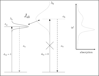
Figure 1: Schematic representation of the constituent monomers of the heterodimer. The excited states of the monomers are indicated as $\epsilon_{a}$ and $\epsilon_{b}$, correspondingly, the resonance interaction between the monomers is indicated as $J_{ab}$. The optical transition in the $a$-monomer is allowed, while it is forbidden in the $b$-monomer as indicated by the vertical black arrows. The inset shows a hypothetical absorption spectrum of such system. The position of $\epsilon_{b}$ might be above or below $\epsilon_{a}$ and therefore is shown by dotted line; reorganization energies are shown to correspond to the homogeneous linewidths of the absorption spectrum.

The constant parameters are the following: $T=300\,K$ (which corresponds to $k_{B}T\approx 208\,cm^{-1}$), $J_{ab}=100\,cm^{-1}$, $\gamma^{-1}=100\,fs$, dipole moments $d_{ag}=1,\>d_{bg}=0$ in accord with Fig. 1. The tunable parameters are the reorganization energies $\lambda_{a},\>\lambda_{b}$, given as four combinations of the values $30\,cm^{-1}$ and $150\,cm^{-1}$, and the gap between the site excitation energies with values $\pm 100\,cm^{-1}$ ("$+$" corresponds to the bright state being above the dark one; "$-$" corresponds to the opposite situation).

We will consider optical excitation as a trigger of the relaxation dynamics. The initial condition for the evolution of the RDO corresponding to a resonance excitation of the optically allowed state is then given by $\rho_{\mu\mu}(0)=|d_{\mu g}|^{2}$, where $d_{\mu g}$ is the matrix element of the transition dipole moment operator in the excitonic basis.

The main parameter characterizing a heterodimer is the difference of site energies, but as can be seen in Fig. 2, upon the presence of the bath, in the case of $\lambda_{a}\neq\lambda_{b}$, the definition of the energy gap becomes somewhat ambiguous: we can define it either as $\Delta\epsilon=\epsilon_{a}-\epsilon_{b}$ or as $\Delta\epsilon^{0}=\epsilon_{a}^{0}-\epsilon_{b}^{0}$ (even though the relation $\Delta\epsilon=\Delta\epsilon^{0}+\lambda_{a}-\lambda_{b}$ holds). Application of these different definitions of a dimeric energy gap has a distinct influence on the modeled dynamics.

Figure 2: Definition of the energy gap in the case of different reorganization energies. The dashed vertical arrows indicate the Franck-Condon transitions. Clearly $\lambda_{a}\neq\lambda_{b}$ corresponds to $\Delta\epsilon^{0}\neq\Delta\epsilon$.

3.1 Population Kinetics

We first study the dynamics of the excited state in the absence of relaxation to the ground state, i.e. when ${\cal K}=0$. In Fig. 3 we show the time evolution of the higher excitonic state population modeled by the Redfield equations (a and b), the HQME (c and d) and the secular Redfield equations (e and f) using four combinations of the reorganization energies. The left column corresponds to $\Delta\epsilon=+100\,cm^{-1}$ as a fixed energy gap, while the right column corresponds to $\Delta\epsilon^{0}=+100\,cm^{-1}$ being fixed. The equal reorganization energies (black and blue curves) serve as a good starting point for comparison of the methods. As we can see, the initial stages of the Redfield and HQME solutions ($\sim 100\,fs$) look very similar while the rates of the thermalization and the frequencies of the coherent oscillations are different (the coherent oscillations are more dramatic but shorter-lived in the Redfield solution). Moreover, different methods give us different equilibrium population values, and within the HQME solutions the latter do not coincide for two pairs of identical $\lambda$’s.

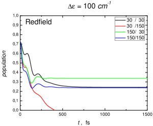
a)b)

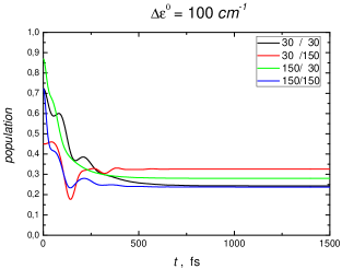
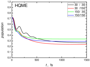
c)d)

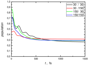
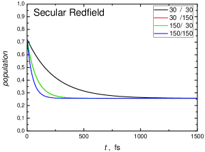
e)f)

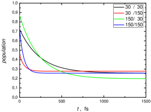
Figure 3: Evolution of the higher excitonic state population. The insets show the combination of reorganization energies given in the form $\lambda_{a}/\lambda_{b}$ ($cm^{-1}/cm^{-1}$). The left column corresponds to $\Delta\epsilon=+100\,cm^{-1},$ the right one - to $\Delta\epsilon^{0}=+100\,cm^{-1}$. a) and b), c) and d), e) and f) correspond to the full Redfield scheme, the HQME and the secular Redfield equations, respectively.

The case of different reorganization energies (red and green curves) is quite nontrivial [22]: the results for both energy gap definitions obtained by all three methods are considerably different in the long-time limit. In the right-hand column the initial values are scattered simply because fixing $\Delta\epsilon^{0}$ with different $\lambda$’s gives us different $\Delta\epsilon$ used in the definition of the excitonic basis. Moreover, the red curve in Fig. 3a reveals the well-known problem of the Redfield scheme, namely, that it does not guarantee positivity. The secular Redfield solutions do not suffer from this problem, and in this case all four $\lambda$ combinations give relaxation to the same equilibrium position.

So far we have treated the excitonic states defined by Eq. (9) as the eigenstates of the system. However, HQME solutions in the excitonic basis, as given above, exhibit non-vanishing steady state coherences. The presence of the steady state coherences can be interpreted as a reflection of renormalization of the system eigenbasis [29] taking place in the course of time. By virtue of the exact treatment of the system-bath interaction the HQME solutions are basis-independent, which allows us to identify the so-called preferred basis (or "global basis" [30]) in which the density matrix is diagonal in the long-time limit (see, e.g. [31]). This is done by diagonalizing the stationary part of the solution in the excitonic basis. Representing the RDO in the preferred basis for the fixed $\Delta\epsilon$ configuration has the effect of slightly shifting the equilibrium population values. Their order, however, remains the same as in the excitonic basis. Meanwhile for the fixed $\Delta\epsilon^{0}$ configuration (Fig. 4), we have not just quantitative but also qualitative changes in comparison with Fig. 3d. Evidently, the solutions for $\lambda_{1}\neq\lambda_{2}$ configurations now converge into the same steady state value which is in-between the ones for equal reorganization energies.

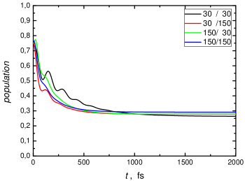
Figure 4: The HQME solution of the $\Delta\epsilon^{0}=100\,cm^{-1}$ configuration in the preferred basis. The inset shows the combination of reorganization energies given in the form $\lambda_{a}/\lambda_{b}$ ($cm^{-1}/cm^{-1}$).

3.2 Relaxation to the Ground State

We next include the relaxation to the ground state. The relaxation tensor of the equation of motion for the RDO is given by Eq. (22). We are interested in the influence of the resonance coupling on the lifetimes of the dimer eigenstates $\tau_{i}=\kappa_{i}^{-1}$. For our heterodimer we assume that in the absence of coupling the excitation of one state relaxes considerably faster than the other ($\tau_{b}\ll\tau_{a}$ or ${\cal K}_{aa,aa}\ll{\cal K}_{bb,bb}$). Therefore we can simplify Eqs. (23) to

$${\cal K}_{\alpha\alpha,\alpha\alpha}= {\cal K}_{bb,bb}\sin^{2}\theta;$$ (24)

$${\cal K}_{\beta\beta,\beta\beta}= {\cal K}_{bb,bb}\cos^{2}\theta.$$

Denoting the lifetimes of the short-lived state by $\tau_{S}\equiv\tau_{\beta}=1/{\cal{\cal K}}_{\beta\beta,\beta\beta}$ and the long-lived one by $\tau_{L}\equiv\tau_{\alpha}=1/{\cal{\cal K}}_{\alpha\alpha,\alpha\alpha}$ we present their dependence on the (site) energy gap normalized to the resonance coupling in Fig. 5. The lifetimes are normalized to the initial lifetime of the (original, i.e. uncoupled) short-lived state $\tau_{b}$.

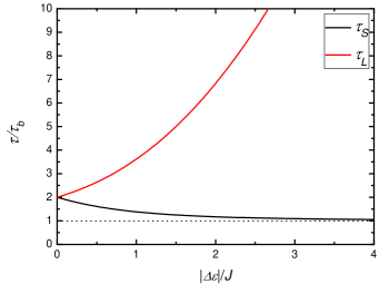
Figure 5: Excitonic mixing of lifetimes. Indices "S" and "L" denote the short-lived and the long-lived states accordingly. The energy gap $\Delta\epsilon$ is normalized to the resonance coupling, and the lifetimes are normalized to the lifetime of the short-lived state in the absence of resonance coupling ($\tau_{b}$).

Now let us consider the interplay between processes of thermalization as described in the previous subsection and relaxation to the ground state. The numerical results were obtained from the HQME with the relaxation tensor and are presented in the preferred basis. The results for a system with $\Delta\epsilon=100\,cm^{-1}$ and $\tau_{a}=2\,ns$, $\tau_{b}=5\,ps$ are shown in Fig. 6 (the corresponding "excitonic" life-times yield $\tau_{\alpha}\approx 21\,ps$ and $\tau_{\beta}\approx 7\,ps$). The populations are given in the logarithmic scale in order to reveal the two-exponential nature of the process. Only the higher state population evolutions are shown, because the lower state evolves with identical rates. The result is similar to the one shown in Fig. 4 except that instead of the steady state values we have now a decay due to relaxation to the ground state, and the long-time population values for the $\lambda_{a}\neq\lambda_{b}$ configurations (red and green curves) are no longer identical. Obviously, the long-time decay rates are identical in all four cases.

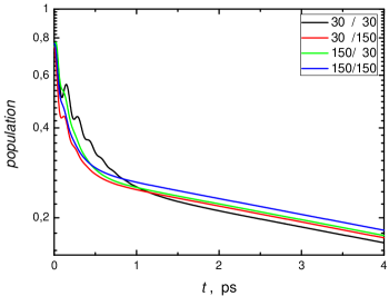
Figure 6: Solutions of the HQME with relaxation. The populations are given in the logarithmic scale. The inset shows the combination of reorganization energies given in the form $\lambda_{a}/\lambda_{b}$ ($cm^{-1}/cm^{-1}$).

To demonstrate the influence of the energetic position of the short-lived state, the evolutions for the case of $\Delta\epsilon=\pm 100\,cm^{-1}$ and $\lambda_{a}=\lambda_{b}=150\,cm^{-1}$ are considered. For demonstration, we provide an analytical approximation of the evolution while neglecting the coherent oscillations. This can be achieved by using a simple system of rate equations:

$$\begin{cases}\dot{x}=&-(\kappa_{x}+k_{x\rightarrow y})\,x\ +\ k_{y\rightarrow x}\,y;\\ \dot{y}=&-(\kappa_{y}+k_{y\rightarrow x})\,y\ +\ k_{x\rightarrow y}\,x.\end{cases}$$ (25)

Here, $x$ and $y$ are the populations (of the accordingly lower and higher states), $\kappa_{x}$ and $\kappa_{y}$ are the population relaxation rates from the tensor ${\cal K}$, and $k_{x\rightarrow y},\,k_{y\rightarrow x}$ are the effective thermalization rates obtained from the data fit of the solution of the HQME without relaxation to the ground state. Following this approach, the population of the higher state reads:

$$y(t)=C_{y1}e^{-\xi_{1}t}+C_{y2}e^{-\xi_{2}t},$$ (26)

where $\xi_{1},\>\xi_{2}$ are the eigenvalues of Eq. (25), and $C$’s are the corresponding amplitudes. When $k_{x\rightarrow y},\>k_{y\rightarrow x}\gg\kappa_{x},\>\kappa_{y}$ the second-order small terms can be neglected thus giving:

$$\begin{cases}\xi_{1}\approx&-\frac{\kappa_{x}+\kappa_{y}}{2}+\frac{(k_{x\rightarrow y}-k_{y\rightarrow x})(\kappa_{x}-\kappa_{y})}{2(k_{x\rightarrow y}+k_{y\rightarrow x})};\\ \xi_{2}\approx&-(k_{x\rightarrow y}+k_{y\rightarrow x}).\end{cases}$$ (27)

This allows us to estimate the dynamics in the following way. First, we determine quantities $C_{y1},\>C_{y2}$ and $\xi_{2}$ from the HQME solution without ${\cal K}$ (hence $\xi_{1}=0$) by numerical fitting (disregarding the oscillations). Then we derive the rates $k_{x\rightarrow y}$ and $k_{y\rightarrow x}$ from the known value of $\xi_{2}$ and the detailed balance condition. It is noteworthy that one must use an effective energy gap instead of the purely excitonic one if the reorganization energies are large. Finally, we calculate $\kappa_{x}$ and $\kappa_{y}$ from the relaxation superoperator ${\cal K}$ in the preferred basis, and then construct the $\xi_{1}$ eigenvalue.

The results obtained are depicted in Fig. 7 using the logarithmic scale. The populations of the long-lived state (in black) are shown together with their analytical approximations (in green). In the case of $\Delta\epsilon=-100\,cm^{-1}$ (dashed curves) the lower state is the long-lived one (hence, originating from the bright electronic state), therefore the thermalization part gives a minor effect. As can be seen, the actual rate of the relaxation to the ground state, $\tau$, depends on which of the two states – the short-lived or the long-lived – is the lower one in the dimer.

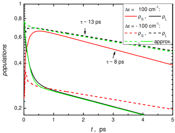
Figure 7: Solutions of the HQME with relaxation and approximations. The populations are given in the logarithmic scale. Indices "S" and "L" denote the short-lived and the long-lived states accordingly.

The analysis given above provides an explanation of the long-time decay rate ($\xi_{1}$) sensitivity to the position of the short-living state. In particular, swapping the states results in swapping the values of $\kappa_{x}$ and $\kappa_{y}$ in Eqs. (25). Therefore, the second term in the first equation from Eq. (27) changes the sign, and that is the reason why the overall decay rate is sensitive to which state – the fast decaying or the slowly decaying - is the lower one.

4 Discussion

As follows from our calculations, the asymmetry in reorganization energies allows for two non-equivalent definitions of the energy gap in the one-exciton manifold. These two cases clearly have different physical meanings. Since the energy $\epsilon$ refers to the Franck-Condon transition region of the potential energy surface (see Fig. 2), $\Delta\epsilon$ corresponds to the distance between the peak positions in the absorption spectra. Therefore we can loosely call it the "optical energy difference". This has a perfectly clear meaning in the absorption spectroscopy, however, the thermal equilibrium does not establish itself with respect to this energy gap. Should the resonance coupling be simply perturbative, we could expect the thermalization with respect to $\Delta\epsilon^{0}$ as the first approximation. Since this gap is usually used in the Förster resonance energy transfer (FRET) theory [13, 14] we shall call it the "Förster energy difference".

For the fixed optical energy difference, in the case of $\lambda_{a}=\lambda_{b}$ an equal amount of energy associated with each state is dissipated during the thermalization, and therefore the same equilibrium values are reached. In the case of $\lambda_{a}\neq\lambda_{b}$, the vibrational relaxation shifts the initial energies by a different amount ($\Delta\epsilon^{0}\neq\Delta\epsilon$). Hence, according to the Redfield relaxation, in Fig. 3a the energy gap between the states is effectively decreased (green curve) or increased (red curve) (here, the increase of the energy gap is seemingly the reason for the failure of the Redfield scheme). The case of fixed Förster energy gap (Fig. 3b) demonstrates the excitonic mixing of reorganization energies even better in the sense that for uncoupled monomers the vibrational relaxation would yield identical $\Delta\epsilon^{0}$ regardless of the combination of $\lambda$’s. The actual situation is schematically shown in Fig. 8. An interesting situation arises in the case of $\lambda_{a}<\lambda_{b}$ (Fig. 3b, red curve), because the two states are swapped in comparison with the other combinations (both initially and in the long-time limit). The way all the equilibrium values are ordered (which corresponds to the width of the energy gap that determines the equilibration) tells us the peculiarity of the Redfield scheme, namely, that the reorganization energies are mixed according to the "initial", i.e. optical energy gap (cf. Eq. (11)). Hence, the initial excitonic configuration is maintained throughout the whole evolution.

This is even more strongly pronounced in the secular Redfield scheme (Fig. 3e and f) where the equilibration is fully determined by the optical energy gap $\Delta\epsilon$ alone. This shows us how severely the neglect of the interplay between the populations and coherences can distort the picture of thermalization. For instance, it would suggest that dimers with identical absorption maxima positions but different line-widths would have identical equilibrium population distributions. The full Redfield equations, on the contrary, demonstrate that the optical energy gap, as the most intuitive input parameter, along with the resonance coupling are not enough for the description of thermal equilibrium in the case of different reorganization energies. Moreover, even the Förster energy gap can be a poor benchmark for assessing the equilibrium populations (cf. Fig. 8 bottom panel).

Figure 8: Schematic representation of the Förster energy gap in the presence of the resonance coupling. Monomeric units with identical $\Delta\epsilon^{0}$ are shown on the left. The dotted arrows on the right represent the vibrational relaxation (and tilde is used to denote the excitonic basis). The top row corresponds to $\lambda_{a}=\lambda_{b}$, the middle and the bottom ones - to $\lambda_{a}>\lambda_{b}$ and $\lambda_{a}<\lambda_{b}$ accordingly.

The HQME solutions (Fig. 3c and d) bear some resemblance to the results that follow from the Redfield equations. However, an unexpected feature is the difference between equilibrium population values for the case when $\lambda_{a}=\lambda_{b}$, which again tells us about different energy gaps in each case. This points to the action of the bath upon the system. And indeed we find that the conventional excitonic basis is just an approximate eigenbasis due to the non-vanishing coherences. Establishing the preferred basis as given previously led us to conclude that a good measure of the action of the bath is an effective resonance coupling $J_{eff}$, which has been used to replace the original $J$ value with to reproduce the effective energy gap defined by the thermal equilibrium in the eigenbasis. It appears (cf. Fig. 4) that the connection between the original resonance coupling and the effective one resembles the so-called small polaron transformation [32]. The details of such dynamic suppression of the resonance coupling captured by the HQME is beyond the scope of this paper and are presented elsewhere [30].

Discussing the relaxation to the ground state requires a couple of remarks about the excitonic mixing of lifetimes. From Eqs. (23) or (24) we notice that the mixing of lifetimes does not depend on which of the two states is the lower one. In the special case of one state being extremely long-lived, we can obtain the following picture: for a dimer degenerate in energies both excitonic states would have lifetimes twice the lifetime of the short-lived state in the site representation, whereas for different site energies in the limit of negligible coupling $J$ we retrieve the original values of the lifetimes. Now, the intermediate regime (energy gap not too big and/or rather strong resonance coupling) tells us that the shorter lifetime varies rather moderately, but the longer one can acquire a huge range of values depending on the actual arrangement of the system as demonstrated in Fig. 5.

The full picture of the excitation dissipation depends essentially on the interplay between the relaxation to the ground state and the thermalization driven by the system-bath interaction. The total process, which is a two-exponential decay, is shown in Fig. 6. The exponents can be attributed to the thermalization and relaxation to the ground state (cf. Eq. (26)). In the long-time limit, both the lower and the higher state populations decay with the same rate (the latter not shown here) because the equilibration is much faster than the relaxation. Therefore, the systems relaxes while being in a dynamic equilibrium. The reorganization energies partly determine the rates of the initial step of evolution and the amplitudes of the long-time decay. The long-time rates are identical for all four combinations of $\lambda$’s (as seen from the parallel slopes in the figure). These dependencies are qualitatively similar to those of the evolutions without relaxation to the ground state. Upon comparison of the numerical results with analytical expressions, it can be seen that the faster relaxation rate largely determines the rate of the whole process, and therefore the lifetime of the short-lived excitonic state is the determining factor of the excitation relaxation to the ground state. Moreover, as can be seen in Fig. 7 and as follows from Eqs. (27), in the presence of the system-bath interaction the decay rates are different depending on which of the two states is the lower one (cf. the case of purely excitonic mixing of lifetimes). The decay is faster if the short-lived state is below the long-lived one, however, for the parameters used, the difference is just of a few picoseconds.

The parameters of the heterodimer chosen for calculations are similar to those of the Chl–Car dimer, which is assumed to be responsible for the additional quenching of the excitation under the NPQ conditions [6]. Indeed, the excitation lifetime of the $S_{1}$ state of carotenoids is short (less than $10\,\textrm{ps}$) and the optical transition from the ground state to the $S_{1}$ state is forbidden, hence the excitation and reorganization energies in this case are not directly observable. However, the reorganization energy is a decisive parameter of the system-bath coupling, therefore, we have to consider the possible influence of the reorganization energy of the Car molecule on the excitation relaxation in such a heterodimer. It might be expected, that the excitation energy of the Car molecule in a specific Chl–Car dimer should be slightly above the excitation energy of the Chl molecule under unquenched conditions, and tends to be lower under the NPQ ones [8]. This statement can be examined using our model considerations, which demonstrate that it is only partially valid. The short lifetime component is the dominant control parameter of the excitation lifetime in such a dimer independently of the relative positioning of the molecular excitations of the monomers. As shown in Fig. 7 the excitation decays with the characteristic lifetime of $8\,\textrm{ps}$ if the optically allowed excited state of the Chl molecule is higher than the optically forbidden excited state of Car. It decays with the lifetime of $13\,\textrm{ps}$ in the opposite case. Fast (of the order of $100\,\textrm{fs}$) relaxation of the excitation from the initially excited state of the Chl molecule to the excited state of Car taking place in the former case determines the main difference between both situations. Thus, the difference in the quenching efficiency between these two cases are related to the difference in the rates of excitation transfer back to the chlorophylls of the surrounding antenna. Moreover, the dominant effect of the quenching ability of such heterodimer is determined not by the excitonic effects (see Fig. 5), but rather by the exciton-bath interaction. As can be concluded from Eqs. (27), the molecule characterized by the shortest relaxation time forms the valve of the excitation relaxation and defines the excitation lifetime within the heterodimer.

The same model of heterodimer is also applicable to exciton–CT state coupling conditions [21, 22, 25]. Since the lifetimes of both states are long and comparable, the dynamics within such a dimer corresponds to the limit of ${\cal K}=0$. The quenching ability of this dimer is determined solely by the thermalization within the excitonic states. However, Fig. 3b (or d) demonstrates that, under certain configuration of reorganization energies, the CT state can be the higher one (red curve) even though it should be the lower one to ensure the quenching ability in the Förster limit.

5 Conclusions

We have considered dynamics within a heterogeneous system of two interacting molecules. The main sources of heterogeneity in this system are the difference in excitation energies, asymmetry in reorganization energies (spectral line-widths) and the different excited state lifetimes of the chromophores. We point out that difference of reorganization energies introduces an ambiguity in the concept of energy gap between the excited states. This situation is particularly important when considering differences between coherent and incoherent transfer, since upon excitonic mixing under certain combinations of reorganization energies, the two states can become energetically swapped with respect to the uncoupled ones. Furthermore, employing the HQME technique revealed that the conventional excitonic basis becomes renormalized under the action of the bath.

The analytical study of excitonic mixing of the excited state lifetimes and the estimates following from it revealed that the lifetime of the long-living state can be indeed greatly reduced. However, we found that the final picture of energy dissipation from the system crucially depends on the system-bath interaction rather than just on the excitonic coupling. Namely, the short-living state, irrespectively of its energetic position, forms the valve of the process and largely determines the rate of dissipation by setting its lower boundary. We conclude that in the case of the Chl–Car dimer the rate of excitation relaxation is of the similar order as the inverse lifetime of Car $S_{1}$ state even if the state is above the Chl excited state. This has direct consequences in assessing the model of Chl–Car dimer as a quenching center of the NPQ process.

Appendix A Transformation of the Relaxation Superoperator

The unitary transformation of a superoperator follows from the definitions of the analogous transformation of an operator and the action of a superoperator, accordingly:

$$\tilde{\rho}=U^{-1}\rho U\;\Longrightarrow\tilde{\rho}_{ab}=\sum_{ij}(U^{-1})_{ai}\rho_{ij}U_{jb};$$ (28)

$$\tilde{\rho}={\cal U}^{-1}\rho\;\Longrightarrow\tilde{\rho}_{ab}=\sum_{cd}({\cal U}^{-1})_{ab,cd}\rho_{cd}.$$ (29)

This way any superoperator ${\cal O}$ can by transformed as $\tilde{{\cal O}}={\cal U}^{-1}{\cal O}{\cal U}$. Upon comparison of (28) and (29) we can immediately deduce a rule for composing the unitary transformation superoperator:

$$({\cal U}^{-1})_{ab,cd}=(U^{-1}\rho U)_{ab}|_{\rho_{ij}=\delta_{ic}\delta_{jd}}.$$ (30)

For instance, in the case of a heterodimer, we use Eq. (10) to obtain the following superoperator:

$${\cal U}^{-1} =\left(\begin{array}[]{cccc}c^{2}&sc&sc&s^{2}\\ -sc&c^{2}&-s^{2}&sc\\ -sc&-s^{2}&c^{2}&sc\\ s^{2}&-sc&-sc&c^{2}\end{array}\right);$$ (35)

here we use the shorthand notations: $c=\cos\theta$, $s=\sin\theta$. Therefore, bearing in mind that ${\cal K}_{ab,ab}={\cal K}_{ba,ba}=\frac{\kappa_{a}+\kappa_{b}}{2}$, it is straightforward to show that the result of a product ${\cal U}^{-1}{\cal K\,}{\cal U}$ for the population relaxation elements yields Eqs. (23).

References

- [1] A. V. Ruban, M. P. Johnson, C. D. P. Duffy, The photoprotective molecular switch in the photosystem ii antenna., Biochim. Biophys. Acta.
- [2] M. Müller, P. Lambrev, M. Reus, E. Wientjes, R. Croce, A. R. Holzwarth, Chem Phys Chem 11 (2010) 1289–1296.
- [3] P. Horton, A. Ruban, R. Walter, Annual Review of Plant Physiology and Plant Molecular Biology 47 (1996) 655–684.
- [4] N. E. Holt, D. Zigmantas, L. Valkunas, X.-P. Li, K. K. Niyogi, G. R. Fleming, Carotenoid cation formation and the regulation of photosynthetic light harvesting, Science 307 (2005) 433–436.
- [5] T. K. Ahn, T. J. Avenson, M. Ballottari, Y. C. Cheng, K. K. Niyogi, R. Bassi, G. R. Fleming, Science 320 (2008) 794–797.
- [6] S. Bode, C. C. Quentmeier, P.-N. Liao, N. Hafi, T. Barros, L. Wilk, F. Bittner, P. J. Walla, Proc. Nat. Acad. Sci. USA 106 (2009) 12311–12316.
- [7] A. V. Ruban, R. Berera, C. Ilioaia, I. H. M. van Stokkum, J. T. M. Kennis, A. A. Pascal, H. van Amerongen, B. Robert, P. Horton, R. van Grondelle, Nature 450 (2007) 575.
- [8] R. Berera, C. Herrero, I. H. M. van Stokkum, M. Vengris, G. Kodis, R. E. Palacios, H. van Amerogen, R. van Grondelle, D. Gust, T. A. Moore, A. L. Moore, J. T. M. Kennis, A simple artificial light-harvesting dyad as a model of excess energy dissipation in oxygenic photosynthesis, Proc. Nat. Acad. Sci. USA 103 (2006) 5343–5348.
- [9] P.-N. Liao, S. Pillai, D. Gust, T. A. Moore, A. L. Moore, P. J. Walla, Two-photon study on the electronic interactions between the first excited singlet states in carotenoid-tetrapyrrole dyads, J. Phys. Chem. A 115 (2011) 4082–4091.
- [10] A. Davydov, A Theory of Molecular Excitions, Mc.Graw-Hill, New York, 1962.
- [11] E. I. Rashba, M. D. Sturge (Eds.), Excitons, Elsevier, 1987.
- [12] E. A. Silinsh, V. Capek, Organic Molecular Crystals. Interaction, Localization and Transport Phenomena, AIP Press, New York, 1994.
- [13] H. van Amerogen, L. Valkunas, R. van Grondelle, Photosynthetic Excitons, World Scientific, Singapore, 2000.
- [14] V. May, O. Kühn, Charge and energy transfer in molecular systems, Wiley-VCH, 2004.
- [15] M. Cho, G. R. Fleming, The Integrated Photon Echo and Solvation Dynamics. II. Peak Shifts and 2D Photon Echo of a Coupled Chromophore, J. Chem. Phys. 123 (2005) 114506.
- [16] P. Kjellberg, B. Brüggemann, T. Pullerits, Two-dimensional electronic spectroscopy of an excitonically coupled dimer, Phys. Rev. B 74 (2) (2006) 024303.
- [17] A. V. Pisliakov, T. Mančal, G. R. Fleming, Two-dimensional optical three-pulse photon echo spectroscopy. ii. signatures of coherent electronic motion and exciton population transfer in dimer two-dimensional spectra, J. Chem. Phys. 124 (2006) 234505.
- [18] D. Abramavicius, V. Butkus, J. Bujokas, L. Valkunas, Manipulation of two-dimensional spectra of excitonically coupled molecules by narrow-bandwidth laser pulses, Chemical Physics 372 (2010) 22–32.
- [19] G. S. Schlau-Cohen, A. Ishizaki, G. R. Fleming, Two-dimensional electronic spectroscopy and photosynthesis: Fundamentals and applications to photosynthetic light-harvesting, Chem. Phys. 386 (2011) 1–22.
- [20] A. Ishizaki, G. R. Fleming, On the adequacy of the redfield equation and related approaches to the study of quantum dynamics of electronic energy transfer, J. Chem. Phys. 130 (2009) 234110.
- [21] T. Renger, Phys. Rev. Lett. 93 (2004) 188101.
- [22] T. Mančal, L. Valkunas, G. R. Fleming, Chem. Phys. Lett. 432 (2006) 301–305.
- [23] R. van Grondelle, V. I. Novoderezhkin, Energy transfer in photosynthesis: experimental insights and quantitative models, Phys. Chem. Chem. Phys. 8 (2006) 793–807.
- [24] D. J. Heijs, A. G. Dijkstra, J. Knoester, Ultrafast pump-probe spectroscopy of linear molecular aggregates: Effects of exciton coherence and thermal dephasing, Chem. Phys. 341 (2007) 230–239.
- [25] T. Mančal, L. Valkunas, E. L. Read, G. S. Engel, T. R. Calhoun, G. R. Fleming, Spectroscopy 22 (2008) 199–211.
- [26] R.-X. Xu, B.-L. Tian, J. Xu, Q. Shi, Y. Yan, Hierarchical quantum master equation with semiclassical drude dissipation, J. Chem. Phys. 131 (2009) 214111.
- [27] S. Mukamel, Principles of Nonlinear Optical Spectroscopy, Oxford University Press, New York, 1995.
- [28] A. Ishizaki, G. R. Fleming, Unified treatment of quantum coherent and incoherent hopping dynamics in electronic energy transfer: Reduced hierarchy equation approach, The Journal of Chemical Physics 130 (23) (2009) 234111.
- [29] J. Olšina, T. Mančal, Electronic coherence dephasing in excitonic molecular complexes: Role of markov and secular approximations, J. Mol. Model. 16 (2010) 1765.
- [30] A. Gelzinis, D. Abramavicius, L. Valkunas, Non-markovian effects in time-resolved fluorescence spectrum of molecular aggregates: tracing polaron formation, Phys. Rev. B (2011) submitted.
- [31] M. Schlosshauer, Decoherence and the Quantum-to-Classical Transition, The Frontiers Collection, Springer Verlag, Berlin, Germany, 2007.
- [32] A. H. Romero, D. W. Brown, K. Lindenberg, Phys. Rev. B 59 (1999) 13728–13740.