Excited meson spectroscopy with two chirally improved quarks

Abstract:

The excited isovector meson spectrum is explored using two chirally improved dynamical quarks. Seven ensembles, with pion masses down to $\approx$ 250 MeV are discussed and used for extrapolations to the physical point. Strange mesons are investigated using partially quenched s-quarks. Using the variational method, we extract excited states in several channels and most of the results are in good agreement with experiment.

1 Introduction

The bulk of experimental knowledge about QCD observables is contained in the hadron spectrum, listed by the Particle Data Group [1]. So far, lattice QCD is the only known technique to perform corresponding ab-initio calculations. We use the Chirally Improved Dirac operator [2], an approximate solution of the Ginsparg-Wilson (GW) equation [3]. We present results for ground and excited states of the isovector mesons in 2-flavor QCD, making use of the variational method. We access strange mesons by including partially quenched strange quarks in the analysis. Recent preceeding work was published in [4, 5, 6]. A more extensive discussion of the results will be found in [7].

2 Simulation details

The simulation method is detailed in [8]. The Chirally Improved Dirac operator ($D_{\textrm{\scriptsize{CI}}}$) is obtained by plugging the most general ansatz for a Dirac operator into the GW equation and comparing the coefficients. Furthermore, one level of stout smearing enters the definition of $D_{\textrm{\scriptsize{CI}}}$, and the Lüscher-Weisz gauge action is used. We generate the dynamical configurations with a Hybrid Monte-Carlo (HMC) algorithm. We simulate seven ensembles with lattices of size $16^{3}\times 32$, for details see Table 1.

set	$m_{\pi}$[MeV]	$a$[fm]	$\beta_{LW}$	$m_{0}$	$m_{\pi}L$	configs
A50	596(7)	0.1324(11)	4.70	-0.050	6.40	200
A66	255(7)	0.1324(11)	4.70	-0.066	2.72	200
B60	516(6)	0.1366(15)	4.65	-0.060	5.72	300
B70	305(6)	0.1366(15)	4.65	-0.070	3.38	200
C64	588(6)	0.1398(14)	4.58	-0.064	6.67	200
C72	451(5)	0.1398(14)	4.58	-0.072	5.11	200
C77	330(5)	0.1398(14)	4.58	-0.077	3.74	300

Table 1: Parameters used in the simulation of the seven ensembles. Given are the pion mass $m_{\pi}$, the lattice spacing $a$, the gauge coupling parameters $\beta_{LW}$, the quark mass parameters $m_{0}$, the factor $m_{\pi}L$ with the spatial extent $L$ of the lattice and the number of (approximately independent) configurations. The lattice spacing is set using the static potential assuming a Sommer parameter of $r_{0,exp}=0.48\,$ fm, detailed in the text.

The variational method [9, 10] is applied to extract ground and excited states. The correlation matrix for a given set of interpolators is

$$C_{ij}(t) = \langle 0|O_{i}(t)O_{j}^{{\dagger}}|0\rangle=\sum_{k=1}^{N}\langle 0|O_{i}|k\rangle\langle k|O_{j}^{{\dagger}}|0\rangle\,\mathrm{e}^{-tE_{k}}.$$ (1)

The idea of the variational method is to offer a basis of suitable interpolators, from which the system chooses the linear combinations closest to the physical eigenstates $|k\rangle$. The generalized eigenvalue equation

$$C(t)\,\vec{v}_{k} = \lambda_{k}(t,t_{0})\,C(t_{0})\,\vec{v}_{k}\;,\qquad\lambda_{k}(t,t_{0})\propto\mathrm{e}^{-(t-t_{0})\,E_{k}}\left(1+\mathcal{O}(\mathrm{e}^{-(t-t_{0})\,\Delta E_{k}})\right)\ ,$$ (2)

gives the energies of the eigenstates, where $\Delta E_{k}$ is the difference between $E_{k}$ and its closest energy level. The eigenvectors represent the linear combinations of the used set of interpolators which are close to the physical states related to the eigenvalues. We use two Gaussian (narrow and wide) and derivative sources. The Gaussian sources are obtained using gauge-covariant Jacobi smearing, the derivative source by applying the covariant derivative on the wide source. Combining these quark sources, several interpolators are constructed in each hadron channel. All sources are located in single time slices, built on configurations which are hypercubic-smeared (HYP) in the spatial directions three times. Complete tables of interpolators will be found in the Appendix of [7] and differ slightly from [5]. We consider isovector-mesons, which are free of disconnected diagrams. Within our present framework, isoscalars can be discussed only with the systematic error of neglected disconnected diagrams. We use the meson interpolator construction as described in [11], which is similar to constructions previously used in [12, 13, 14].

In order to set the scale, the dimensionless lattice observable $a/r_{0}$ (cf. Table 1) is extrapolated linearly in $(am_{\pi})^{2}$ for ensembles sharing the same gauge coupling. We extrapolate to the physical value of the dimensionless product $m_{\pi}r_{0}$ (represented by a parabola in this specific graph). This procedure defines a scale for each gauge coupling, independent of the particular quark mass parameters, where physical input is used only at the physical point.

3 Results

3.1 The light 0^-+ channel: $\pi$

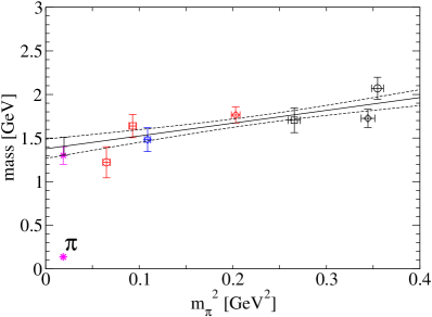
Figure 1: Mass plot for the $0^{-+}$ channel ($\pi$), first excitation. The ground state defines the abscissa.

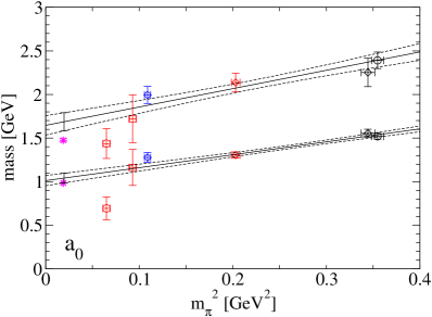
Figure 2: Mass plot for the 0⁺⁺ channel ($a_{0}$), ground state and first excitation.

As usual, the pion ground state mass is used as scale for the chiral extrapolation for all other observables. For the first excitation we use the set of operators (1,2,17). Due to the finiteness of the lattice, the backrunning pion limits the possible fit range for the first excitation, in particular at small pion masses (see Fig. 2). Nevertheless, masses can be extracted and the chiral extrapolation hits the experimental $\pi(1300)$ within $1\sigma$ (see Fig. 2).

3.2 The light 0⁺⁺ channel: $a_{0}$

In the 0⁺⁺ channel, we extract the ground state and the first excited state using the set of interpolators (10,12,13). The energy levels of ensemble A66 appear unexpectedly light (see Fig. 2), which may be related to scattering states becoming visible in the analysis at light sea quark masses. Thus, we cannot exclude sizeable contributions from the two-particle state $\pi\eta_{2}$. However, the chiral extrapolations – dominated by the larger pion mass data – are compatible with the experimental one-particle states $a_{0}(980)$ within 1$\sigma$ and with $a_{0}(1450)$ within 1$\sigma$. Due to the comparatively small value of $m_{\pi}L$ for A66 there may be a significant finite size effect, as well.

3.3 The strange 0^- channel: $K$

Figure 3: Mass plot for the strange 0^- channel ($K$), ground state and first excitation.

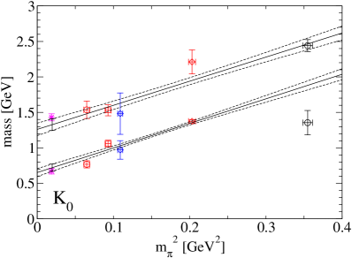
Figure 4: Mass plot for the strange 0⁺ channel ($K_{0}^{*}$), ground state and first excitation.

In the strange $0^{-{}}$ channel, interpolator (1) is used for the ground state and interpolators (1,2,8,17) for the excited state. The extrapolated masses are close to the experimental ground state and the $K(1460)$ (see Fig. 4), confirming the latter, which is omitted from the summary table of [1].

3.4 The strange 0⁺ channel: $K_{0}^{*}$

The $K_{0}^{*}(800)$ is a very broad resonance, omitted from the summary table of [1]. We use the interpolators (10,12,13) in A50 and C72 and (4,10,12,13) in A66, B70 and C77, i.e., at small pion masses. In B60 and C64 the signals are too noisy to produce a reliable value. The chiral extrapolations are compatible with the $K_{0}^{*}(800)$ and the $K_{0}^{*}(1430)$ (see Fig. 4).

3.5 The light 1^– channel: $\rho$

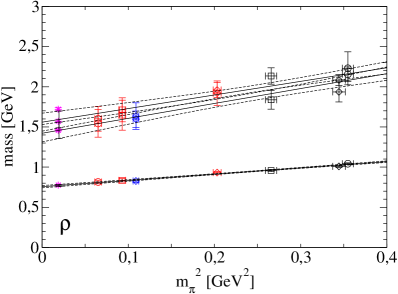
Figure 5: Mass plot for the 1^– channel ($\rho$), ground state and two excitations.

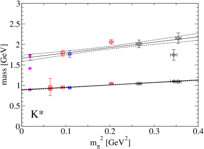
Figure 6: Mass plot for the strange 1^- channel ($K^{*}$), ground state and first excitation.

The $\rho(770)$ comes out nicely as usual. The excitations are extracted using subsets of the interpolators (1,8,12,17,18,20,22). The excitations are very close (see Fig. 6). However, the eigenvectors do not confirm this picture. Therefore, we extrapolate the results according to the naïvely assumed level ordering. The results are compatible with the experimental $\rho(1450)$ and $\rho$(1700 or 1570) within error bars.

3.6 The strange 1^- channel: $K^{*}$

In the strange $1^{-{}}$ channel, we use the set (1,8,9), which includes both types of approximate $C$-parities. The ground state comes out nicely and is dominated by the $[C\approx-]$ interpolators. For the first excitation, we find hardly any mixing at large pion masses, but some mixing in ensemble A66. The corresponding A66 excited energy level is almost degenerate with the ground state, which remains a puzzle (see Fig. 6). Due to its rather large error bar, the chiral extrapolation of the excitation still hits the $K^{*}(1680)$. Our results suggest that simulations at smaller pion masses and with higher statistics are necessary in order to reliably describe the mixing of different $C$-parities and to be able to obtain the $K^{*}(1410)$.

3.7 The light 1⁺⁺ channel: $a_{1}$

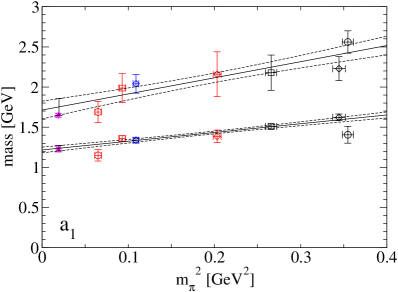
Figure 7: Mass plot for the 1⁺⁺ channel ($a_{1}$), ground state and first excitation.

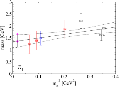
Figure 8: Mass plot for the exotic 1^-+ channel ($\pi_{1}$), ground state.

In the 1⁺⁺ channel ($a_{1}$), the ground state is extracted using the single interpolator (1), the first excitation using subsets of (1,2,4,13,15). Some of the plateaus drop slightly at large time separations. which may be a hint that the true ground state is not reached in our fit interval. Nevertheless, the chiral extrapolations hit the experimental $a_{1}(1260)$ and the $a_{1}(1640)$ within error bars (see Fig. 8). We thus confirm the existence of the latter, which is omitted from the summary table of [1].

3.8 The light 1^-+ channel: $\pi_{1}$

Due to the weak signal in the exotic $1^{-{+}}$ channel ($\pi_{1}$), the choice of operators is optimized in each ensemble separately. Doing so, a mass can be extracted, albeit with comparatively large statistical uncertainty (see Fig. 8). The chiral extrapolation hits the experimental $\pi_{1}(1400)$, but is also compatible with the $\pi_{1}(1600)$.

3.9 The light 2⁺⁺ channel: $a_{2}$

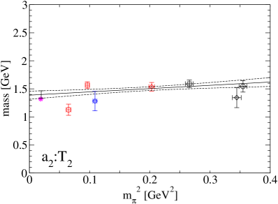
Figure 9: Mass plot for the 2⁺⁺ channel ($a_{2}$), ground state in representation T₂.

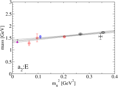
Figure 10: Mass plot for the 2⁺⁺ channel ($a_{2}$), ground state in representation E.

In the $2^{+{+}}$ channel ($a_{2}$), interpolator (2) in $T_{2}$ and (2) (respectively (6) in A66) in $E$ is used to extract the ground state. Some of the plateaus appear to be lighter than expected (see Figs. 10 and 10), however, the deviations being in a range which is compatible with statistical fluctuations. The chiral extrapolations of the orthogonal lattice representations $T_{2}$ and $E$ agree and match the experimentally known resonance $a_{2}(1320)$ within error bars.

4 Conclusions

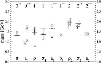
Figure 11: Collection of the mass results for light and strange mesons (left to right), obtained by chiral extrapolation of dynamical light quarks linear in the pion mass squared. Experimental values listed by the Particle Data Group [1] are denoted by horizontal lines, dashed lines indicate needed confirmation. Results shown side by side stem from different sets of interpolators (resp. $T_{2}$ and $E$ in spin 2). Strange quarks are analyzed in the partial quenching approximation. Isoscalars suffer from neglected disconnected diagrams.

We presented results for the excited meson spectrum from two dynamical Chirally Improved quarks. Seven ensembles with pion masses in the range of 250 to 600 MeV have been analyzed. Strange mesons have been treated in the partially quenched approximation. The majority of results agrees well with experiment (see Fig. 11), some states can be confirmed which are omitted from the summary table of the Particle Data Group [1].

- [1] K. Nakamura et al., Review of particle physics, J. Phys. G 37 (2010) 075021.
- [2] C. Gattringer, A new approach to Ginsparg-Wilson fermions, Phys. Rev. D 63 (2001) 114501, [hep-lat/0003005]. C. Gattringer, I. Hip and C.B. Lang, Approximate Ginsparg-Wilson fermions: A first test, Nucl. Phys. B 597 (2001) 451, [hep-lat/0007042].
- [3] P. H. Ginsparg and K. G. Wilson, A remnant of chiral symmetry on the lattice, Phys. Rev. D 25 (1982) 2649.
- [4] G. P. Engel, C. Gattringer, C. B. Lang, M. Limmer, D. Mohler, and A. Schäfer, Excited hadrons in =2 QCD, PoS LAT09 (2009) 088, [arXiv:0910.2802].
- [5] G. P. Engel, C. B. Lang, M. Limmer, D. Mohler, and A. Schäfer, Meson and baryon spectrum for QCD with two light dynamical quarks, Phys. Rev. D 82 (2010) 034505, [arXiv:1005.1748].
- [6] G. P. Engel, C. B. Lang, M. Limmer, D. Mohler, and A. Schäfer, Some results on excited hadrons in 2-flavor QCD, PoS LATTICE2010 (2010) 103, [arXiv:1010.2366].
- [7] G. P. Engel, C. B. Lang, M. Limmer, D. Mohler, and A. Schäfer, in preparation.
- [8] C. Gattringer, C. Hagen, C. B. Lang, M. Limmer, D. Mohler, and A. Schäfer, Hadron spectroscopy with dynamical chirally improved Fermions, Phys. Rev. D 79 (2009) 054501, [arXiv:0812.1681].
- [9] C. Michael, Adjoint sources in lattice gauge theory, Nucl. Phys. B 259 (1985) 58.
- [10] M. Lüscher and U. Wolff, How to calculate the elastic scattering matrix in 2-dimensional quantum field theories by numerical simulation, Nucl. Phys. B 339 (1990) 222.
- [11] C. Gattringer, L. Y. Glozman, C. B. Lang, D. Mohler, and S. Prelovsek, Derivative sources in lattice spectroscopy of excited mesons, Phys. Rev. D 78 (2008) 034501, [arXiv:0802.2020].
- [12] P. Lacock, C. Michael, P. Boyle, and P. Rowland, Orbitally excited and hybrid mesons from the lattice, Phys. Rev. D 54 (1996) 6997, [hep-lat/9605025].
- [13] X. Liao and T. Manke, Excited charmonium spectrum from anisotropic lattices, (2002) [hep-lat/0210030].
- [14] J. J. Dudek, R. G. Edwards, N. Mathur, and D. G. Richards, Charmonium excited state spectrum in lattice QCD, Phys. Rev. D 77 (2008) 034501, [arXiv:0707.4162].