Effects of confinement on thermal stability and folding kinetics in a simple Ising–like model

Abstract

In cellular environment, confinement and macromulecular crowding play an important role on thermal stability and folding kinetics of a protein. We have resorted to a generalized version of the Wako–Saitô–Muñoz–Eaton model for protein folding to study the behavior of six different protein structures confined between two walls. Changing the distance $2R$ between the walls, we found, in accordance with previous studies, two confinement regimes: starting from large $R$ and decreasing $R$, confinement first enhances the stability of the folded state as long as this is compact and until a given value of $R$; then a further decrease of $R$ leads to a decrease of folding temperature and folding rate. We found that in the low confinement regime both unfolding temperatures and logarithm of folding rates scale as $R^{-\gamma}$ where $\gamma$ values lie in between $1.42$ and $2.35$.

protein folding; spatial confinement; Wako–Saitô–Muñoz–Eaton model

1 Introduction

In the past the majority of experiments on protein folding have been carried out in diluted solutions but in the last two decades it has become clear that these experiments do not take into account two issues which arise in vivo and whose relevance on thermal stability and equilibrium rates is not negligible. Namely, crowding and confinement [1, 2, 3, 4]. Crowding refers to the fact that about 30% of cells internal volume is occupied by macromolecules such as lipids, carbohydrates and proteins themselves [1]. This fraction could even reach 40% in E. Coli [5]. Confinement is merely a limitation in the volume available to the polypeptide chain as naturally occurs in the exit tunnel of ribosomes or in the chaperonin cavity.

Studying protein folding properties in a crowded environment is experimentally possible simply by adding high concentrations of macromolecules to solutions, but this approach has problems because of specific interactions which arise between proteins and crowding agents and because crowding promotes protein–protein aggregation [1]. Based on the idea that the main effect of crowding is the reduction of volume available to the protein due to steric constraints, theoretical studies and simulations have shown that crowding may be quantitatively mapped onto confinement as long as crowding agents are modelled as hard spheres and the volume fraction occupied by them does not exceed $10$% [6]. Thanks to this mapping, experimental and theoretical studies on confinement may give many hints also for crowding effects. However the above conditions often does not hold in the cell interior because of too high concentration of agents or presence of macromolecules–protein attractive interaction. In addition, gradients in macromolecule concentrations may exist [7] and, from a more general point of view, crowding is dynamic in nature whereas confinement is static. Thus, the mapping is not close enough to draw a completely satisfactory analogy between crowding and confinement.

An experimental procedure to mimic the effects of confinement, is the encapsulation of proteins within pores of silica gels [8, 9] or glasses [10] or polyacrylamide gels [11]. These experiments reported, for most of the considered proteins, an increase in thermal stability when they are confined into nanopores. Melting temperature ($T_{\mbox{\footnotesize{f}}}$) shift is even dramatic in the cases of $\alpha$–lactalbumin and RNase A, being as large as about $30$ K [8, 10]. On the contrary, recent experiments suggested that crowding influence on stability is modest [7, 12].

The commonly accepted reason for the increase in stability is the change in conformational entropy induced by confinement [13, 14, 15, 16, 17, 18]. Encapsulating the protein in a given volume disallows the most expanded configurations of the denatured state ensemble and so indirectly favours more compact structures and, among them, the folded state. The same argument explains also why confinement should lead to an increase in folding rates $k_{\mbox{\footnotesize{f}}}$ as long as the nanopore size is large enough to contain the folded state and to permit chain reconfigurations around it [13, 14, 15, 16, 17, 18, 19].

From polymer physics we know that a polymer confined between two (sufficiently close) inert hard walls, behaves like a pancake with the radius of gyration (parallel to the walls) that scales as a power of the number of monomers [20, 21, 22]. Furthermore, when it is confined within a cage with repulsive walls, its free energy follows a simple power law dependence on the size of the cage $R$ [20, 21]. Then, as shown by Takagi et al. [17], folding temperatures and rates should follow the scaling laws $\Delta T_{\mbox{\footnotesize{f}}}\sim\Delta\ln k_{\mbox{\footnotesize{f}}}\sim R^{-\gamma}$.

Literature reports many values for the exponent $\gamma$: for an ideal gaussian chain confined between two walls ($d_{\mbox{\footnotesize{c}}}=1$), in a cylinder ($d_{\mbox{\footnotesize{c}}}=2$) or in a spherical cavity ($d_{\mbox{\footnotesize{c}}}=3$), $\gamma=2$ while for an excluded volume chain $\gamma=5/3$ for $d_{\mbox{\footnotesize{c}}}=1,2$ and $\gamma=15/4$ for $d_{\mbox{\footnotesize{c}}}=3$. Using a Gō–model $\alpha$–carbon representation of proteins and Langevin simulations in a cylindrical cage, Takagi et al. [17] found $\gamma=3.25\,\pm\,0.09$. Best and Mittal [18] simulated confinement of protein G and a $3$–helix bundle in different geometries and reported that for $d_{\mbox{\footnotesize{c}}}=1,2$ both values $\gamma=2$ and $\gamma=5/3$ are a good estimate of the behavior of the two proteins, but they also remarked the fact that it is hard to distinguish which value fits best the simulations because least square fitting of power laws can produce biased estimates of parameters for small samples. For spherical confinement the same authors reported a behavior which is stronger than $\gamma=2$ but much weaker than expected behavior for the excluded volume chain ($\gamma=15/4$).

In the present work we confine a simple Ising–like model (WSME model) originally proposed by Wako and Saitô in 1978 and later reconsidered by Muñoz and Eaton [23, 24, 25, 26, 27]. Equilibrium thermodynamics of the model can be solved exactly [28]. The cluster variation method is exact for this model [29] and it successfully describes the kinetics of protein folding [30, 31, 32, 33]. More recently it has been proposed a generalized version of the model that permits to reproduce the general features of mechanical unfolding [34, 35] and, through Monte Carlo simulations, to obtain for some already widely studied proteins and RNA fragments, unfolding pathways which are consistent with results of experiments and/or of simulations made with more detailed models [36, 37, 38, 39]. The model has also been used with success to study folding equilibrium and kinetics and to mimic mutations of a small ankyrin repeat protein [40].

We use the confined WSME model to study thermodynamics and kinetics of three ideal structures and three simple proteins in confining conditions. The ideal structures are a $10$ residues ideal $\alpha$–helix, a $2$–stranded and a $3$–stranded ideal $\beta$–sheets each with $7$ residues per strand. Real structures are a $3$–helix bundle, protein G and its C–terminal $\beta$–hairpin. The paper is organized as follows: in Sec. 2 we describe the WSME model and its confinement. Sec. 3.1 focuses on the confinement–induced changes of thermodynamic stability for the different proteins while Sec. 3.2 deals with kinetics and the expected increase in folding rates. Some conclusions are drawn in Sec. 4.

2 The model

WSME model is a Gō–like model in which a given $N$ residues protein is described by a sequence of $N$ binary variables $m_{k}$, whose value is $1$ if $k$–th residue is in the native configuration and $0$ otherwise. Two residues interact only if they and all residues between them are native and only if they are in contact in the native structure, i.e. they have at least a pair of atoms which are closer than the threshold length of $4$ Å in the native structure. If residues $i$ and $j$ are in contact in the native structure we associate to them a negative energy $-\varepsilon_{ij}$ (defined as in [27]) and a contact matrix element $\Delta_{ij}=1$. If the two residues are not in contact $\Delta_{ij}=0$. When the molecule is pulled at its ends by a constant force $f$, the Hamiltonian reads:

$$H\left(\{m_{k}\},\{\sigma_{ij}\}\right)=-\sum_{i=1}^{N-1}\sum_{j=i+1}^{N}\varepsilon_{ij}\Delta_{ij}\prod_{k=i}^{j}m_{k}-fL$$ (1)

where $L=L\left(\{m_{k}\},\{\sigma_{ij}\}\right)$ is the end–to–end length of the protein and $\{\sigma_{ij}\}$ is a set of new binary variables that will soon be defined and in which the greater entropy of non–native states is encoded.

Here and in the following we define a native stretch from residue $i$ to residue $j$ as a sequence of native residues delimited by the two non–native residues $i$ and $j$. The end–to–end length $L$ is the sum of the native stretches lengths $l_{ij}$ multiplied by a sign $+1$ or $-1$ (the binary variable $\sigma_{ij}$) if the stretch is parallel or antiparallel to the direction of the force. The binary variable $\sigma_{ij}$ thus represents the direction of the stretch from $i$–th to $j$–th residue. Using the quantity $S_{ij}=(1-m_{i})m_{i+1}\ldots m_{j-1}(1-m_{j})$, which is equal to $1$ if the sequence of residues from $i$ to $j$ is a native stretch and is $0$ otherwise, and setting the boundary conditions $m_{0}=m_{N+1}=0$, the length $L$ is defined as:

$$L\left(\{m_{k}\},\{\sigma_{ij}\}\right)=\sum_{i=0}^{N}\sum_{j=i+1}^{N+1}\sigma_{ij}l_{ij}S_{ij}$$ (2)

The set of all possible lengths $\{l_{ij}\}$ is obtained directly from the three dimensional structure deposited in the Protein Data Bank (pdb) as the distances between the various pairs of central carbon atoms $\{\mbox{C}_{\alpha_{i}},\mbox{C}_{\alpha_{j}}\}$. Besides $l_{ij}$, other two lengths associated to the stretch from the $i$–th to the $j$–th residue are important for what follows. These are the maximum $p_{ij}^{\mbox{\scriptsize{max}}}$ and the minimum $p_{ij}^{\mbox{\scriptsize{min}}}$ among the distances between $\mbox{C}_{\alpha_{i}}$ and the projections of each $\mbox{C}_{\alpha_{k}}$ ($i\leq k\leq j$) on the straight line from $\mbox{C}_{\alpha_{i}}$ to $\mbox{C}_{\alpha_{j}}$. Note that, as shown in figure 1 (axis $x2$), $p_{ij}^{\mbox{\scriptsize{max}}}\geq l_{ij}$ and $p_{ij}^{\mbox{\scriptsize{min}}}\leq 0$.

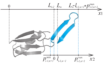
Figure 1: Sketch of a configuration with residue $m_{i-1}=0$. Axis $x1$ shows relevant lengths of entire molecule. Axis $x2$ shows relevant lengths of native stretch from ($i-1$)–th to ($n+1$)–th residues.

The constrained zero–force partition function

$$Z(L;f=0)=\sum_{\{m_{k}\}}\sum_{\{\sigma_{ij}\}}\delta\left(L-L(\{m_{k}\},\{\sigma_{ij}\})\right)e^{-\beta H\left(\{m_{k}\},\{\sigma_{ij}\};f=0\right)}$$ (3)

can be recursively calculated building up the protein residue by residue and evaluating at each step the partition function $z_{n}(L)$, where $n$ is the number of residues achieved at that step (see appendix of [35] for detailed calculations).

$$\left\{\begin{array}[]{l}a_{n}^{i}(L)=e^{\beta\chi_{in}}\left[z_{i-2}(L-l_{i-1,n+1})+z_{i-2}(L+l_{i-1,n+1})\right]\\ \\ z_{n}(L)=\sum_{i=1}^{n+1}a_{n}^{i}(L)\end{array}\right.$$ (4)

Where $\chi_{in}=\sum_{k=i}^{n-1}\sum_{r=k+1}^{n}\varepsilon_{kr}\Delta_{kr}$ is minus the energy of the native stretch from ($i-1$)–th to ($n+1$)–th residue and the initial conditions are $z_{-1}(L)=1$ for $L=0$ and $z_{-1}(L)=0$ for $L\neq 0$. The goal of the recursive scheme is the constrained partition function $Z(L;f=0)$ which corresponds to $z_{N}(L)$. The absolute value of the possible end–to–end lengths of a protein cannot be greater than $L_{\mbox{\footnotesize{max}}}=\sum_{i=0}^{N}l_{i,i+1}$, which corresponds to the length of the molecule in the completely unfolded, fully extended configuration. Thus, because of finite resolution of amino acids coordinates in the pdb file (which is $10^{-3}$ Å), $L$ belongs to a finite set of values in the range $\left[-L_{\mbox{\footnotesize{max}}},L_{\mbox{\footnotesize{max}}}\right]$.

2.1 Confinement of WSME model

Consider again the recursive scheme of (4) and set the starting point of the molecule in the middle of the cage. In order to confine the protein into a cage of size $2R$ with perfectly repulsive walls, when adding a native stretch from ($i-1$)–th to ($n+1$)–th residues (which are respectively at the distances $L_{i-2}$ and $L_{n}$ from the N–terminus), one has to require that every residue of this stretch lie inside the cage. This issue may be solved by considering also the lengths $p_{i-1,n+1}^{\mbox{\scriptsize{max}}}$ and $p_{i-1,n+1}^{\mbox{\scriptsize{min}}}$ of the native stretch (see axis $x1$ of figure 1) and inserting appropriate step functions in the recursive scheme:

$$\left\{\begin{array}[]{l}\begin{array}[]{lcl}a_{n}^{i}(L)&=&e^{\beta\chi_{in}}\;\times\\ \end{array}\\ \quad\times\;\left[z_{i-2}(L-l_{i-1,n+1})\theta(R-L+l_{i-1,n+1}-p_{i-1,n+1}^{\mbox{\scriptsize{max}}})\theta(R-l_{i-1,n+1}+L+p_{i-1,n+1}^{\mbox{\scriptsize{min}}})+\right.\\ \quad\left.+z_{i-2}(L+l_{i-1,n+1})\theta(R+L+l_{i-1,n+1}-p_{i-1,n+1}^{\mbox{\scriptsize{max}}})\theta(R-l_{i-1,n+1}-L+p_{i-1,n+1}^{\mbox{\scriptsize{min}}})\right]\\ \\ z_{n}(L)=\sum_{i=1}^{n+1}a_{n}^{i}(L)\end{array}\right.$$ (5)

where $\theta$ is the Heaviside step function:

$$\theta(x)=\left\{\begin{array}[]{ll}1&\mbox{ if }x\geq 0\\ 0&\mbox{ else }\end{array}\right.$$

Translational freedom must also be taken into account. To this end, for a given configuration, instead of considering simply the end-to-end length, it would be better to consider as the relevant length the distance between the two farthest residues of that configuration. We call it the configuration effective length. Fixing in the center of the cage the N–terminus excludes from the partition functions $z_{n}(L)$ the contribution of some of the configurations which have an effective length shorter than $2R$ (for example in fig. 2a configuration $a1$ has an effective length shorter than configuration $a2$ but the former is forbidden while the latter is allowed).

Figure 2: Three different configurations which would give a contribution to the partition function constrained at length $L$ without any cage. With cage a only configurations $2$ and $3$ contribute. In b only configurations $1$ and $3$ contribute.

Thus, to take into account all the configurations with an effective length shorter than the cage size, the partition function has to be computed for different positions of the cage relative to the N–terminus. The final partition function will be the sum of various partition functions at different cage positions. Note that some configurations will appear many times in such a scheme (for example state $a3$ of fig. 2a) as a consequence of their greater translational freedom.

To obtain the final partition function one has to repeat this procedure considering all the possible positions of the cage relative to the N–terminus, i.e. to start with the range $\left[-2R,0\right]$ and to move the cage with a step $\Delta R$ equal to the resolution of the $\{l_{ij}\}$ until the final range $\left[0,2R\right]$ is reached. To speed up computations we rounded the lengths to a resolution of $10^{-1}$ Å  . For the $3$–helix bundle we checked that this assumption does not modify the results through a comparison with results obtained at the resolution of $10^{-3}$ Å.

3 Results and discussion

3.1 Equilibrium

In this study we considered six different structures. Three are real structures: a $3$–helix bundle (pdb code 1PRB), protein G (pdb code 2GB1) and its final hairpin. The other three structures are an ideal $\alpha$–helix of ten residues (radius $2.3$ Å, pitch $5.4$ Å, $\varepsilon_{ij}=1$ if $j=i+4$ and $\varepsilon_{ij}=0$ otherwise), a $2$–stranded and a $3$–stranded antiparallel $\beta$–sheets with $7$ residues in each strand (the $3$–stranded sheet is drawn in figure 3).

Figure 3: Ideal antiparallel $\beta$–sheet with $3$ strands. Distance between two consecutive residues is $3.8$ Å. Dashed lines represent active contacts. For them $\varepsilon_{ij}=1$, while $\varepsilon_{ij}=0$ in other cases.

In the following, code ‘a010’ refers to the ideal $\alpha$–helix, ‘b207’ and ‘b307’ to the two $\beta$–sheets which have respectively $2$ and $3$ strands and ‘GB1h’ refers to the final hairpin of protein G.

To study the equilibrium response to confinement of the six structures, we computed, at different cage sizes $R$, thermodynamic quantities as the Helmholtz free energy, the specific heat and the average fraction of native residues. For each structure we varied the distance $2R$ between the walls, in a range from about the mininum effective length of the completely unfolded state to twice the maximum length of the completely unfolded state, i.e. from $4$ Å  (the distance between two subsequent amino acids is about $3.8$ Å) to $2L_{\mbox{\footnotesize{max}}}$.

If we denote with $L_{\mbox{\scriptsize{N }\footnotesize{eff.}}}$ the effective length of the native state (values are reported in table 1), we may naively distinguish between two different confinement regimes: (i) one, for $2R>L_{\mbox{\scriptsize{N }\footnotesize{eff.}}}$, which disallows the more expanded conformations of the non–native basin but not the folded state, and (ii) the strong confinement regime, for $2R<L_{\mbox{\scriptsize{N }\footnotesize{eff.}}}$, which forbids also the fully native state.

Table 1 also shows the effective length of the unfolded state $L_{\mbox{\scriptsize{U }\footnotesize{eff.}}}$. This is obtained through a Monte Carlo simulation at the unfolding temperature as the average effective length over the configurations belonging to the unfolded basin. Details about Monte Carlo moves will be given in the next section.

Table 1: Native state end–to–end length ($L_{\mbox{\scriptsize{N}}}$), effective length of the native state ($L_{\mbox{\scriptsize{N }\footnotesize{eff.}}}$), maximum length of the fully unfolded state ($L_{\mbox{\footnotesize{max}}}$) and effective length of the unfolded state ($L_{\mbox{\scriptsize{U }\footnotesize{eff.}}}$) for the six different structures.

• 	a010	b207	b307	GB1h	1PRB	2GB1
  $L_{\mbox{\scriptsize{N}}}$ (Å)	$14.3$	$3.8$	$24.0$	$6.5$	$40.0$	$27.8$
  $L_{\mbox{\scriptsize{N }\footnotesize{eff.}}}$ (Å)	$14.3$	$3.8$	$24.0$	$6.6$	$40.0$	$29.1$
  $L_{\mbox{\footnotesize{max}}}$ (Å)	$34.2$	$49.4$	$76.0$	$63.8$	$201$	$212$
  $L_{\mbox{\scriptsize{U }\footnotesize{eff.}}}$ (Å)	$14.1$	$21.8$	$27.3$	$24.1$	$40.5$	$46.3$

Since, without confinement, for a given set of binary variables $\{m_{k}\}$, the model admits $2^{\sum_{i=1}^{N}(1-m_{i})}$ configurations and this number grows exponentially with the amount of non–native residues, we may expect that confinement in a cage of size $R$, with $L_{\mbox{\footnotesize{max}}}>2R>L_{\mbox{\scriptsize{N }\footnotesize{eff.}}}$, gives a reduction of conformational entropy which affects more the non–native basin. Besides, one has to consider translational freedom whose role is to further stabilize the most compact configurations irrespectively of the fact that they belong or not to the native basin. Thus a structure with $L_{\mbox{\scriptsize{N }\footnotesize{eff.}}}>L_{\mbox{\scriptsize{U }\footnotesize{eff.}}}$, as in the case of the ideal $\alpha$–helix, does not undergo any stabilization of the folded state. Figure 4 shows the free energy landscapes for the three real structures at different confinement sizes (for a better comparison the free energy of the completely folded state has always been set to zero). For the final hairpin of protein G confinement increases the free energy of both the native and non–native basin: both native and non–native basin are destabilized but the latter is more affected. On the contrary, for the $3$–helix bundle both native and non–native basins are stabilized, with a slightly greater stabilization with confinement for the native state. Finally, for protein G, only the non–native basin is destabilized by confinement.

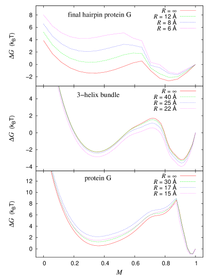
Figure 4: Free energy profile in function of the fraction of native residues $M$ at various confinement radius $R$ for the $3$–helix bundel, protein G and its final hairpin. Free energy of completely native state ($M=1$) have been setted to zero.

The increased stability of the native state relative to the unfolded state should result in higher unfolding temperature according to [16, 17]:

$$\frac{T_{\mbox{\footnotesize{f}}}-T_{\mbox{\footnotesize{f}}}^{0}}{T_{\mbox{\footnotesize{f}}}^{0}}\propto\left(\frac{2R}{L_{\mbox{\scriptsize{N }\footnotesize{eff.}}}}\right)^{-\gamma}$$ (6)

where here, and from now on, we denote with $T_{\mbox{\footnotesize{f}}}^{0}$ the unfolding temperature without confinement. For each protein, we have determined $T_{\mbox{\footnotesize{f}}}$ as the temperature at which the average fraction of native residues is such that $(M-M_{\infty})/(M_{0}-M_{\infty})=0.5$, where $M_{\infty}=1/3$ is the value of $M$ at infinite temperature and $M_{0}\approx 1$ is its value at zero temperature.

The ideal $\alpha$–helix is destabilized by confinement already from values of $R$ lower than $R=15$ Å  and no enhancement in the unfolding temperature could be detected for greater values of $R$. Other proteins exhibit an enhancement in their thermal stability to a different extent depending on their structure: the increase in unfolding temperatures is of few percents for the $3$–stranded $\beta$–sheet, $3$–helix bundle and protein G, while for the two $\beta$–hairpins $T_{\mbox{\footnotesize{f}}}\simeq 6.6\,T_{\mbox{\footnotesize{f}}}^{0}$ (ideal $2$–stranded $\beta$–sheet) and $T_{\mbox{\footnotesize{f}}}\simeq 2.7\,T_{\mbox{\footnotesize{f}}}^{0}$ (final hairpin of protein G). Such drastically different behavior is due to the very short effective lengths of native states of the two hairpins and to the limitation of the model which projects the positions of all residues on a single direction and loses information on the real three–dimensional structure. For the $3$–helix bundle and for protein G, the increases in unfolding temperature correspond respectively to about $1.5$ K and $9.3$ K.

Values $R_{\mbox{\footnotesize{I}}}^{\mbox{\footnotesize{eq}}}$ of the cage radius for which, at equilibrium, unfolding temperature reaches its maximum and the extent of enhancement are reported in table 2.

Table 2: Values of $R$ for which unfolding temperature reaches its maximum ($T_{\mbox{\footnotesize{f}}}^{\mbox{\scriptsize{max}}}$) and the extent of enhancement. Values of $\gamma$ from fits to (6) and fit ranges. Fits in ranges from $L_{\mbox{\scriptsize{U }\footnotesize{eff.}}}/2$ to $L_{\mbox{\footnotesize{max}}}$ for ‘b207’ and ‘GB1h’ result in exponents $\gamma\,^{\prime}$.

• 	b207	b307	GB1h	1PRB	2GB1
  $R_{\mbox{\scriptsize{I}}}^{\mbox{\footnotesize{eq}}}$ (Å)	$2$	$17$	$3$	$25$	$17$
  $T_{\mbox{\footnotesize{f}}}^{\mbox{\scriptsize{max}}}$	$6.55\,T_{\mbox{\footnotesize{f}}}^{0}$	$1.013\,T_{\mbox{\footnotesize{f}}}^{0}$	$2.73\,T_{\mbox{\footnotesize{f}}}^{0}$	$1.005\,T_{\mbox{\footnotesize{f}}}^{0}$	$1.03\,T_{\mbox{\footnotesize{f}}}^{0}$
  $\gamma$	$2.14\pm 0.03$	$1.57\pm 0.05$	$2.35\pm 0.03$	$1.50\pm 0.05$	$1.65\pm 0.04$
  fit range (Å)	$[4,50]$	$[18,76]$	$[4,64]$	$[26,201]$	$[18,212]$
  $\gamma\,^{\prime}$	$1.72\pm 0.06$		$1.60\pm 0.07$
  fit range (Å)	$[10.9,50]$		$[12.05,64]$

The enhancement in thermal stability can be appreciated in figure 5 where we reported the specific heat as a function of temperature. The top panel also shows well another feature of the unfolding phase transition in confined environment which is a decreased cooperativity with confinement [17].

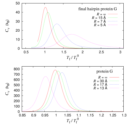
Figure 5: Specific heat $C_{V}=\frac{1}{k_{B}T^{2}}\frac{\partial^{2}\ln Z}{\partial\beta^{2}}$ as a function of the temperature at various confinement radius $R$ for protein G and its final hairpin.

A fit to (6) of unfolding temperatures as a function of $R$ (figure 6) yielded exponents $\gamma$ reported in table 2. All values are in between $1.50$ ($3$–helix bundle) and $2.35$ (final hairpin of protein G). Remarkably, in this range we find also the theoretical values of $\gamma$ for an excluded volume chain confined in a slit or in a cylinder ($\gamma=5/3$) and for a gaussian chain in a slit, a cylinder or a sphere ($\gamma=2$). Furthermore, a more careful analysis of data in figure 6 suggested us to fit, in the case of the $\beta$–hairpins, also in a more limited range of $R$ values going from $L_{\mbox{\scriptsize{U }\footnotesize{eff.}}}/2$ to $L_{\mbox{\footnotesize{max}}}$ (figure 7). In this very low confinement regime $\gamma=1.72$ for the ideal hairpin and $\gamma=1.6$ for the final hairpin of protein G.

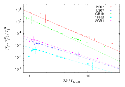
Figure 6: Shift in unfolding temperature as a function of confining cage radius $R$. Fits to (6) in ranges reported in table 2. The vertical lines represent the ranges spanned by fits.

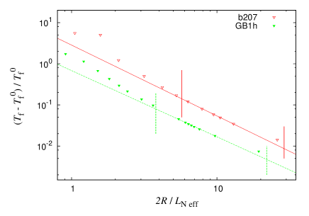
Figure 7: Shift in unfolding temperature as a function of confining cage radius $R$ for ‘b207’ and ‘GB1h’. Fits to (6) in ranges $L_{\mbox{\scriptsize{U }\footnotesize{eff.}}}/2$ to $L_{\mbox{\footnotesize{max}}}$. The vertical lines represent the ranges spanned by fits.

3.2 Kinetics

The folding kinetics have been studied by Monte Carlo (MC) simulations in which a $2$–components ternary variable $(m_{k},s_{k})$ have been associated to each residue $k$. If $m_{k}=1$, $s_{k}=0$ while if $m_{k}=0$, $s_{k}=\sigma_{kj}=\pm 1$ is the direction of the native stretch from the $k$–th to the $j$-th residue. A single MC step consists in choosing a residue $k$ with uniform probability among the $N$ residues and changing $(m_{k},s_{k})$ variable with equal probability to any of its other two states. This move is alternated with a $0.1$ Å  translation of the entire protein to the left or to the right with equal probability. Few remarks are necessary: suppose to have a native stretch from the $i$–th to the $j$-th residue and to transform the variable $(m_{k},s_{k})$, $i<k<j$, from $(1,0)$ to $(0,s_{k}=\pm 1)$. The direction of the new native stretch from the $k$–th to the $j$-th residue will be determined by $s_{k}$ while the new native stretch from $i$ to $k$ will inherit the direction of the old one from $i$ to $j$. If instead we move the state of $k$–th residue from $(0,\pm 1)$ to $(1,0)$, two native stretches merge into one with direction equal to the direction of the first old native stretch. At each MC step confinement requirements must be checked.

Changes in folding rates have been estimated [18] from Kramers kinetics, $k_{\mbox{\footnotesize{f}}}\propto D\exp(-\Delta G_{\mbox{\scriptsize{U}}}^{\mbox{\scriptsize{barrier}}}/k_{B}T)$, where $\Delta G_{\mbox{\scriptsize{U}}}^{\mbox{\scriptsize{barrier}}}$ is the free energy difference between the transition state and the unfolded state and $D$ is a diffusion coefficient. Because the unfolded state is destabilized by confinement, the free energy barrier dividing the unfolded from the native state is smaller. Assuming that the free energy of the latter and the diffusion constant are not affected by confinement and that the free energy of the unfolded state grows by a term $\sim T(R/L_{0})^{-\gamma}$ [20, 21] leads to the scaling law:

$$\ln\left(\frac{k_{\mbox{\footnotesize{f}}}}{k_{\mbox{\footnotesize{f}}}^{0}}\right)\propto\left(\frac{2R}{L_{\mbox{\scriptsize{N }\footnotesize{eff.}}}}\right)^{-\gamma}$$ (7)

We determined folding rates as the inverse of mean first passage times by using $10^{4}$ folding trajectories. First passage time is defined as the time at which, starting from a random unfolded configuration, the weighted fraction of native contacts ($Q=\sum_{i=1}^{N-1}\sum_{j=i+1}^{N}\varepsilon_{ij}\Delta_{ij}\prod_{k=i}^{j}m_{k}/\sum_{i=1}^{N-1}\sum_{j=i+1}^{N}\varepsilon_{ij}\Delta_{ij}$) catches up with the threshold $0.9$, which ensures the protein has reached the folded state and has not got stuck in some intermediate. Temperature has been set to $0.9\,T_{\mbox{\footnotesize{f}}}^{0}$.

Table 3: Values of $R$ for which the folding rate reaches its maximum $k_{\mbox{\footnotesize{f}}}^{\mbox{\scriptsize{max}}}$ at $T=0.9\,T_{\mbox{\footnotesize{f}}}^{0}$ and the extent of enhancement. Values of $\gamma$ from fits to (7) in the reported ranges.

• 	b207	b307	GB1h	1PRB	2GB1
  $R_{\mbox{\scriptsize{I}}}^{\mbox{\footnotesize{kin}}}$ (Å)	$19$	$23$	$12$	$19$	$18$
  $k_{\mbox{\footnotesize{f}}}^{\mbox{\scriptsize{max}}}$	$1.13\,k_{\mbox{\footnotesize{f}}}^{0}$	$1.13\,k_{\mbox{\footnotesize{f}}}^{0}$	$1.46\,k_{\mbox{\footnotesize{f}}}^{0}$	$1.50\,k_{\mbox{\footnotesize{f}}}^{0}$	$2.35\,k_{\mbox{\footnotesize{f}}}^{0}$
  $\gamma$	$1.42\pm 0.20$	$1.53\pm 0.33$	$1.54\pm 0.11$	$1.71\pm 0.08$	$1.67\pm 0.07$
  fit range (Å)	$[19,50]$	$[23,76]$	$[14,64]$	$[22,201]$	$[20,212]$

When decreasing $R$, folding is accelerated until a certain size $R_{\mbox{\scriptsize{I}}}^{\mbox{\footnotesize{kin}}}$ is reached, then folding rates start to decrease. Table 3 reports $R_{\mbox{\scriptsize{I}}}^{\mbox{\footnotesize{kin}}}$ values and the maximum extent of folding rates enhacement. For the $\beta$–hairpins, the drastic difference between $R_{\mbox{\scriptsize{I}}}^{\mbox{\footnotesize{kin}}}$ and $R_{\mbox{\scriptsize{I}}}^{\mbox{\footnotesize{eq}}}$ is likely due to the fact that for very small confining cages, even if the native state is not compromised, the structure is squeezed so much that chain reconfigurations towards the folded state become difficult. The same reason should explain the small differences between $R_{\mbox{\scriptsize{I}}}^{\mbox{\footnotesize{kin}}}$ and $R_{\mbox{\scriptsize{I}}}^{\mbox{\footnotesize{eq}}}$ of other structures.

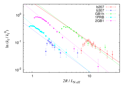
Figure 8: Shift in folding rates at $T=0.9\,T_{\mbox{\footnotesize{f}}}^{0}$ as a function of confining cage radius $R$. Fits to (7) in ranges reported in table 3.

Table 3 also reports the $\gamma$ values obtained through a fit to (7) while figure 8 shows the folding rates behavior together with fit lines. If for the two hairpins we considered the very–low confinement regime, exponents $\gamma$ relative to folding rates are comparable with their equilibrium counterparts.

4 Conclusions

We have investigated the effects of confinement on protein thermal stability and folding kinetics using a simple Ising–like model that we have contributed to develop and validate in recent years and now properly modified to include confinement of a polypeptide chain into a slit. To study thermal stability we have made use of the property of the model to be exactly solvable at equilibrium, while to study folding rates behavior we have resorted to Monte Carlo simulations. Notwithstanding the simplicity of the model and its unidimensionality, we obtained results which follow the general trend of previous experimental studies [9, 10, 11, 41] and simulations [16, 17, 18]: provided the native state is compact, when reducing the space available to a given protein, both unfolding temperature $T_{\mbox{\footnotesize{f}}}$ and folding rate $k_{\mbox{\footnotesize{f}}}$ grow until a certain confinement size which depends on the protein. If the confinement size is further decreased, unfolding temperatures and folding rates decrease. Furthermore, our results also support the theoretical prediction [13, 17, 18] that enhancement depends on the confinement size $R$ by the scaling law $\Delta T_{\mbox{\footnotesize{f}}}\sim\Delta\ln k_{\mbox{\footnotesize{f}}}\sim R^{-\gamma}$.

Among the six different protein structures studied in this work, one, a $10$–residues ideal $\alpha$–helix, does not show any enhancement of folding temperature and rate because its native state cannot be considered compact if compared to the average unfolded state. For the other five structures we found that exponents $\gamma$ lie in between the upper and lower values of $2.35$ and $1.42$ and that those obtained for unfolding temperatures from exact solutions at equilibrium are consistent with those obtained for folding rates enhancement by Monte Carlo simulations.

Theoretical values of $\gamma$ ($\gamma=5/3$ for a chain with excluded volume confined into a slit or a cylinder and $\gamma=2$ for a gaussian chain into a slit, a cylinder or a sphere) are not directly comparable to the results of our model, which differs from these theories both for the geometry (our chain is neither self-avoiding nor gaussian) and for the presence of specific interactions, which are neglected by these theories. Nevertheless, our results, both from thermodynamics and kinetics, for $\gamma$, are in the same range as the theoretical ones.

Furthermore, for a $3$–helix bundle and for protein G, our results are consistent with those obtained through a more realistic model by Best and Mittal [18] for confinement of the same proteins into a slit: $\gamma$ values are consistent and also the maximum enhancement extents of folding temperatures and folding rates are in good accordance. The two model also agree in the fact that protein G is more affected by confinement but there is no accordance on the confinement radius at which the $3$–helix bundle reaches its maximum folding temperature and its maximum folding rate.

References

References

- [1] Ellis R.J. Macromolecular crowding: obvious but underappreciated. Trends Biochem. Sci., 26:597–604, 2001.
- [2] Minton A.P. Influence of excluded volume upon macromolecular structure and associations in ‘crowded’ media. Curr. Opin. Biotechnol., 8:65–69, 1997.
- [3] Minton A.P. Implication of macromolecular crowding for protein assembly. Curr. Opin. Struct. Biol., 10:34–39, 2000.
- [4] Ellis R.J. Macromolecular crowding: an important but neglected aspect of the intracellular environment. Curr. Opin. Struct. Biol., 11:114–119, 2001.
- [5] Zimmerman S.B. and Trach S.O. Estimation of macromolecule concentrations and excluded volume effects for the cytoplasm of escherichia coli. J. Mol. Biol., 222:599–620, 1991.
- [6] Cheung M.S., Klimov D.K., and Thirumalai D. Molecular crowding enhances native state stability and refolding rates of globular proteins. Proc. Natl. Acad. Sci. USA, 102:4753–58, 2005.
- [7] Gershenson A. and Gierasch L.M. Protein folding in the cell: challenges and progress. Curr. Opin. Struct. Biol., 21:32–41, 2011.
- [8] Eggers D. and Valentine J.S. Molecular confinement influences protein structure and enhances thermal protein stability. Protein Sci., 10:250–261, 2001.
- [9] Campanini B., Bologna S., Cannone F., Chirico G., Mozzarelli A., and Bettati S. Unfolding of green fluorescent protein mut2 in wet nanoporous silica gels. Protein Sci., 14:1125–33, 2005.
- [10] Ravindra R., Zhao S., Gies H., and Winter R. Protein encapsulation in mesoporous silicate: The effects of confinement on protein stability, hydration, and volumetric properties. J. Am. Chem. Soc., 126:12224–225, 2004.
- [11] Bolis D., Politou A.S., Kelly G., Pastore A., and Temussi P.A. Protein stability in nanocages: A novel approach for influencing protein stability by molecular confinement. J. Mol. Biol., 336:203–212, 2004.
- [12] Hong J. and Gierasch L.M. Macromolecular crowding remodels the energy landscape of a protein by favoring a more compact unfolded state. J. Am. Chem. Soc., 132:10445–10452, 2010.
- [13] Zhou HX. Protein folding and binding in confined spaces and in crowded solutions. J. Mol. Recognit., 17:368–375, 2004.
- [14] Zhou HX. Protein folding in confined and crowded environments. Arch. Biochem. Biophys., 469:76–82, 2008.
- [15] Thirumalai D., Klimov D.K., and Lorimer G.H. Caging helps proteins fold. Proc. Natl. Acad. Sci. USA, 100:11195–197, 2003.
- [16] Klimov D.K., Newfield D., and Thirumalai D. Simulations of -hairpin folding confined to spherical pores using distributed computing. Proc. Natl. Acad. Sci. USA, 99:8019–24, 2002.
- [17] Takagi F., Koga N., and Takada S. How protein thermodynamics and folding mechanisms are altered by chaperonin cage: Molecular simulations. Proc. Natl. Acad. Sci. USA, 100:11367–372, 2003.
- [18] Mittal J. and Best R.B. Thermodynamics and kinetics of protein folding under confinement. Proc. Natl. Acad. Sci. USA, 105:20233–238, 2008.
- [19] Hayer-Hartl M. and Minton A.P. A simple semiempirical model for the effect of molecular confinement upon the rate of protein folding. Biochemistry, 45:13356–360, 2006.
- [20] de Gennes P.G. Scaling Conceps in Polymer Physics. Cornell University Press, 1979.
- [21] Sakaue T. and Raphaël E. Polymer chains in confined spaces and flow-injection problems: Some remarks. Macromolecules, 39:2621–28, 2006.
- [22] Cordeiro C.E., Molisana M., and Thirumalai D. Shape of a confined polymer chains. J. Phys. II France, 7:433–447, 1997.
- [23] Wako H. and Saitô N. Statistical mechanical theory of the protein conformation. i. general considerations and the application to homopolymers. J. Phys. Soc. Jpn, 44:1931–39, 1978.
- [24] H. Wako and N. Saitô. Statistical mechanical theory of the protein conformation. ii. folding pathway for protein. J. Phys. Soc. Jpn, 44:1939–45, 1978.
- [25] Muñoz V., Thompson P.A., Hofrichter J., and Eaton W.A. Folding dynamics and mechanism of –hairpin formation. Nature, 390:196–199, 1997.
- [26] Muñoz V., Henry E.R., Hofrichter J., and Eaton W.A. A statistical mechanical model for –hairpin kinetics. Proc. Natl. Acad. Sci. USA, 95:5872–79, 1998.
- [27] Muñoz V. and Eaton W.A. A simple model for calculating the kinetics of protein folding from three–dimensional structures. Proc. Natl. Acad. Sci. USA, 96:11311–316, 1999.
- [28] Bruscolini P. and Pelizzola A. Exact solution of the Muñoz–Eaton model for protein folding. Phys. Rev. Lett., 88:258101, 2002.
- [29] Pelizzola A. Exactness of the cluster variation method and factorization of the equilibrium probability for the Wako–Saitô–Muñoz–Eaton model of protein folding. J. Stat. Mech.: Theory Exp., page P11010 (14), 2005.
- [30] Zamparo M. and Pelizzola A. Kinetics of the Wako–Saitô–Muñoz–Eaton model of protein folding. Phys. Rev. Lett., 97:068106, 2006.
- [31] Zamparo M. and Pelizzola A. Rigorous results on the local equilibrium kinetics of a protein folding model. J. Stat. Mech.: Theory Exp., page P12009 (22), 2006.
- [32] Bruscolini P., Pelizzola A., and Zamparo M. Downhill versus two–state protein folding in a statistical mechanical model. J. Chem. Phys., 126:215103 (8), 2007.
- [33] Bruscolini P., Pelizzola A., and Zamparo M. Rate determining factors in protein model structures. Phys. Rev. Lett., 99:038103, 2007.
- [34] Imparato A., Pelizzola A., and Zamparo M. Ising–like model for protein mechanical unfolding. Phys. Rev. Lett., 98:148102, 2007.
- [35] Imparato A., Pelizzola A., and Zamparo M. Protein mechanical unfolding: A model with binary variables. J. Chem. Phys., 127:145105 (11), 2007.
- [36] Imparato A. and Pelizzola A. Mechanical unfolding and refolding pathways of ubiquitin. Phys. Rev. Lett., 100:158104, 2008.
- [37] Imparato A., Pelizzola A., and Zamparo M. Equilibrium properties and force–driven unfolding pathways of RNA molecules. Phys. Rev. Lett., 103:188102, 2009.
- [38] Caraglio M., Imparato A., and Pelizzola A. Pathways of mechanical unfolding of FnIII10: Low force intermediates. J. Chem. Phys., 133:065101 (9), 2010.
- [39] Caraglio M., Imparato A., and Pelizzola A. Direction dependent mechanical unfolding and green fluorescent protein as a force sensor. Phys. Rev. E, 2011. in press.
- [40] Faccin M., Bruscolini P., and Pelizzola A. Analysis of the equilibrium and kinetics of the ankyrin repeat protein myotrophin. J. Chem. Phys., 134:075102 (11), 2011.
- [41] Tang Y-C., Chang H-C., Roeben A., Wischnewski D., Wischnewski N., Kerner M.J., Hartl F.U., and Hayer-Hartl M. Structural features of the groEL–groES Nano–Cage required for rapid folding of encapsulated protein. Cell, 125:903–914, 2006.