JIMWLK evolution in the Gaussian approximation

Abstract

We demonstrate that the Balitsky–JIMWLK equations describing the high–energy evolution of the $n$–point functions of the Wilson lines (the QCD scattering amplitudes in the eikonal approximation) admit a controlled mean field approximation of the Gaussian type, for any value of the number of colors $N_{c}$. This approximation is strictly correct in the weak scattering regime at relatively large transverse momenta, where it reproduces the BFKL dynamics, and in the strong scattering regime deeply at saturation, where it properly describes the evolution of the scattering amplitudes towards the respective black disk limits. The approximation scheme is fully specified by giving the 2–point function (the $S$–matrix for a color dipole), which in turn can be related to the solution to the Balitsky–Kovchegov equation, including at finite $N_{c}$. Any higher $n$–point function with $n\geq 4$ can be computed in terms of the dipole $S$–matrix by solving a closed system of evolution equations (a simplified version of the respective Balitsky–JIMWLK equations) which are local in the transverse coordinates. For simple configurations of the projectile in the transverse plane, our new results for the 4–point and the 6–point functions coincide with the high–energy extrapolations of the respective results in the McLerran–Venugopalan model. One cornerstone of our construction is a symmetry property of the JIMWLK evolution, that we notice here for the first time: the fact that, with increasing energy, a hadron is expanding its longitudinal support symmetrically around the light–cone. This corresponds to invariance under time reversal for the scattering amplitudes.

1 Introduction

The final state of an ultrarelativistic hadron–hadron collision, as currently explored at RHIC and the LHC, is characterized by an extreme complexity in terms of the number and the distribution of the produced particles. The study of multiparticle correlations represents an essential tool for organizing this complexity and extracting physical information out of it. In particular, a recent measurement at RHIC of di–hadron correlations in deuteron–gold collisions Braidot:2011zj revealed an interesting phenomenon — the azimuthal correlations are rapidly suppressed when increasing the rapidity towards the fragmentation region of the deuteron —, which is qualitatively JalilianMarian:2004da ; Nikolaev:2005dd ; Baier:2005dv ; Marquet:2007vb and even semi–quantitatively Albacete:2010pg ; Stasto:2011ru consistent with the physical picture of gluon saturation in the nuclear wavefunction. For this interpretation to be firmly established, one needs a more precise understanding of the multi–particle correlations in the high–energy scattering and, in particular, of their evolution with increasing rapidity. This triggered new theoretical studies Dumitru:2010ak ; Dominguez:2011wm ; Dominguez:2011gc ; Dumitru:2011vk ; Iancu:2011ns of many–body correlations in the color glass condensate (CGC), which is the QCD effective theory for high–energy evolution and gluon saturation, to leading logarithmic accuracy at least.

The central ingredient in the CGC theory is the JIMWLK (Jalilian-Marian, Iancu, McLerran, Weigert, Leonidov, Kovner) equation JalilianMarian:1997jx ; JalilianMarian:1997gr ; JalilianMarian:1997dw ; Kovner:2000pt ; Weigert:2000gi ; Iancu:2000hn ; Iancu:2001ad ; Ferreiro:2001qy , a functional renormalization group equation of the Fokker–Planck type which describes the non–linear evolution of the gluon distribution in the hadron wavefunction with increasing rapidity, or decreasing the gluon longitudinal momentum fraction $x$. When applied to an asymmetric, ‘dilute–dense’, scattering (like a $pA$ collision), the JIMWLK evolution can be equivalently reformulated as an infinite hierarchy of ordinary evolution equations, originally derived by Balitsky Balitsky:1995ub , which refer to gauge–invariant correlations built with products of Wilson lines. A ‘Wilson line’ is a path–ordered exponential of the color field in the target. It describes the scattering between a parton from the projectile (the proton) and the dense gluonic system in the target (the nucleus), in the eikonal approximation. Via the optical theorem, the $n$–point functions of the Wilson lines can be related to cross–sections for particle production in $pA$ collisions. For instance, the single–inclusive quark (or gluon) production is related to the $S$–matrix of a ‘color dipole’ (the 2–point function of the Wilson lines). Similarly, the production of a pair of partons with similar rapidities is related to the ‘color quadrupole’ (the 4–point function). The suppression of azimuthal di–hadron correlations in d+Au collisions at RHIC Braidot:2011zj occurs in the right range of transverse momenta, of the order of the nuclear saturation momentum $Q_{s}\sim 1$ GeV, to be interpreted as a result of gluon saturation and multiple interactions in the scattering of the quadrupole. Such non–linear phenomena are mean field effects, which are likely to be correctly described by the JIMWLK evolution, although the latter is known to miss another important class of correlations — those associated with gluon number fluctuations in the dilute regime, or ‘Pomeron loops’ Iancu:2004es ; Iancu:2004iy ; Mueller:2005ut ; Iancu:2005nj ; Kovner:2005nq .

Motivated by the above considerations, there were several recent studies of the quadrupole evolution in the framework of the Balitsky–JIMWLK equations Dominguez:2011gc ; Dumitru:2011vk ; Iancu:2011ns . The results in Ref. Dumitru:2011vk appeared as particularly intriguing. In that paper, one has numerically solved the JIMWLK equation by using its representation as a functional Langevin process Blaizot:2002xy and used the results to evaluate the quadrupole $S$–matrix for different rapidities and for special configurations of the 4 external points in the transverse plane. Remarkably, the results thus obtained show a very good agreement with the heuristic extrapolation to high energy of the corresponding results in the McLerran–Venugopalan (MV) model McLerran:1993ni ; McLerran:1993ka . We recall that the MV model refers to a large nucleus ($A\gg 1$) at not too high energy (where the effects of the evolution are still negligible) and that in this model the CGC weight function is taken to be a Gaussian: the only non–trivial correlation of the color fields in the nucleus is their 2–point function, the ‘unintegrated gluon distribution’. The ‘high–energy extrapolation’ alluded to above refers to using the MV expression for the quadrupole $S$–matrix in terms of the dipole $S$–matrix JalilianMarian:2004da ; Dominguez:2011wm , but with the latter taken from the numerical solution to the JIMWLK equation at the rapidity of interest.

Such extrapolations have often been used for phenomenological studies Kovner:2001vi ; Blaizot:2004wv ; JalilianMarian:2004da ; Marquet:2010cf ; Kuokkanen:2011je ; Dominguez:2011wm ; Muller:2011bb , but their justification from the viewpoint of the high–energy evolution remained obscure. A Gaussian Ansatz has also been used for mean field studies of the Balitsky–JIMWLK evolution Iancu:2001md ; Iancu:2002xk ; Iancu:2002aq ; Kovchegov:2008mk . But these previous studies have not convincingly addressed the issue of the validity of the Gaussian approximation — in particular, they did not justify its suitability for describing higher $n$–point functions, such as the quadrupole. (The only, qualitative, attempt in that sense is the ‘random phase approximation’ proposed in Ref. Iancu:2001md ; see the discussion in Sect. 3.4 below.) In principle, there is no contradiction between having a Gaussian weight function for the target field and still generating non–trivial correlations in the scattering of many–body projectiles: indeed, the scattering amplitudes are built with Wilson lines, which are non–linear in the target field to all orders. But within the context of the JIMWLK evolution, such Gaussian approximations seem to be prohibited by the highly non–linear structure of the evolution equation, which is the mathematical expression of gluon saturation.

In spite of this theoretical prejudice, the numerical results in Ref. Dumitru:2011vk suggest that a Gaussian approximation to the JIMWLK evolution may nevertheless work. Another piece of evidence in that sense emerges from the recent analytic study in Ref. Iancu:2011ns . There, we have constructed an approximate version of the Balitsky–JIMWLK hierarchy which is simple enough to allow for explicit solutions. Then we have showed that, for the special configurations of the quadrupole considered in Ref. Dumitru:2011vk , these approximate solutions coincide with the respective predictions of the MV model extrapolated to high energy. But in that context too, the similarity with the MV model appears as merely an ‘accident’, with no deep motivation: the simplified hierarchy proposed in Ref. Iancu:2011ns is generated by the ‘virtual’ piece of the JIMWLK Hamiltonian, which is non–linear in the target field and therefore seems incompatible with a Gaussian approximation. Moreover, the approximations in Ref. Iancu:2011ns have been justified only in the limit where the number of colors $N_{c}$ is large (formally, $N_{c}\to\infty$). This does not explain the observation in Ref. Dumitru:2011vk that the numerical solutions to the JIMWLK evolution for $N_{c}=3$ are better reproduced by the finite–$N_{c}$ version of the MV model (with $N_{c}=3$, of course) than by its large–$N_{c}$ limit.

Our purpose in the present analysis is to clarify such ‘coincidences’ and ‘apparent contradictions’ by resolving the aforementioned tensions between the simplified hierarchy proposed in Ref. Iancu:2011ns , the Gaussian approximation, and the large–$N_{c}$ limit. The results that we shall obtain can be summarized as follows. We shall demonstrate that the JIMWLK equation admits indeed an approximate Gaussian solution for the CGC weight function, that this solution is unique within the limits of its accuracy, and that it is tantamount to a simplified system of evolution equations, which are linear (while being consistent with unitarity) and local in the transverse coordinates. In the limit where $N_{c}\to\infty$, these new equations reduce to those previously proposed in Ref. Iancu:2011ns . The ultimate outcome of our analysis is a global approximation to the Balitsky–JIMWLK hierarchy, which is valid for any $N_{c}$ and allows one to construct explicit, analytic, solutions for all the $n$–point functions of the Wilson lines. These approximate solutions are strictly correct in the limiting regimes at very large ($k_{\perp}\gg Q_{s}(Y)$) and, respectively, very small ($k_{\perp}\ll Q_{s}(Y)$) transverse momenta, and provide a smooth (infinitely differentiable) interpolation between these limits. Here, $Q_{s}(Y)$ denotes the saturation momentum in the target at a rapidity $Y$ equal with the rapidity separation between the target and the projectile.

To describe our results in more detail, let us first explain the distinction between ‘real’ and ‘virtual’ terms in the Balitsky–JIMWLK equations. The ‘real’ terms describe the evolution of the projectile via the emission of small–$x$ gluons, whereas the ‘virtual’ terms express the probability for the projectile not to evolve, i.e. not to radiate such (small–$x$) gluons. The ‘virtual’ terms dominate the evolution in the approach towards the unitarity (or ‘black disk’) limit, since in that regime the scattering is strong and the projectile has more chances to survive unscattered if it remains ‘simple’ — i.e., if it does not evolve by emitting more gluons. By the same token, the ‘virtual’ terms control the evolution of the many–body correlations which, within the context of JIMWLK, are built exclusively via non–linear effects (multiple scattering and gluon recombination) in the regime of strong scattering. More precisely, the ‘real’ terms are important for that process too — they include the non–linear effects responsible for unitarity and saturation —, but deeply at saturation their role becomes very simple: they merely prohibit the emission of new gluons with low transverse momenta $k_{\perp}\lesssim Q_{s}(Y)$. Thus, one can follow the evolution of correlations at saturation by keeping only the ‘virtual’ terms in the Balitsky–JIMWLK equations, but supplementing them with a phase–space cutoff which expresses the effect of the ‘real’ terms. (This is strictly correct in a ‘leading–logarithmic approximation’ to be detailed in Sect. 3.4.) Moreover, since the simplified equations thus obtained are linear, they can be extended to also cover the BFKL evolution in the weak scattering regime at $k_{\perp}\gg Q_{s}(Y)$. Indeed, in that regime and to the accuracy of interest, the $n$–point functions of the Wilson lines reduce to linear combinations of the dipole scattering amplitude, with the latter obeying the BFKL equation. The BFKL dynamics involves both ‘real’ and ‘virtual’ terms, but it can be effectively taken into account by tuning the kernel in the ‘virtual’ terms — namely, by requiring this kernel to approach the solution to the BFKL equation at large $k_{\perp}$.

The above considerations, to be substantiated by the subsequent analysis, explain why it is possible to approximate the Balitsky–JIMWLK equations by simpler equations which are linear and whose overall structure is inherited from the ‘virtual’ terms in the original equations. Similar considerations have underlined our previous construction in Ref. Iancu:2011ns , but their generalization to finite $N_{c}$ (that we shall provide in this paper) turns out to be highly non–trivial.

Another subtle aspect of our present analysis is the recognition of the fact that the simplified equations that we shall propose (for either finite or infinite $N_{c}$) correspond to a Gaussian approximation for the CGC weight function. A priori, the association of a linear system of equations with a Gaussian approximation may look natural, but in the present case this is complicated by the fact that, as alluded to before, the ‘virtual’ piece of the JIMWLK Hamiltonian is non–linear in the target field to all orders. Such a non–linear structure seems to preclude any Gaussian solution. The resolution of this mathematical puzzle turns out to be interesting on physical grounds, as it sheds new light on the physical picture of the JIMWLK evolution. Namely, we shall show that the Wilson lines within the ‘virtual’ Hamiltonian do not represent genuine non–linear effects associated with saturation, rather they express the physical fact that, with increasing energy, the longitudinal support of the target expands symmetrically around the light–cone. That is, in contrast to a widespread opinion in the literature (see e.g. Iancu:2002xk ; Iancu:2002aq ; Blaizot:2002xy ; Iancu:2003xm ; Kovchegov:2008mk ), which was based on a misinterpretation of the mathematical structure of the JIMWLK equation, the gluon distribution in the target expands simultaneously towards larger and respectively smaller values of $x^{-}$, in such a way to remain symmetric around $x^{-}=0$. (We assume the target to propagate along the positive $x^{3}$ axis at nearly the speed of light and we define $x^{-}=(x^{0}-x^{3})/\sqrt{2}$.) In turn, this symmetry has physical consequences for the multi–partonic scattering amplitudes: it implies that the $n$–point functions of the Wilson lines with $n\geq 4$ obey a special permutation symmetry — the mirror symmetry — which expresses their invariance under time reversal.

To summarize, a Gaussian weight function which is symmetric in $x^{-}$ and whose kernel is energy–dependent and interpolates between the solution to the BFKL equation at high transverse momenta $k_{\perp}\gg Q_{s}$ and the JIMWLK (or ‘dipole’) kernel at low momenta $k_{\perp}\ll Q_{s}$, provides a reasonable approximation to the JIMWLK equation, which is strictly correct in the limiting regimes alluded to above (for any value of $N_{c}$). Within its limits of validity, this approximation is essentially unique: different constructions for the kernel can differ from each other only in the transition region around saturation, which is anyway not under control within the present approximation.

In practice, it is convenient to trade this kernel for the dipole $S$–matrix, which in turn can be obtained either as the solution to the Balitsky–Kovchegov (BK) equation Balitsky:1995ub ; Kovchegov:1999yj , or by solving a self–consistency condition similar to that in Ref. Iancu:2002xk . (The differences between these two expressions for the kernel should be viewed as an indicator of the stability of the approximation scheme.) Then the $n$–point functions with $n\geq 4$ (quadrupole, sextupole etc) can be determined in terms of the 2–point function (the dipole $S$–matrix) by solving the evolution equations associated with the Gaussian weight function. These equations become particularly simple at large $N_{c}$, where they reduce to the equations proposed in Ref. Iancu:2011ns and can be explicitly solved for arbitrary configurations of the $n$ external points in the transverse plane.

For finite $N_{c}$ and for generic configurations, the equations are more complicated, as they couple the evolution of the various $n$–point functions with the same value of $n$. (For instance, the quadrupole mixes under the evolution with a system of two dipoles.) Yet, explicit solutions can be obtained under the simplifying assumption that the kernel of the Gaussian is a separable function of the rapidity and the transverse coordinates (plus an arbitrary function of $Y$; see Sect. 4.2 for details). This is certainly not the case for the actual kernel (say, as given by the solution to the BK equation), but it is a good piecewise approximation to it and it is furthermore true for the MV model, that we shall take as our initial condition at low energy. So, not surprisingly, the expressions for the $n$–point functions that we shall obtain within this scenario are formally similar to the respective predictions of the MV model. One can reverse this last argument as follows: given that the Gaussian weight function is a good, piecewise approximation to the JIMWLK evolution, as we shall demonstrate, and that the kernel of this Gaussian can be taken to be separable within the relevant kinematical regimes, we expect the predictions of this approximation to be very close to those of the MV model extrapolated to high energy.

For special configurations which are highly symmetric, exact solutions can be obtained at finite $N_{c}$ even without assuming separability. We shall study various examples of this type for the 4–point function and the 6–point function, and thus find some surprising factorization properties, that would be interesting to test against numerical solutions to the JIMWLK equation. For one particular configuration of the 6–point function, the exact numerical result is already known Dumitru:2011vk and our respective analytic solution appears to agree with it quite well.

2 The Balitsky–JIMWLK evolution equations

In this section, we shall briefly review the general formulation of the JIMWLK evolution and then use the evolution equations satisfied by the dipole and the quadrupole $S$–matrices in order to illustrate various properties of the evolution, which are important for what follows: the role and origin of the ‘real’ and ‘virtual’ terms, the factorization of multi–trace observables at large $N_{c}$, and, especially, the symmetric expansion of the longitudinal support of the target and the ensuing, ‘mirror’, symmetry of the $n$–point functions with $n\geq 4$.

2.1 JIMWLK evolution: a brief reminder

The color glass condensate is an effective theory for the small–$x$ part of the wavefunction of an energetic hadron: the gluons carrying a small fraction $x\ll 1$ of the hadron’s longitudinal momentum are described as a random distribution of classical color fields generated by sources with larger momentum fractions $x^{\prime}\gg x$. Given the high–energy kinematics, in particular the fact that the distribution of the color sources is ‘frozen’ by Lorentz time dilation, this color field can be chosen (in a suitable gauge) to have a single non–zero component, namely $A^{\mu}_{a}(x)=\delta^{\mu+}\alpha_{a}(x^{-},\bm{x})$ for a hadron moving along the positive $z$ axis (a ‘right mover’). All the correlations of this field are encoded into a functional probability distribution, the ‘CGC weight function’ $W_{Y}[\alpha]$, which contains information about the evolution of the color sources with increasing ‘rapidity’ $Y\equiv\ln(1/x)$, from some initial value $Y_{0}$ up to the value $Y$ of interest. In the high energy regime where $\alpha_{s}(Y-Y_{0})\gtrsim 1$ and to leading logarithmic accuracy with respect to the large logarithm $Y-Y_{0}=\ln(x_{0}/x)$, this evolution is described by a functional renormalization group equation for $W_{Y}[\alpha]$, known as the JIMWLK equation. The latter can be given a Hamiltonian form,

$$\frac{\partial}{\partial Y}W_{Y}[\alpha]=HW_{Y}[\alpha]\,,$$ (2.1)

where $H$ is the JIMWLK Hamiltonian — a second–order, functional differential operator, whose most convenient form for the present purposes is that given in Hatta:2005as and reads

$$H=-\frac{1}{16\pi^{3}}\int_{\bm{u}\bm{v}\bm{z}}\mathcal{M}_{\bm{u}\bm{v}\bm{z}}\left(1+\widetilde{V}^{\dagger}_{\bm{u}}\widetilde{V}_{\bm{v}}-\widetilde{V}^{\dagger}_{\bm{u}}\widetilde{V}_{\bm{z}}-\widetilde{V}^{\dagger}_{\bm{z}}\widetilde{V}_{\bm{v}}\right)^{ab}\frac{\delta}{\delta\alpha_{\bm{u}}^{a}}\frac{\delta}{\delta\alpha_{\bm{v}}^{b}},$$ (2.2)

where we use the notation $\int_{\bm{u}\dots}\equiv\int{\rm d}^{2}\bm{u}\dots$ to simplify writing, $\mathcal{M}$ is the ‘dipole kernel’,

$$\mathcal{M}_{\bm{u}\bm{v}\bm{z}}\,\equiv\,\frac{(\bm{u}-\bm{v})^{2}}{(\bm{u}-\bm{z})^{2}(\bm{z}-\bm{v})^{2}}\,,$$ (2.3)

and $\widetilde{V}^{\dagger}$ and $\widetilde{V}$ are Wilson lines in the adjoint representation:

$$\widetilde{V}^{\dagger}_{\bm{x}}\,\equiv\,{\mbox{P}}\exp\left[{\rm i}g\int{\rm d}x^{-}\alpha_{a}(x^{-},\bm{x})T^{a}\right],$$ (2.4)

with P denoting path–ordering in $x^{-}$. The above form of the Hamiltonian is valid only when acting on gauge–invariant functionals of $\alpha_{a}$, which will always be the case throughout our analysis. In fact, the observables of interest are gauge–invariant products of Wilson lines (see below).

The functional derivatives in Eq. (2.2) are understood to act at the largest value of $x^{-}$, that is, at the upper end point of path–ordered exponentials like that in Eq. (2.4) (see e.g. Eq. (2.11)). These derivatives do not commute with each other, but their commutator is proportional to $\delta_{\bm{u}\bm{v}}$ (cf. Eq. (2.27)) and thus vanishes when multiplied by $\mathcal{M}_{\bm{u}\bm{v}\bm{z}}$; hence, there is no ambiguity concerning the ordering of the functional derivatives in Eq. (2.2). One can also notice that the last two terms in the JIMWLK Hamiltonian, i.e. those proportional to $\widetilde{V}^{\dagger}_{\bm{u}}\widetilde{V}_{\bm{z}}$ and to $\widetilde{V}^{\dagger}_{\bm{z}}\widetilde{V}_{\bm{v}}$ respectively, are in fact identical to each other, as it can be checked by exchanging $\bm{u}\leftrightarrow\bm{v}$ and $a\leftrightarrow b$ and by using the property $\widetilde{V}^{\dagger\,ac}_{\bm{z}}=\widetilde{V}^{ca}_{\bm{z}}$ for color matrices in the adjoint representation. To fully specify the problem, one also needs an initial condition for Eq. (2.1) at $Y=Y_{0}$; at least for a sufficiently large nucleus, this initial condition is provided by the McLerran–Venugopalan (MV) model McLerran:1993ni ; McLerran:1993ka (see Sect. 3.2 below).

Physical observables, like scattering amplitudes for external projectiles, are represented by gauge invariant operators $\hat{\mathcal{O}}[\alpha]$ built with the field $\alpha_{a}$, whose target expectation values are computed via functional averaging with the CGC weight function:

$$\langle\hat{\mathcal{O}}\rangle_{Y}\equiv\int{\mathcal{D}}\alpha\,{\mathcal{O}}[\alpha]\,W_{Y}[\alpha].$$ (2.5)

By taking a derivative in this equation with respect to $Y$, using Eq. (2.1), and integrating by parts within the functional integral over $\alpha$, one obtains an evolution equation for the observable, in which the JIMWLK Hamiltonian acts on the operator $\hat{\mathcal{O}}[\alpha]$ :

$$\frac{\partial\langle\hat{\mathcal{O}}\rangle_{Y}}{\partial Y}=\langle H\hat{\mathcal{O}}\rangle_{Y}\,.$$ (2.6)

Unlike the JIMWLK equation (2.1), this is not a functional equation anymore, but an integro-differential equation. However, due to the non–linear structure of the Hamiltonian (2.2) with respect to the field $\alpha_{a}$, Eq. (2.6) is generally not a closed equation — the action of $H$ on $\hat{\mathcal{O}}$ generates additional operators in the right hand side —, but just a member of an infinite hierarchy of coupled equations — the Balitsky–JIMWLK equations. Although mathematically equivalent, the functional equation (2.1) and the Balitsky–JIMWLK hierarchy offer complementary perspectives over the high–energy evolution. Eq. (2.1) depicts the evolution of the target via the emission of an additional gluon with rapidity between $Y$ and $Y+{\rm d}Y$, in the background of the color field $\alpha$ generated via previous emissions, at rapidities $Y^{\prime}\leq Y$. The Wilson lines within the structure of the Hamiltonian (2.2) describe the scattering between this new gluon and the background field, in the eikonal approximation. The Balitsky–JIMWLK hierarchy rather refers to the evolution of the projectile, more precisely, of the operator which describes its scattering off the target. This scattering is again computed in the eikonal approximation, so the operator $\hat{\mathcal{O}}$ is naturally built with Wilson lines — one such a line for each parton within the projectile.

2.2 Evolution equations for the dipole and the quadrupole

To be more explicit, we shall consider two specific projectiles: a ‘color dipole’ made with a quark–antiquark ($q\bar{q}$) pair and a ‘color quadrupole’ made with two $q\bar{q}$ pairs. In both cases, the overall color state of the partonic system is a color singlet. The $S$–matrix operators describing the forward scattering of these projectiles off the CGC target read

$$\hat{S}_{\bm{x}_{1}\bm{x}_{2}}\equiv\hat{S}_{\bm{x}_{1}\bm{x}_{2}}^{(2)}=\frac{1}{N_{c}}\,{\rm tr}({V}^{\dagger}_{\bm{x}_{1}}{V}_{\bm{x}_{2}})\,,$$ (2.7)

for the color dipole and, respectively,

$$\hat{Q}_{\bm{x}_{1}\bm{x}_{2}\bm{x}_{3}\bm{x}_{4}}\equiv\hat{S}_{\bm{x}_{1}\bm{x}_{2}\bm{x}_{3}\bm{x}_{4}}^{(4)}=\frac{1}{N_{c}}\,{\rm tr}({V}^{\dagger}_{\bm{x}_{1}}{V}_{\bm{x}_{2}}{V}^{\dagger}_{\bm{x}_{3}}{V}_{\bm{x}_{4}})\,,$$ (2.8)

for the color quadrupole. In these equations, ${V}^{\dagger}$ and ${V}$ are Wilson lines similar to those in Eq. (2.4), but in the fundamental representation. The results that we shall obtain for these two partonic systems will be easy to extend to projectiles made with $n$ $q\bar{q}$ pairs, for which

$$\hat{S}_{\bm{x}_{1}\bm{x}_{2}...\bm{x}_{2n\!-\!1}\bm{x}_{2n}}^{(2n)}=\,\frac{1}{N_{c}}\,{\rm tr}({V}^{\dagger}_{\bm{x}_{1}}{V}_{\bm{x}_{2}}...{V}^{\dagger}_{\bm{x}_{2n\!-\!1}}{V}_{\bm{x}_{2n}}).$$ (2.9)

As we shall see, within the high–energy evolution, such single–trace operators mix with the multi–trace operators, of the form

$$\hat{\mathcal{O}}=\,\frac{1}{N_{c}}\,{\rm tr}({V}^{\dagger}_{\bm{x}_{1}}{V}_{\bm{x}_{2}}...)\frac{1}{N_{c}}\,{\rm tr}({V}^{\dagger}_{\bm{y}_{1}}{V}_{\bm{y}_{2}}...)\frac{1}{N_{c}}\,{\rm tr}({V}^{\dagger}_{\bm{z}_{1}}{V}_{\bm{z}_{2}}...).$$ (2.10)

In order to construct evolution equations according to Eq. (2.6), we need the action of the functional derivatives w.r.t. $\alpha_{a}$ on the Wilson lines. This reads (with $\delta_{\bm{x}\bm{u}}=\delta^{(2)}(\bm{x}-\bm{u})$)

$$\frac{\delta}{\delta\alpha^{a}_{\bm{u}}}\,V_{\bm{x}}^{\dagger}={\rm i}g\delta_{\bm{x}\bm{u}}\,t^{a}V_{\bm{x}}^{\dagger},\qquad\frac{\delta}{\delta\alpha^{a}_{\bm{u}}}\,V_{\bm{x}}=-{\rm i}g\delta_{\bm{x}\bm{u}}V_{\bm{x}}\,t^{a}.$$ (2.11)

By using these rules within Eqs. (2.6) and (2.2), it is straightforward to derive the evolution equations satisfied by $S$–matrices for the dipole and the quadrupole. The respective derivations can be found in the literature (see e.g. the Appendix Ref. Iancu:2011ns ), but here we shall nevertheless indicate a few intermediate steps (on the example of the dipole evolution), to emphasize the origin of the various terms in the equations. To that aim, it is useful to view the JIMWLK Hamiltonian (2.2) as the sum of two pieces, $H=H_{\rm virt}+H_{\rm real}$, where $H_{\rm virt}$ corresponds to the first two terms in Eq. (2.2) and the $H_{\rm real}$ corresponds to the last two terms there. This division between ‘virtual’ and ‘real’ terms refers to the evolution of the projectile (see the physical discussion after Eq. (2.16) below) and should not be confounded with the corresponding division for the evolution of the target Iancu:2002xk ; Iancu:2003xm . By acting with these Hamiltonian pieces on the dipole $S$–matrix, one finds (with $\bar{\alpha}\equiv\alpha_{s}N_{c}/\pi$).

$$H_{\rm virt}\,\hat{S}_{\bm{x}_{1}\bm{x}_{2}}=-\frac{\bar{\alpha}}{2\pi}\,\left(1-\frac{1}{N_{c}^{2}}\right)\int_{\bm{z}}\mathcal{M}_{\bm{x}_{1}\bm{x}_{2}\bm{z}}\hat{S}_{\bm{x}_{1}\bm{x}_{2}}.$$ (2.12)

and respectively (recall that the last two terms in Eq. (2.2), which define $H_{\rm real}$, are actually identical with each other)

$$H_{\rm real}\,\hat{S}_{\bm{x}_{1}\bm{x}_{2}} =\,\frac{\bar{\alpha}}{\pi}\,\int\limits_{\bm{z}}\mathcal{M}_{\bm{x}_{1}\bm{x}_{2}\bm{z}}\Big{[}\big{(}\widetilde{V}_{\bm{x}_{1}}^{\dagger}\big{)}^{ac}\,\widetilde{V}_{\bm{z}}^{cb}\,{\rm tr}\big{(}t^{a}\,V_{\bm{x}_{1}}^{\dagger}V_{\bm{x}_{2}}t^{b}\big{)}\Big{]}$$

$$=\frac{\bar{\alpha}}{2\pi}\,\int\limits_{\bm{z}}\mathcal{M}_{\bm{x}_{1}\bm{x}_{2}\bm{z}}\Big{(}\hat{S}_{\bm{x}_{1}\bm{z}}\hat{S}_{\bm{z}\bm{x}_{2}}-\frac{1}{N_{c}^{2}}\,\hat{S}_{\bm{x}_{1}\bm{x}_{2}}\Big{)},$$ (2.13)

where the second line follows after reexpressing the adjoint Wilson line in terms of fundamental ones, according to

$$\big{(}\widetilde{V}^{\dagger}\big{)}^{ac}t^{a}=\widetilde{V}^{cb}t^{b}=V^{\dagger}t^{c}\,V.$$ (2.14)

and then using the Fierz identity

$${\rm tr}\big{(}t^{a}A\,t^{a}B\big{)}=\frac{1}{2}\,{\rm tr}A\,{\rm tr}B-\frac{1}{2N_{c}}\,{\rm tr}(AB).$$ (2.15)

By adding together the above results, one sees that the terms proportional to $1/N_{c}^{2}$, that would be suppressed at large $N_{c}$, exactly cancel between ‘real’ and ‘virtual’ contributions, and we are left with

$$\frac{\partial\langle\hat{S}_{\bm{x}_{1}\bm{x}_{2}}\rangle_{Y}}{\partial Y}=\frac{\bar{\alpha}}{2\pi}\,\int_{\bm{z}}\mathcal{M}_{\bm{x}_{1}\bm{x}_{2}\bm{z}}\langle\hat{S}_{\bm{x}_{1}\bm{z}}\hat{S}_{\bm{z}\bm{x}_{2}}-\hat{S}_{\bm{x}_{1}\bm{x}_{2}}\rangle_{Y}\,.$$ (2.16)

This equation has the following physical interpretation: the first term in the right hand side, which is quadratic in $\hat{S}$ and has been generated by the ‘real’ piece of the Hamiltonian, cf. Eq. (2.2), describes the splitting of the original dipole $(\bm{x}_{1},\,\bm{x}_{2})$ into two new dipoles $(\bm{x}_{1},\,\bm{z})$ and $(\bm{z},\,\bm{x}_{2})$, which then scatter off the target. More precisely, the evolution step consists in the emission of a soft gluon, so the original dipole gets replaced by a quark–antiquark–gluon system which is manifest in the first line of Eq. (2.2), but in large–$N_{c}$ limit (to which refers the first term in the second line of Eq. (2.2)), this emission is equivalent to the dipole splitting alluded to above. As for the second term in Eq. (2.16), i.e. the negative term linear in $\hat{S}$ which has been produced by $H_{\rm virt}$, it describes the reduction in the probability that the dipole survive in its original state — that is, the probability for the dipole not to emit. In what follows, we shall often refer to the terms produced by $H_{\rm virt}$ ($H_{\rm real}$) as the ‘virtual’ (‘real’) terms, but one should keep in mind that not all such terms are actually visible in the evolution equation in their standard form in the literature (to be also used in this paper): some of these terms may have canceled between ‘real’ and ‘virtual’ contributions.

A similar discussion applies to the evolution equation for the quadrupole, which reads

$$\frac{\partial\langle\hat{Q}_{\bm{x}_{1}\bm{x}_{2}\bm{x}_{3}\bm{x}_{4}}\rangle_{Y}}{\partial Y}=\frac{\bar{\alpha}}{4\pi}\int_{\bm{z}} \Big{[}(\mathcal{M}_{\bm{x}_{1}\bm{x}_{2}\bm{z}}+\mathcal{M}_{\bm{x}_{1}\bm{x}_{4}\bm{z}}-\mathcal{M}_{\bm{x}_{2}\bm{x}_{4}\bm{z}})\langle\hat{S}_{\bm{x}_{1}\bm{z}}\hat{Q}_{\bm{z}\bm{x}_{2}\bm{x}_{3}\bm{x}_{4}}\rangle_{Y}$$

$$+(\mathcal{M}_{\bm{x}_{1}\bm{x}_{2}\bm{z}}+\mathcal{M}_{\bm{x}_{2}\bm{x}_{3}\bm{z}}-\mathcal{M}_{\bm{x}_{1}\bm{x}_{3}\bm{z}})\langle\hat{S}_{\bm{z}\bm{x}_{2}}\hat{Q}_{\bm{x}_{1}\bm{z}\bm{x}_{3}\bm{x}_{4}}\rangle_{Y}$$

$$+(\mathcal{M}_{\bm{x}_{2}\bm{x}_{3}\bm{z}}+\mathcal{M}_{\bm{x}_{3}\bm{x}_{4}\bm{z}}-\mathcal{M}_{\bm{x}_{2}\bm{x}_{4}\bm{z}})\langle\hat{S}_{\bm{x}_{3}\bm{z}}\hat{Q}_{\bm{x}_{1}\bm{x}_{2}\bm{z}\bm{x}_{4}}\rangle_{Y}$$

$$+(\mathcal{M}_{\bm{x}_{1}\bm{x}_{4}\bm{z}}+\mathcal{M}_{\bm{x}_{3}\bm{x}_{4}\bm{z}}-\mathcal{M}_{\bm{x}_{1}\bm{x}_{3}\bm{z}})\langle\hat{S}_{\bm{z}\bm{x}_{4}}\hat{Q}_{\bm{x}_{1}\bm{x}_{2}\bm{x}_{3}\bm{z}}\rangle_{Y}$$

$$-(\mathcal{M}_{\bm{x}_{1}\bm{x}_{2}\bm{z}}+\mathcal{M}_{\bm{x}_{3}\bm{x}_{4}\bm{z}}+\mathcal{M}_{\bm{x}_{1}\bm{x}_{4}\bm{z}}+\mathcal{M}_{\bm{x}_{2}\bm{x}_{3}\bm{z}})\langle\hat{Q}_{\bm{x}_{1}\bm{x}_{2}\bm{x}_{3}\bm{x}_{4}}\rangle_{Y}$$

$$-(\mathcal{M}_{\bm{x}_{1}\bm{x}_{2}\bm{z}}+\mathcal{M}_{\bm{x}_{3}\bm{x}_{4}\bm{z}}-\mathcal{M}_{\bm{x}_{1}\bm{x}_{3}\bm{z}}-\mathcal{M}_{\bm{x}_{2}\bm{x}_{4}\bm{z}})\langle\hat{S}_{\bm{x}_{1}\bm{x}_{2}}\hat{S}_{\bm{x}_{3}\bm{x}_{4}}\rangle_{Y}$$

$$-(\mathcal{M}_{\bm{x}_{1}\bm{x}_{4}\bm{z}}+\mathcal{M}_{\bm{x}_{2}\bm{x}_{3}\bm{z}}-\mathcal{M}_{\bm{x}_{1}\bm{x}_{3}\bm{z}}-\mathcal{M}_{\bm{x}_{2}\bm{x}_{4}\bm{z}})\langle\hat{S}_{\bm{x}_{3}\bm{x}_{2}}\hat{S}_{\bm{x}_{1}\bm{x}_{4}}\rangle_{Y}\Big{]}.$$ (2.17)

Namely, the terms involving $\langle\hat{S}\hat{Q}\rangle_{Y}$ in the right hand side are ‘real’ terms describing the splitting of the original quadrupole into a new quadrupole plus a dipole, and have been all generated by the action of the last two terms in the Hamiltonian (2.2). The ‘virtual’ terms involving $\langle\hat{Q}\rangle_{Y}$ and $\langle\hat{S}\hat{S}\rangle_{Y}$ are necessary for probability conservation, and have been generated by the first two terms in the Hamiltonian. Once again, all the terms subleading at large $N_{c}$ (as separately generated by $H_{\rm virt}$ and $H_{\rm real}$) have canceled in the final equation.

The above features are generic: they apply to the evolution equations obeyed by all the single–trace observables like Eq. (2.9). As visible on Eqs. (2.16) and (2.2), these equations are generally not closed : they couple single–trace observables with the multi–trace ones. E.g., the equation for the quadrupole also involves the 4–point function $\langle\hat{S}\hat{S}\rangle_{Y}$ and the 6–point function $\langle\hat{S}\hat{Q}\rangle_{Y}$, which in turn are coupled (via the respective evolution equations) to even higher–point correlators. The equations obeyed by the multi–trace observables exhibit an interesting new feature: they involve genuine $1/N_{c}^{2}$ corrections, as generated when the two functional derivatives in Eq. (2.2) act on Wilson lines which belong to different traces (see e.g. Appendix F in Triantafyllopoulos:2005cn for an example). At large $N_{c}$, these corrections can be neglected and then it is easy to check that the hierarchy admits the factorized solution

$$\langle\hat{\mathcal{O}}\rangle_{Y}\simeq\Big{\langle}\frac{1}{N_{c}}\,{\rm tr}({V}^{\dagger}_{\bm{x}_{1}}{V}_{\bm{x}_{2}}...)\Big{\rangle}_{Y}\Big{\langle}\frac{1}{N_{c}}\,{\rm tr}({V}^{\dagger}_{\bm{y}_{1}}{V}_{\bm{y}_{2}}...)\Big{\rangle}_{Y}\Big{\langle}\frac{1}{N_{c}}\,{\rm tr}({V}^{\dagger}_{\bm{z}_{1}}{V}_{\bm{z}_{2}}...)\Big{\rangle}_{Y}...\,,$$ (2.18)

provided this factorization is already satisfied by the initial conditions. Then the hierarchy drastically simplifies: it breaks into a set of equations which can be solved one after the other (at least in principle). Namely, Eq. (2.16) becomes a closed equation for $\langle\hat{S}\rangle_{Y}$ (the BK equation Balitsky:1995ub ; Kovchegov:1999yj ), Eq. (2.2) becomes an inhomogeneous equation for $\langle\hat{Q}\rangle_{Y}$ with coefficients which depend upon $\langle\hat{S}\rangle_{Y}$ JalilianMarian:2004da , and so on. In practice, however, the resolution of these equations is hindered by their strong non–locality in the transverse coordinates. So far, only the (numerical) solution to the BK equation has been explicitly constructed.

2.3 The mirror symmetry

In this subsection, we shall discuss a symmetry property of the JIMWLK equation, which has not been noticed in the previous literature and which has far–reaching consequences: the symmetry of the target field distribution (the CGC) under reflection in $x^{-}$.

To start with, we shall identify a mirror symmetry in the evolution equation (2.2) for the quadrupole, that can be easily demonstrated in the large–$N_{c}$ limit, but is likely to hold for any $N_{c}$. (It does so, at least, in the Gaussian approximation that we shall later construct.) Specifically, if the quadrupole $S$–matrix $\langle\hat{Q}_{\bm{x}_{1}\bm{x}_{2}\bm{x}_{3}\bm{x}_{4}}\rangle_{Y}$ is symmetric under the exchange of the two antiquark Wilson lines (that is, the Wilson lines at $\bm{x}_{2}$ and $\bm{x}_{4}$) at the initial rapidity $Y_{0}$ — a condition which is indeed satisfied within the MV model Dominguez:2011wm —, then this symmetry is preserved by the evolution. That is, for any $Y\geq Y_{0}$, one has

$$\langle\hat{Q}_{\bm{x}_{1}\bm{x}_{2}\bm{x}_{3}\bm{x}_{4}}\rangle_{Y}=\langle\hat{Q}_{\bm{x}_{1}\bm{x}_{4}\bm{x}_{3}\bm{x}_{2}}\rangle_{Y}.$$ (2.19)

A similar property holds for the exchange of the quark Wilson lines at $\bm{x}_{1}$ and $\bm{x}_{3}$, but this is not independent of Eq. (2.19), since $\hat{Q}_{\bm{x}_{3}\bm{x}_{2}\bm{x}_{1}\bm{x}_{4}}=\hat{Q}_{\bm{x}_{1}\bm{x}_{4}\bm{x}_{3}\bm{x}_{2}}$ by the cyclic symmetry of the trace. To demonstrate Eq. (2.19), let us consider the respective anti–symmetric piece:

$$\hat{Q}_{\bm{x}_{1}\bm{x}_{2}\bm{x}_{3}\bm{x}_{4}}^{\rm\,asym}\equiv\frac{1}{2N_{c}}\big{[}{\rm tr}({V}^{\dagger}_{\bm{x}_{1}}{V}_{\bm{x}_{2}}{V}^{\dagger}_{\bm{x}_{3}}{V}_{\bm{x}_{4}})-{\rm tr}({V}^{\dagger}_{\bm{x}_{1}}{V}_{\bm{x}_{4}}{V}^{\dagger}_{\bm{x}_{3}}{V}_{\bm{x}_{2}})\big{]}\,.$$ (2.20)

By using Eq. (2.2), it is easy to see that the associated expectation value obeys the following evolution equation:

$$\frac{\partial\langle\hat{Q}_{\bm{x}_{1}\bm{x}_{2}\bm{x}_{3}\bm{x}_{4}}^{\rm\,asym}\rangle_{Y}}{\partial Y}=\frac{\bar{\alpha}}{4\pi}\int_{\bm{z}} \Big{[}(\mathcal{M}_{\bm{x}_{1}\bm{x}_{2}\bm{z}}+\mathcal{M}_{\bm{x}_{1}\bm{x}_{4}\bm{z}}-\mathcal{M}_{\bm{x}_{2}\bm{x}_{4}\bm{z}})\langle\hat{S}_{\bm{x}_{1}\bm{z}}\hat{Q}_{\bm{z}\bm{x}_{2}\bm{x}_{3}\bm{x}_{4}}^{\rm\,asym}\rangle_{Y}$$

$$+(\mathcal{M}_{\bm{x}_{1}\bm{x}_{2}\bm{z}}+\mathcal{M}_{\bm{x}_{2}\bm{x}_{3}\bm{z}}-\mathcal{M}_{\bm{x}_{1}\bm{x}_{3}\bm{z}})\langle\hat{S}_{\bm{z}\bm{x}_{2}}\hat{Q}_{\bm{x}_{1}\bm{z}\bm{x}_{3}\bm{x}_{4}}^{\rm\,asym}\rangle_{Y}$$

$$+(\mathcal{M}_{\bm{x}_{2}\bm{x}_{3}\bm{z}}+\mathcal{M}_{\bm{x}_{3}\bm{x}_{4}\bm{z}}-\mathcal{M}_{\bm{x}_{2}\bm{x}_{4}\bm{z}})\langle\hat{S}_{\bm{x}_{3}\bm{z}}\hat{Q}_{\bm{x}_{1}\bm{x}_{2}\bm{z}\bm{x}_{4}}^{\rm\,asym}\rangle_{Y}$$

$$+(\mathcal{M}_{\bm{x}_{1}\bm{x}_{4}\bm{z}}+\mathcal{M}_{\bm{x}_{3}\bm{x}_{4}\bm{z}}-\mathcal{M}_{\bm{x}_{1}\bm{x}_{3}\bm{z}})\langle\hat{S}_{\bm{z}\bm{x}_{4}}\hat{Q}_{\bm{x}_{1}\bm{x}_{2}\bm{x}_{3}\bm{z}}^{\rm\,asym}\rangle_{Y}$$

$$-(\mathcal{M}_{\bm{x}_{1}\bm{x}_{2}\bm{z}}+\mathcal{M}_{\bm{x}_{3}\bm{x}_{4}\bm{z}}+\mathcal{M}_{\bm{x}_{1}\bm{x}_{4}\bm{z}}+\mathcal{M}_{\bm{x}_{2}\bm{x}_{3}\bm{z}})\langle\hat{Q}_{\bm{x}_{1}\bm{x}_{2}\bm{x}_{3}\bm{x}_{4}}^{\rm\,asym}\rangle_{Y}\Big{]}.$$ (2.21)

At large $N_{c}$, where one can factorize $\langle\hat{S}\hat{Q}^{\rm\,asym}\rangle_{Y}\simeq\langle\hat{S}\rangle_{Y}\langle\hat{Q}^{\rm\,asym}\rangle_{Y}$, Eq. (2.3) becomes a homogeneous equation which implies that $\langle\hat{Q}^{\rm\,asym}\rangle_{Y}=0$ at any $Y$ provided this condition was satisfied at $Y_{0}$. In turn, this implies the symmetry property (2.19).

                 

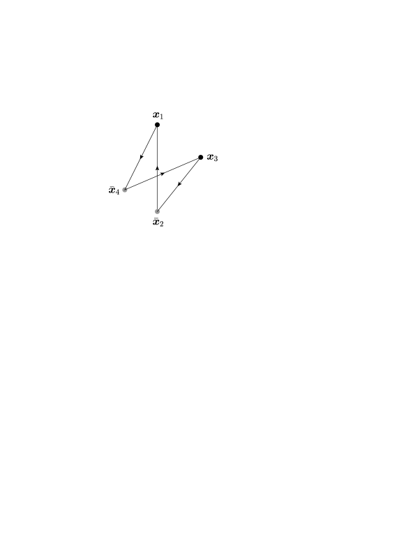
Figure 1: A pictorial representation of the color flow with the operator $\hat{Q}_{\bm{x}_{1}\bm{x}_{2}\bm{x}_{3}\bm{x}_{4}}$ (left) and respectively $\hat{Q}_{\bm{x}_{1}\bm{x}_{4}\bm{x}_{3}\bm{x}_{2}}$ (right).

By inspection of the higher equations in the Balitsky–JIMWLK equations, one can check that a similar symmetry holds for all the $n$–point functions of the Wilson lines. For instance, the equation obeyed by the sextupole $S$–matrix $\langle\hat{S}^{(6)}\rangle_{Y}$ is explicitly shown in Appendix B of Ref. Iancu:2011ns . From this equation, one can read the following symmetry property:

$$\langle\hat{S}_{\bm{x}_{1}\bm{x}_{2}\bm{x}_{3}\bm{x}_{4}\bm{x}_{5}\bm{x}_{6}}^{(6)}\rangle_{Y}\,=\,\langle\hat{S}_{\bm{x}_{1}\bm{x}_{6}\bm{x}_{5}\bm{x}_{4}\bm{x}_{3}\bm{x}_{2}}^{(6)}\rangle_{Y}\,.$$ (2.22)

The generalization of this property to the $2n$–point function shown in Eq. (2.9) reads

$$\langle\hat{S}_{\bm{x}_{1}\bm{x}_{2}...\bm{x}_{2n\!-\!2}\bm{x}_{2n\!-\!1}\bm{x}_{2n}}^{(2n)}\rangle_{Y}\,=\,\langle\hat{S}_{\bm{x}_{1}\bm{x}_{2n}\bm{x}_{2n\!-\!1}\bm{x}_{2n\!-\!2}...\bm{x}_{2}}^{(2n)}\rangle_{Y}\,.$$ (2.23)

To better understand the content of this symmetry, it is useful to give a pictorial representation for it. To that aim, consider a generic configuration of the quadrupole operator $\hat{Q}_{\bm{x}_{1}\bm{x}_{2}\bm{x}_{3}\bm{x}_{4}}$ in the transverse plane, as illustrated in Fig. 1, and join the four points by oriented lines, which follow the direction of color multiplication. In this way, one constructs a closed, oriented, contour, whose orientation indicates the flow of color within the operator. By repeating this procedure for the ‘permuted’ operator $\hat{Q}_{\bm{x}_{1}\bm{x}_{4}\bm{x}_{3}\bm{x}_{2}}$, one obtains a similar contour, where however the orientation of the color flow is reversed. One can similarly check that, for a general $n$–point function, the symmetry property (2.23) refers to changing the contour orientation, say from clockwise to counterclockwise. Such a change would also result from the reflection in a mirror, so we shall refer to the symmetry property (2.23) as the ‘mirror symmetry’. Additional arguments in the favor of this name will be given below.

There are several reasons why this this symmetry is so important for us here. First, as we shall shortly argue, this corresponds to an important symmetry property of the scattering amplitudes: their invariance under time–reversal. Second, the way how this symmetry is actually preserved by the JIMWLK evolution is very interesting as it sheds light on the physical picture of the target field distribution: with increasing $Y$, the color glass condensate expands symmetrically around $x^{-}=0$. Third, this symmetry will later guide us in the construction of a mean field approximation to the Balitsky–JIMWLK hierarchy.

                 

Figure 2: A different pictorial representation of the operators $\hat{Q}_{\bm{x}_{1}\bm{x}_{2}\bm{x}_{3}\bm{x}_{4}}$ (left) and $\hat{Q}_{\bm{x}_{1}\bm{x}_{4}\bm{x}_{3}\bm{x}_{2}}$ (right), which emphasizes the fact that they get exchanged with each other via time reversal, with ‘time’ $=x^{-}$.

To understand the relation to time–reversal, let us present another pictorial representation for the two quadrupole operators which enter Eq. (2.19): this is shown in Fig. 2, where the transverse space is schematically represented by the vertical axis, whereas the horizontal axis refers to $x^{-}$ — the light–cone time for the projectile. The Wilson lines are now explicitly shown, as the oriented horizontal lines extending along the $x^{-}$ axis and connected with each other, via matrix multiplication, at $x^{-}\to\pm\infty$. Once again, the orientation of these lines corresponds to the direction of the color flow. Clearly, these two figures get exchanged with each other when inverting the arrow of time. In the left figure, corresponding to $\hat{Q}_{\bm{x}_{1}\bm{x}_{2}\bm{x}_{3}\bm{x}_{4}}$, the 4–body system starts at $x^{-}\to-\infty$ as a set of 2 dipoles, $(\bm{x}_{1},\bm{x}_{2})$ and $(\bm{x}_{3},\bm{x}_{4})$, which then exchange color with each other at $x^{-}\to\infty$ and thus reconnect into the new dipoles $(\bm{x}_{1},\bm{x}_{4})$ and $(\bm{x}_{3},\bm{x}_{2})$. In the right figure, the opposite process happens: the system starts with the dipoles $(\bm{x}_{1},\bm{x}_{4})$ and $(\bm{x}_{3},\bm{x}_{2})$, which then reconnect at $x^{-}\to\infty$ into the dipoles $(\bm{x}_{1},\bm{x}_{2})$ and $(\bm{x}_{3},\bm{x}_{4})$, thus yielding the quadrupole $\hat{Q}_{\bm{x}_{1}\bm{x}_{4}\bm{x}_{3}\bm{x}_{2}}$. Hence, the symmetry property (2.19) corresponds indeed to invariance under time–reversal, as anticipated.

We now turn to the physical interpretation of the mirror symmetry in the context of the JIMWLK evolution. One can check that the symmetric structure of the virtual terms in Eq. (2.2) stems from the combined action of the first two terms in Eq. (2.2). Half of the ‘virtual’ terms are generated by the first term, proportional to the color unity matrix, but by themselves these terms do not show the mirror symmetry; this symmetry is recovered only after adding the other half of the ‘virtual’ terms, as generated by the second term in Eq. (2.2), proportional to $\widetilde{V}^{\dagger}_{\bm{u}}\widetilde{V}_{\bm{v}}$. As an example, consider two of the ‘virtual’ terms in the r.h.s. of Eq. (2.2) whose coefficients get exchanged with each other under the exchange $\bm{x}_{2}\leftrightarrow\bm{x}_{4}$ : $\mathcal{M}_{\bm{x}_{1}\bm{x}_{4}\bm{z}}\langle\hat{Q}_{\bm{x}_{1}\bm{x}_{2}\bm{x}_{3}\bm{x}_{4}}\rangle$ and $\mathcal{M}_{\bm{x}_{1}\bm{x}_{2}\bm{z}}\langle\hat{Q}_{\bm{x}_{1}\bm{x}_{2}\bm{x}_{3}\bm{x}_{4}}\rangle$. The first of them is generated when acting with the first term in the Hamiltonian on the pair ($\bm{x}_{1},\bm{x}_{4}$) of the quadrupole, whereas the second one emerges from the action of the second term in $H$ on the pair ($\bm{x}_{1},\bm{x}_{2}$).

Hence, to elucidate this symmetry, one needs to better understand the action of the JIMWLK Hamiltonian. As manifest from Eq. (2.11), the functional derivatives within the Hamiltonian act as generators of infinitesimal color rotations of the Wilson lines at their upper end point in $x^{-}$; that is, they act as Lie derivatives for the color group SU$(N_{c})$. These color rotations express the evolution of the target color field $\alpha_{a}(x^{-},\bm{x})$ with increasing rapidity: performing one infinitesimal step in the evolution, from $Y$ to $Y+{\rm d}Y$, amounts to ‘integrating out’ one layer of quantum fluctuations within the target wavefunction — the gluons with longitudinal momentum fractions between $x={\rm e}^{-Y}$ and $x^{\prime}={\rm e}^{-(Y+{\rm d}Y)}$ — and results in adding one additional layer to the classical color field $\alpha_{a}(x^{-},\bm{x})$. The fact that the JIMWLK Hamiltonian acts on the Wilson lines via color rotations at the largest value in $x^{-}$ means that the new layer of color field is located at larger $x^{-}$ as compared to the previous layers.

This argument makes it tempting to conclude that, with increasing $Y$, the support of the target field $\alpha_{a}(x^{-},\bm{x})$ extends only towards increasing $x^{-}$, thus yielding a field distribution which is asymmetric in $x^{-}$. This was indeed the prevailing viewpoint in the original literature on the JIMWLK evolution (see e.g. Iancu:2002xk ; Iancu:2003xm ), but now we shall argue that this is actually not quite right: although the functional derivatives in Eq. (2.2) have a one–sided action which amounts to color rotations at the largest value of $x^{-}$ alone, the overall structure of the Hamiltonian is such that the target field is nevertheless built symmetrically in $x^{-}$. In fact, it is precisely this symmetry of the target field distribution under reflection in $x^{-}$ which is responsible for the mirror symmetry in the evolution equations.

To see that, it is useful to notice that Eq. (2.2) can be alternatively rewritten as Kovner:2005jc ; Kovner:2005en

$$H=\frac{g^{2}}{16\pi^{3}}\int_{\bm{u}\bm{v}\bm{z}}\mathcal{M}_{\bm{u}\bm{v}\bm{z}}\Big{(}J_{L\bm{u}}^{a}J_{L\bm{v}}^{a}+J_{R\bm{u}}^{a}J_{R\bm{v}}^{a}+2\widetilde{V}_{\bm{z}}^{ab}J_{R\bm{u}}^{a}J_{L\bm{v}}^{b}\Big{)},$$ (2.24)

where $J_{L\bm{u}}^{a}$ and $J_{R\bm{v}}^{a}$ are functional differential operators acting as ‘left’ and ‘right’ Lie derivatives — that is, the generators of infinitesimal color rotations at the largest and, respectively, smallest value of $x^{-}$. They are defined as

$$J_{L\bm{u}}^{a}\,\equiv\,-\frac{1}{{\rm i}g}\,\frac{\delta}{\delta\alpha^{a}_{\bm{u}}}\,,\qquad J_{R\bm{u}}^{a}\,\equiv\,\frac{1}{{\rm i}g}\,\widetilde{V}_{\bm{u}}^{ab}\frac{\delta}{\delta\alpha^{b}_{\bm{u}}}\,,$$ (2.25)

and satisfy

$$J_{L\bm{u}}^{a}\,V_{\bm{x}}^{\dagger}\,=\,-\delta_{\bm{x}\bm{u}}\,t^{a}V_{\bm{x}}^{\dagger},\qquad J_{R\bm{u}}^{a}\,V_{\bm{x}}^{\dagger}\,=\,\delta_{\bm{x}\bm{u}}\,V_{\bm{x}}^{\dagger}t^{a},\,$$ (2.26)

where the second equation follows from the first one after using Eq. (2.14). These equations imply the following commutation relations

$$[J_{L\bm{u}}^{a},\,J_{L\bm{v}}^{b}]={\rm i}f^{abc}J_{L\bm{u}}^{c}\delta_{\bm{u}\bm{v}},\quad[J_{R\bm{u}}^{a},\,J_{R\bm{v}}^{b}]={\rm i}f^{abc}J_{R\bm{u}}^{c}\delta_{\bm{u}\bm{v}},\quad[J_{L\bm{u}}^{a},\,J_{R\bm{v}}^{b}]=0\,,$$ (2.27)

showing that the two sets of generators satisfy two independent SU$(N_{c})$ Lie algebras.

The physical interpretation of the various terms in Eq. (2.24) is quite transparent: the action of $J_{L\bm{u}}^{a}$ on the quark Wilson line $V_{\bm{x}}^{\dagger}$ (the first equation in Eq. (2.26)) amounts to the addition of an infinitesimal layer of color field at the largest values of $x^{-}$, whereas the action of $J_{R\bm{u}}^{a}$ is tantamount to a corresponding addition at the smallest values of $x^{-}$. Hence, the manifest symmetry of Eq. (2.24) under the exchange $L\leftrightarrow R$ implies that, during the high–energy evolution, the distribution of the target color field $\alpha^{a}(x^{-},\bm{x})$ — by which we mean its support and correlations — is built symmetrically in $x^{-}$ around $x^{-}=0$. Moreover, this is also the origin of the mirror symmetry since, as previously noticed, the latter follows from the combined action of the first two terms in the Hamiltonian (2.2), or (2.24) — those which get interchanged with each other under the permutation $L\leftrightarrow R$ of the Lie derivatives.

To better appreciate the differences between an evolution which is symmetric in $x^{-}$ and one which is not, it is instructive to consider the evolution of a Wilson line, say for a quark projectile. When computing the target average (2.5) with the CGC weight function at rapidity $Y$, the support of the color field $\alpha_{a}(x^{-},\bm{x})$ is restricted to $-x^{-}_{M}\leq x^{-}\leq x^{-}_{M}$ with $x^{-}_{M}(Y)=x^{-}_{0}\exp(Y-Y_{0})$. (This follows from the uncertainty principle: the softest gluon modes that have been integrated over have longitudinal momentum $p^{+}=xP$ with $x={\rm e}^{-Y}$, with $P=$ the total hadron momentum; hence, they are delocalized in $x^{-}$ over a distance $\sim 1/p^{+}\propto{\rm e}^{Y}$.) Thus, the quark Wilson line can be equivalently rewritten as

$${V}^{\dagger}_{\bm{x}}\,\equiv\,{\mbox{P}}\exp\left[{\rm i}g\int_{-x^{-}_{M}}^{x^{-}_{M}}{\rm d}x^{-}\alpha_{a}(x^{-},\bm{x})t^{a}\right].$$ (2.28)

This makes it manifest that, with increasing $Y$, the Wilson line ‘grows’ simultaneously at its both endpoints. To visualize the effect of one step in the evolution ($Y\to Y+{\rm d}Y$), it is useful to discretize rapidity by writing $Y_{n}=n\epsilon$, with $\epsilon$ an infinitesimal rapidity interval. Then under one additional step $n\to n+1$, the upper bound of the support extends as $x_{n}^{-}\equiv x^{-}_{M}(Y_{n})\to x^{-}_{n+1}=x_{n}^{-}(1+\epsilon)$ and the Wilson lines evolves as ${V}^{\dagger}_{n}\to{V}^{\dagger}_{n+1}$, with

$${V}^{\dagger}_{n+1}(\bm{x})=\exp[{\rm i}g\epsilon\alpha_{n+1}(\bm{x})]\,V_{n}^{\dagger}(\bm{x})\,\exp[{\rm i}g\epsilon\alpha_{-(n+1)}(\bm{x})]$$ (2.29)

where

$$\alpha_{n+1}(\bm{x})\equiv x_{n}^{-}\alpha_{a}(x^{-}_{n+1},\bm{x})t^{a}\quad\mbox{and}\quad\alpha_{-(n+1)}(\bm{x})\equiv x_{n}^{-}\alpha_{a}(-x^{-}_{n+1},\bm{x})t^{a}$$ (2.30)

represent the additional fields generated in this evolution step per unit of space–time rapidity. The infinitesimal gauge rotations associated with these new fields can be expanded in powers of $\epsilon$. Strictly speaking, this expansion must be pushed to quadratic order in $\epsilon$, to match with the fact that the evolution Hamiltonian (2.24) involves second order functional derivatives. However, the quadratic terms arising from the expansion of a given Wilson line do not contribute to the evolution of gauge–invariant observables: they would yield ‘tadpole’ contributions $\propto\delta_{\bm{u}\bm{v}}$, but the dipole kernel in the Hamiltonian vanishes when $\bm{u}=\bm{v}$. In other terms, the two functional derivatives within $H$ must act on different Wilson lines within the observable to give a non–zero result. So, we can restrict the expansion of (2.29) to linear order in $\epsilon$, which yields

$${V}^{\dagger}_{n+1}(\bm{x})-V_{n}^{\dagger}(\bm{x})={\rm i}g\epsilon\big{[}\alpha_{n+1}(\bm{x})\,V_{n}^{\dagger}(\bm{x})\,+\,V_{n}^{\dagger}(\bm{x})\alpha_{-(n+1)}(\bm{x})\big{]}+\mathcal{O}(\epsilon^{2})\,.$$ (2.31)

Clearly, the two terms in the r.h.s. correspond to the infinitesimal, ‘left’ and ‘right’, color rotations in Eq. (2.26). If instead of the symmetric evolution above, one would have considered an asymmetric one, where the target fields expands towards positive values of $x^{-}$ alone, the analog of Eqs. (2.29)–(2.31) would have involved the ‘left’ infinitesimal color precession alone.

In Ref. Blaizot:2002xy , the JIMWLK evolution has been reformulated as a random walk in the space of Wilson lines, which is formally such that one additional step corresponds to an infinitesimal rotation of ${V}^{\dagger}(\bm{x})$ on the ‘left’ alone. However, by inspection of the manipulations there, one can check that the additional contribution $\alpha_{n+1}(\bm{x})$ to the target field in the $(n+1)$th step is such that, in reality, that step simultaneously generate a color precession on the ‘left’ and on the ‘right’. That is, the Langevin process introduced in Ref. Blaizot:2002xy does in fact describe a symmetric evolution for the Wilson lines (or for the target field distribution), although this has not been recognized there.

3 The Gaussian approximation

In this section we shall demonstrate that the JIMWLK equation for the CGC weight function admits an approximate Gaussian solution which properly captures both the BFKL dynamics in the dilute regime at $k_{\perp}\gg Q_{s}(Y)$ and the approach towards the black disk limit in the saturation regime at $k_{\perp}\ll Q_{s}(Y)$. Our analysis improves over previous, related, constructions in the literature Iancu:2002xk ; Iancu:2002aq ; Kovchegov:2008mk at two important levels: (i) we actually justify the Gaussian approximation — including for the description of the higher–point correlation functions and for finite $N_{c}$ —, on the basis of the Balitsky–JIMWLK equations; (ii) we implement the ‘mirror’ symmetry discussed in Sect. 2.3, that is, we construct a Gaussian distribution which is symmetric in $x^{-}$ at any $Y$. As we shall see, this last condition is in fact compulsory to achieve a faithful description of the JIMWLK dynamics deeply at saturation.

The material of this section is organized as follows: the Gaussian weight function is introduced in Sect. 3.1, compared to the MV model in Sect. 3.2, and justified in Sects. 3.3 and 3.4 by comparison with piecewise approximations to the JIMWLK equations in the limiting regimes alluded to above.

3.1 The Gaussian weight function

The most general Gaussian weight function which is consistent with gauge symmetry and describes a target field distribution which is symmetric in $x^{-}$ reads

$$W_{Y}[\alpha]=\mathcal{N}_{Y}\exp\left[-\frac{1}{2}\int_{-x^{-}_{M}}^{x^{-}_{M}}{\rm d}x^{-}\!\int_{\bm{x}_{1}\bm{x}_{2}}\,{\alpha_{a}(x^{-},\bm{x}_{1})\bar{\gamma}^{-1}(x^{-},\bm{x}_{1},\bm{x}_{2})\alpha_{a}(x^{-},\bm{x}_{2})}\right]\delta_{Y}[\alpha]\,,$$ (3.1)

where $x^{-}_{M}(Y)=x^{-}_{0}\exp(Y-Y_{0})$ and the kernel $\bar{\gamma}^{-1}(x^{-},\bm{x}_{1},\bm{x}_{2})$ is an even function of $x^{-}$, assumed to be invertible. The functional $\delta$–function $\delta_{Y}[\alpha]$ ensures that the target field vanishes at larger longitudinal coordinates $|x^{-}|>x^{-}_{M}(Y)$ :

$$\delta_{Y}[\alpha]\,\equiv\,\prod_{|x^{-}|>x^{-}_{M}}\,\prod_{\bm{x}}\,\prod_{a}\,\delta(\alpha_{a}(x^{-},\bm{x}))\,.$$ (3.2)

Here, $\delta(\alpha_{a}(x^{-},\bm{x}))$ is the usual $\delta$–function and a discretization of the space–time is understood. Finally, the overall normalization factor $\mathcal{N}_{Y}$ in Eq. (3.1) is such that $\int{\mathcal{D}}\alpha\,W_{Y}[\alpha]=1$.

Eq. (3.1) implies that the only non–trivial correlation of the target fields is their 2–point function, which is moreover local in $x^{-}$ :

$$\langle\alpha_{a}(x^{-}_{1},\bm{x}_{1})\alpha_{b}(x^{-}_{2},\bm{x}_{2})\rangle_{Y}\,=\,\delta^{ab}\,\Theta\big{(}x^{-}_{M}(Y)-|x^{-}_{1}|\big{)}\,\delta(x^{-}_{1}-x^{-}_{2})\,\bar{\gamma}(x^{-}_{1},\bm{x}_{1},\bm{x}_{2})\,.$$ (3.3)

Within this Gaussian approximation, the locality in $x^{-}$ is required by gauge symmetry: to preserve the latter, any non–locality in $x^{-}$ should be accompanied by gauge links (Wilson lines) built with the field $\alpha^{a}$, which would spoil Gaussianity.

The Gaussian distribution (3.1) is manifestly symmetric in $x^{-}$ around $x^{-}=0$ and this symmetry is preserved by the high energy evolution. In fact, Eq. (3.1) depends upon $Y$ only via the two endpoints, $x^{-}_{M}(Y)$ and $-x^{-}_{M}(Y)$, of the support in $x^{-}$, meaning that the high–energy evolution proceeds via the symmetric expansion of the color field distribution towards both larger and smaller values of $x^{-}$. Specifically, by using the methods in Refs. Iancu:2002xk ; Blaizot:2002xy , one can check that the Gaussian weight function (3.1) obeys the following evolution equation:

$${\partial W_{Y}[\alpha]\over{\partial Y}}\,=\,{1\over 2}\int_{\bm{u}\bm{v}}\!\bar{\gamma}_{Y}(\bm{u},\bm{v})\,\left({\delta\over\delta\alpha^{a}_{L\bm{u}}}{\delta\over\delta\alpha^{a}_{L\bm{v}}}+{\delta\over\delta\alpha^{a}_{R\bm{u}}}{\delta\over\delta\alpha^{a}_{R\bm{v}}}\right)W_{Y}[\alpha]\,,$$ (3.4)

where the ‘left’ (‘right’) functional derivatives act on the target field at the largest (smallest) value of $x^{-}$, that is, at $x^{-}=x^{-}_{M}(Y)$ and respectively $x^{-}=-x^{-}_{M}(Y)$. Also $\bar{\gamma}_{Y}(\bm{x}_{1},\bm{x}_{2})$ denotes the field correlator per unit space–time rapidity as produced in the last step of the evolution,

$$\bar{\gamma}_{Y}(\bm{x}_{1},\bm{x}_{2})\equiv x^{-}_{M}\ \bar{\gamma}(\pm x^{-}_{M},\bm{x}_{1},\bm{x}_{2})\,.$$ (3.5)

Eq. (3.4) makes it manifest that the momentum rapidity and the space–time rapidity are identified with each other by the high–energy evolution. In order to solve Eq. (3.4), one also needs the generalization of Eq. (3.5) to intermediate values ${y}<Y$ for the space–time rapidity, that is

$$\bar{\gamma}_{y}(\bm{x}_{1},\bm{x}_{2})\equiv|x^{-}|\ \bar{\gamma}(x^{-},\bm{x}_{1},\bm{x}_{2})\,,\qquad\mbox{with}\qquad{y}\equiv Y_{0}+\,\ln\frac{|x^{-}|}{x^{-}_{0}}\,.$$ (3.6)

Eq. (3.4) should be viewed as a mean field approximation to the JIMWLK equation (2.1). It shows the same ‘left–right’ symmetry as the original equation, cf. Eq. (2.24), and hence it is consistent with the mirror symmetry discussed in Sect. 2.3. Clearly, this would not be the case if, instead of the symmetric Gaussian (3.1), one would consider an asymmetric one, say with support at $0\leq x^{-}\leq x^{-}_{M}(Y)$, as in the previous literature Iancu:2002xk ; Iancu:2002aq ; Kovchegov:2008mk : the corresponding evolution equation would contain only the ‘left’ functional derivatives — i.e., only the first term inside the brackets in Eq. (3.4).

To justify the Gaussian Ansatz (3.1) for the CGC weight function, we shall shortly compare the associated evolution equation (3.4) to the actual JIMWLK equation, in different kinematical regimes. In this process, we shall deduce piecewise approximations for the kernel $\bar{\gamma}_{Y}(\bm{x}_{1},\bm{x}_{2})$, valid at high ($k_{\perp}\gg Q_{s}(Y)$) and low ($k_{\perp}\ll Q_{s}(Y)$) momenta, respectively.

3.2 The McLerran–Venugopalan model

Before we turn to the JIMWLK evolution, let us briefly discuss the McLerran–Venugopalan (MV) model McLerran:1993ni ; McLerran:1993ka that we shall take as our initial condition at rapidity $Y_{0}$. Besides providing the initial conditions, this model (and its ad–hoc extrapolation towards high–energy) will serve as a baseline of comparison for the mean–field results that we shall later obtain. Its discussion will also give us an opportunity to clarify some subtle aspects of the Gaussian approximation, like the gauge artifacts in the ‘$\alpha$–representation’, cf. Eq. (3.1).

In the MV model one assumes that the color charges in the nucleus are uncorrelated valence quarks. Accordingly the distribution of the color charge density $\rho^{a}(x^{-},\bm{x})$ is a Gaussian with a kernel which is local in the transverse plane:

$$W_{Y_{0}}[\rho]\,=\,\mathcal{N}_{Y_{0}}\,\exp\left[-\frac{1}{2}\int_{-x^{-}_{0}}^{x^{-}_{0}}{\rm d}x^{-}\!\int_{\bm{x}}\,\frac{\rho^{a}(x^{-},\bm{x})\rho^{a}(x^{-},\bm{x})}{\lambda(x^{-},\bm{x})}\right]\,\delta_{Y_{0}}[\rho]\,,$$ (3.7)

where of course $\lambda(-x^{-},\bm{x})=\lambda(x^{-},\bm{x})$. Eq. (3.7) implies:

$$\langle\rho_{a}(x^{-}_{1},\bm{x}_{1})\rho_{b}(x^{-}_{2},\bm{x}_{2})\rangle_{Y}\,=\,\delta_{ab}\,\Theta\big{(}x^{-}_{0}-|x^{-}_{1}|\big{)}\,\delta(x^{-}_{1}-x^{-}_{2})\,\delta_{\bm{x}_{1}\bm{x}_{2}}\,\lambda(x^{-}_{1},\bm{x}_{1})\,.$$ (3.8)

The quantity $\lambda(x^{-},\bm{x})$ has the meaning of color charge squared per unit transverse area per unit longitudinal distance. In general the nucleus is assumed to be homogeneous in the transverse plane, i.e. the kernel in Eq. (3.7) is taken to be independent of $\bm{x}$. Under that assumption, the calculation of expectation values in the MV model is not sensitive to the detailed dependence of the kernel upon $x^{-}$, but only to its integral

$$\mu^{2}\equiv\int_{-x^{-}_{0}}^{x^{-}_{0}}{\rm d}x^{-}\lambda(x^{-})\,=\,2\int_{-\infty}^{Y_{0}}{\rm d}{y}\,\lambda_{y}=\,\frac{g^{2}A}{2\pi R_{A}^{2}}\,,$$ (3.9)

which physically represents the color charge squared per unit area. In the above equation, the quantity $\lambda_{y}\equiv|x^{-}|\lambda(x^{-})$ (the strength of the charge correlator per unit space–time rapidity) has been defined by analogy with Eq. (3.6). The last equality follows after counting the color charges of the valence quarks within a nucleus with atomic number $A$ and transverse area $\pi R_{A}^{2}$ (see e.g. Iancu:2003xm ). The fact that it is only the integrated quantity (3.9) which matters arises from the fact that, under the present assumptions, the charge correlator (3.8) is separable as a function of $x^{-}$ and the transverse coordinates. We shall return to this issue in Sects. 4.2 and 4.3.

Eq. (3.7) is gauge invariant, but in order to make contact with the $\alpha$–representation that we use throughout this paper, we shall henceforward consider it within the class of gauges where the target field is of the form $A^{\mu}_{a}=\delta^{\mu+}\alpha_{a}$. Then $\alpha_{a}(x^{-},\bm{x})$ is related to the color charge density $\rho_{a}(x^{-},\bm{x})$ via the 2–dimensional Coulomb equation: $-\nabla^{2}_{\perp}\alpha_{a}=\rho_{a}$. So, for a homogeneous target, Eq. (3.8) implies the following expression for the 2–point function for the color field, in transverse momentum space (we denote ${\bm{r}}=\bm{x}_{1}-\bm{x}_{2}$ and $k_{\perp}=|\bm{k}|$):

$$\bar{\gamma}_{y}(\bm{k})\,\equiv\int{{\rm d}^{2}{\bm{r}}}\,{\rm e}^{{\rm i}\bm{k}\,\mspace{-2.0mu}\cdot\mspace{-2.0mu}\,{\bm{r}}}\,\bar{\gamma}_{y}({\bm{r}})\,=\,\frac{\lambda_{y}}{k_{\perp}^{4}}\quad\mbox{for}\quad{y}\,\leq\,Y_{0}\,.$$ (3.10)

Here and from now on, we prefer to work with the expressions of the various correlators per unit space–time rapidity, cf. Eq. (3.6), since these are the expressions which most directly enter the mean–field evolution equations like (3.4).

Eq. (3.10) raises a potential problem: the Fourier transform of this expression back to the transverse coordinate space is not well defined, as it involves a (quadratic) infrared divergence. This problem reflects the fact that, by itself, the field $\alpha_{a}(x^{-},\bm{x})$ is not invariant under the residual gauge transformations which preserve the structure $A^{\mu}_{a}=\delta^{\mu+}\alpha_{a}$ for the target field. The infinitesimal version of such a transformation reads $\alpha_{a}(x^{-},\bm{x})\to\alpha_{a}(x^{-},\bm{x})+\partial^{+}\omega_{a}(x^{-})$, with $\omega_{a}(x^{-})$ an arbitrary function Hatta:2005as ; so, clearly, the color charge density $\rho_{a}(x^{-},\bm{x})$ is invariant under this transformation. Strictly speaking, the general weight function $W_{Y}$ (and, in particular, its Gaussian approximation, Eq. (3.1)) should be written as a functional of $\rho$, to make gauge symmetry manifest. On the other hand, observables like scattering amplitudes are built with Wilson lines, which are path–ordered exponentials of $\alpha$. Taken separately, one Wilson line is not gauge invariant (rather, it transforms via color rotations Hatta:2005as ), but the physically relevant operators, which involve a product of such lines, cf. Eq. (2.9), are invariant. Whenever computing the expectation value of such a gauge–invariant operator, there is no problem with using the weight function in the $\alpha$–representation, as given in Eq. (3.1): all the gauge artifacts cancel out in the final result.

As an example, consider the calculation of the dipole $S$–matrix within the MV model. The corresponding result is well known and reads (see also Sect. 4.2)

$$\langle\hat{S}_{\bm{x}_{1}\bm{x}_{2}}\rangle_{Y_{0}}={\rm e}^{-\Gamma_{Y_{0}}(\bm{x}_{1},\bm{x}_{2})}$$ (3.11)

where we have assumed the MV model to apply at all the rapidities $Y\leq Y_{0}$ and we defined

$$\Gamma_{Y_{0}}(\bm{x}_{1},\bm{x}_{2})={g^{2}C_{F}}\int^{Y_{0}}_{-\infty}{\rm d}{y}\,\left[\bar{\gamma}_{y}(\bm{x}_{1},\bm{x}_{1})+\bar{\gamma}_{y}(\bm{x}_{2},\bm{x}_{2})-2\bar{\gamma}_{y}(\bm{x}_{1},\bm{x}_{2})\right],$$ (3.12)

with $C_{F}={(N_{c}^{2}-1)}/{2N_{c}}$. Eq. (3.12) involves only the following linear combination of the target field correlators

$$\gamma_{y}(\bm{x}_{1},\bm{x}_{2})\equiv-\bar{\gamma}_{y}(\bm{x}_{1},\bm{x}_{2})+\frac{1}{2}\big{[}\bar{\gamma}_{y}(\bm{x}_{1},\bm{x}_{1})+\bar{\gamma}_{y}(\bm{x}_{2},\bm{x}_{2})\big{]}=\int\frac{{\rm d}^{2}\bm{k}}{(2\pi)^{2}}\frac{\lambda_{y}}{k_{\perp}^{4}}\Big{[}1-{\rm e}^{{\rm i}\bm{k}\,\mspace{-2.0mu}\cdot\mspace{-2.0mu}\,(\bm{x}_{1}-\bm{x}_{2})}\Big{]}.$$ (3.13)

which is gauge–invariant, since under a residual gauge transformation the target field $\alpha^{a}(x^{-},\bm{x})$ changes by a $\bm{x}$–independent quantity. The sign in the r.h.s. of Eq. (3.13) is such that $\gamma_{y}(\bm{x}_{1},\bm{x}_{2})$ be positive–semidefinite. The last equality in Eq. (3.13), which involves the color charge correlator $\lambda_{y}$, illustrates the fact that the infrared divergences due to gauge artifacts cancel out in the linear combination (3.13). Strictly speaking, the above integral over $\bm{k}$ still has a logarithmic infrared divergence, but this is milder than the quadratic divergence appearing in the Fourier transform of $\bar{\gamma}_{y}(\bm{k})$ in Eq. (3.10). The remaining divergence is not a gauge artifact anymore, but a ‘physical’ singularity of this model: it reflects the lack of correlations among the color sources. After taking into account the high–energy evolution, transverse correlations get built which screen out this divergence, as we shall shortly see. For completeness, let us estimate the final integral in Eq. (3.12): introducing an infrared cutoff $\Lambda$ to regularize the remaining infrared divergence and writing $r=|\bm{x}_{1}-\bm{x}_{2}|$, one finds

$$\Gamma_{Y_{0}}(r)={g^{2}C_{F}}\,\frac{g^{2}A}{2\pi R_{A}^{2}}\,\int\frac{{\rm d}^{2}\bm{k}}{(2\pi)^{2}}\frac{1-{\rm e}^{{\rm i}\bm{k}\,\mspace{-2.0mu}\cdot\mspace{-2.0mu}\,{\bm{r}}}}{k_{\perp}^{4}}\,\simeq\,\frac{r^{2}Q_{0}^{2}}{4}\,\ln\frac{1}{r^{2}\Lambda^{2}}\,,$$ (3.14)

where $Q_{0}^{2}\equiv 2\alpha_{s}^{2}C_{F}A/R_{A}^{2}$ is essentially the nuclear saturation scale (as probed by a quark–antiquark dipole) at the initial rapidity $Y_{0}$. Although obtained within the MV model, the above results are generic in the following sense: all the gauge–invariant observables computed in the Gaussian approximation involve the kernel $\bar{\gamma}_{y}(\bm{x}_{1},\bm{x}_{1})$ of the Gaussian (the correlator of the target color field) only via the linear combination shown in Eq. (3.13). So, in practice, there is no problem with using the $\alpha$–representation, as shown in Eq. (3.1).

Let us conclude this subsection with a remark on the calculation of expectation values within the MV model. The similarity between the respective weight function, Eq. (3.7), and the Gaussian approximation to the JIMWLK evolution, Eq. (3.1), makes it clear that one can consider the MV model as the result of a fictitious ‘evolution’ in which the target charge distribution is built in layers of $x^{-}$, from $x^{-}=0$ up to $|x^{-}|=x^{-}_{0}$. Specifically, let $W_{X^{-}}[\rho]$ denote the generalization of Eq. (3.7) in which $x^{-}_{0}$ is replaced by $X^{-}$ and assume the nucleus to be homogeneous in the transverse plane. Then Eq. (3.7) is the solution to the following, functional, evolution equation (compare to Eq. (3.4))

$${\partial W_{X^{-}}[\rho]\over{\partial{X^{-}}}}\,=\,{1\over 2}\,\lambda_{X^{-}}\int_{\bm{u}\bm{v}}\!\left({\delta\over\delta\rho^{a}_{L\bm{u}}}{\delta\over\delta\rho^{a}_{L\bm{v}}}+{\delta\over\delta\rho^{a}_{R\bm{u}}}{\delta\over\delta\rho^{a}_{R\bm{v}}}\right)W_{X^{-}}[\rho]\,,$$ (3.15)

integrated from $X^{-}=0$ up to $X^{-}=x^{-}_{0}$. In this equation, $\rho^{a}_{L}$ and $\rho^{a}_{R}$ refer to the color charge densities at $x^{-}=X^{-}$ and $x^{-}=-X^{-}$, respectively. When applied to the evolution of the Wilson–line correlations, Eq. (3.15) amounts to constructing the Wilson lines via symmetric iterations, i.e. via infinitesimal color precessions which proceed simultaneously ‘on the left’ and ‘on the right’, as shown in Eq. (2.29). However, within the context of the MV model, this symmetric iteration is merely a choice of a discretization prescription and any other choice is equally good. As a matter of fact, the common choice in the literature in this context (see e.g. Kovner:2001vi ; Blaizot:2004wv ; JalilianMarian:2004da ; Dominguez:2011wm ) is to perform asymmetric iterations ‘on the left’ :

$${V}^{\dagger}_{n}(\bm{x})\,\to\,{V}^{\dagger}_{n+1}(\bm{x})=\exp[{\rm i}g\epsilon\alpha_{n+1}(\bm{x})]\,V_{n}^{\dagger}(\bm{x}),$$ (3.16)

where this time $n$ refers to a discretization of the $x^{-}$ axis. This procedure is tantamount to solving the following evolution equation

$${\partial W_{X^{-}}[\rho]\over{\partial{X^{-}}}}\,=\,{1\over 2}\,\lambda_{X^{-}}\int_{\bm{u}\bm{v}}{\delta\over\delta\rho^{a}_{L\bm{u}}}{\delta\over\delta\rho^{a}_{L\bm{v}}}W_{X^{-}}[\rho]\,,$$ (3.17)

from $X^{-}=-x_{0}^{-}$ up to $X^{-}=x^{-}_{0}$. In practice, one often takes $x^{-}_{0}\to\infty$, since the results are anyway insensitive to the actual value of $x^{-}_{0}$, but only depend upon the integral $\int{\rm d}X^{-}\lambda(X^{-})$.

The above discussion sheds more light on the role of the ‘left–right’ symmetry in the evolution equations. So long as the CGC weight function is given (like in the MV model) and the associated evolution equations are merely used as a convenient device to compute expectation values, the symmetric discretization in Eq. (2.29) is not compulsory and it might not even be the most convenient one in practice. However, for the JIMWLK equation and any (mean field) approximation to it, the symmetric iteration is the only one to be correct, since this is how the target field distribution gets actually built via quantum evolution: the ‘outer’ layers (those located at larger values of $|x^{-}|$) are constructed after the ‘inner’ ones (those at smaller $|x^{-}|$), and the new correlations built in one step depend upon the color field produced in all the previous steps. Hence, it would make no sense to consider an asymmetric evolution, like Eq. (3.17), since this would violate causality in the domain of negative $x^{-}$.

3.3 Weak–scattering regime: the BFKL dynamics

In what follows, we shall study the JIMWLK evolution in two limiting regimes — large transverse momenta $k_{\perp}\gg Q_{s}(Y)$ in this section and relatively small momenta $k_{\perp}\ll Q_{s}(Y)$ in the next subsection — with the purpose of showing that, in both regimes, the evolution is consistent with a mean field approximation of the type shown in Eq. (3.4). We recall that $Q_{s}(Y)$ is the saturation momentum in the target (in a frame in which the target carries most of the total rapidity separation $Y$) and it increases with $Y$ very fast. For a multi–point correlation function like the quadrupole (2.8), the statement that the ‘transverse momenta are much larger than $Q_{s}$’ means that all the transverse separations $r_{ij}\equiv|\bm{x}_{i}-\bm{x}_{j}|$ between the external points are much smaller than $1/Q_{s}(Y)$. Similarly, by ‘momenta much smaller than $Q_{s}$’, we mean that $r_{ij}\gg 1/Q_{s}(Y)$ for any pair $(\bm{x}_{i},\bm{x}_{j})$ of external points. Very asymmetric configurations, where some of the distances $r_{ij}$ are much larger than $1/Q_{s}(Y)$ while the others are much smaller, are strictly speaking not covered by the present analysis and must be separately studied. We shall discuss some examples of that kind in Sect. 4.4 below.

For high transverse momenta $k_{\perp}\gg Q_{s}(Y)$, the gluon density in the target is low, meaning that the corresponding color field is weak: $g\int{\rm d}x^{-}\alpha\ll 1$. It is then possible to expand the Wilson lines to lowest non–trivial order in the field in their exponent, within both the JIMWLK Hamiltonian and the operators defining the observables. For an operator like the dipole $S$–matrix Eq. (2.7), we need to push the expansion in $g\alpha$ up to the second order, since the linear terms vanish after averaging. Introducing the dipole $T$–matrix operator $\hat{T}_{\bm{x}_{1}\bm{x}_{2}}\equiv 1-\hat{S}_{\bm{x}_{1}\bm{x}_{2}}$, whose expectation value represents the corresponding scattering amplitude, this expansion yields

$$\langle\hat{T}_{\bm{x}_{1}\bm{x}_{2}}\rangle_{Y}\,\simeq\,\frac{g^{2}}{4N_{c}}\langle(\alpha_{\bm{x}_{1}}^{a}-\alpha_{\bm{x}_{2}}^{a})^{2}\rangle_{Y}\qquad\mbox{with}\qquad\alpha^{a}_{\bm{x}}\,\equiv\,\int{\rm d}x^{-}\alpha_{a}(x^{-},\bm{x})\,.$$ (3.18)

The weak scattering regime corresponds to $\langle\hat{T}\rangle_{Y}\ll 1$. Note that Eq. (3.18) involves only the linear combination (3.13) of the target field correlators, in agreement with the discussion in Sect. 3.2. The similar expansion for the quadrupole $S$–matrix, Eq. (2.8), yields

$$1-\langle\hat{Q}_{\bm{x}_{1}\bm{x}_{2}\bm{x}_{3}\bm{x}_{4}}\rangle_{Y}\simeq\langle\hat{T}_{\bm{x}_{1}\bm{x}_{2}}-\hat{T}_{\bm{x}_{1}\bm{x}_{3}}+\hat{T}_{\bm{x}_{1}\bm{x}_{4}}+\hat{T}_{\bm{x}_{2}\bm{x}_{3}}-\hat{T}_{\bm{x}_{2}\bm{x}_{4}}+\hat{T}_{\bm{x}_{3}\bm{x}_{4}}\rangle_{Y},$$ (3.19)

where it is understood that $\langle\hat{T}\rangle_{Y}$ is evaluated according to Eq. (3.18). More generally, in this dilute regime, all the $n$–point functions of the type shown in Eqs. (2.9) or (2.10) reduce to linear combinations of dipole amplitudes. This already shows that a Gaussian approximation for the CGC weight function should be indeed possible, to the accuracy of interest. To identify this approximation, let us also consider the weak–field limit of the JIMWLK Hamiltonian. Its obtention is facilitated by observing that Eq. (2.2) can be rewritten as

$$1+\widetilde{V}^{\dagger}_{\bm{u}}\widetilde{V}_{\bm{v}}-\widetilde{V}^{\dagger}_{\bm{u}}\widetilde{V}_{\bm{z}}-\widetilde{V}^{\dagger}_{\bm{z}}\widetilde{V}_{\bm{v}}\,=\,\left(1-\widetilde{V}^{\dagger}_{\bm{u}}\widetilde{V}_{\bm{z}}\right)\,\left(1-\widetilde{V}^{\dagger}_{\bm{z}}\widetilde{V}_{\bm{v}}\right)\,.$$ (3.20)

The leading order terms in the dilute regime are then obtained by expanding the Wilson lines within each of the two parentheses above to linear order in $g\alpha$. (This amounts to an expansion of the original structure in the l.h.s. of Eq. (3.20) up to quadratic order.) For instance,

$$1-\widetilde{V}^{\dagger}_{\bm{u}}\widetilde{V}_{\bm{z}}\,\simeq\,-{\rm i}g\big{(}\alpha^{a}_{\bm{u}}-\alpha^{a}_{\bm{z}}\big{)}T^{a}\,,$$ (3.21)

with $\alpha^{a}_{\bm{u}}$ as defined in Eq. (3.18). After also using $(T^{a})_{bc}={\rm i}f^{abc}$, one finds $H\simeq H_{\rm BFKL}$ with

$$H_{\rm BFKL}=-\,\frac{g^{2}}{16\pi^{3}}\int_{\bm{u}\bm{v}\bm{z}}{\mathcal{M}}_{\bm{u}\bm{v}\bm{z}}\big{(}\alpha^{a}_{\bm{u}}-\alpha^{a}_{\bm{z}}\big{)}\big{(}\alpha^{b}_{\bm{z}}-\alpha^{b}_{\bm{v}}\big{)}\,f^{acf}f^{bfd}\frac{\delta}{\delta\alpha^{c}_{\bm{u}}}\frac{\delta}{\delta\alpha^{d}_{\bm{v}}}\,.$$ (3.22)

This Hamiltonian is supposed to act on operators which are themselves evaluated in the weak–scattering regime and hence are quadratic functions of the field $\alpha_{\bm{x}}^{a}$, as illustrated in (3.18) and (3.19). Clearly, the only evolution equation of interest for us here is that obeyed by the dipole scattering amplitude (3.18). This is readily obtained as

$$\frac{\partial\langle\hat{T}_{\bm{x}_{1}\bm{x}_{2}}\rangle_{Y}}{\partial Y}=\frac{\bar{\alpha}}{2\pi}\,\int_{\bm{z}}\mathcal{M}_{\bm{x}_{1}\bm{x}_{2}\bm{z}}\,\big{\langle}\hat{T}_{\bm{x}_{1}\bm{z}}+\hat{T}_{\bm{z}\bm{x}_{2}}-\hat{T}_{\bm{x}_{1}\bm{x}_{2}}\big{\rangle}_{Y}\,,$$ (3.23)

and is recognized as the BFKL equation Lipatov:1976zz ; Kuraev:1977fs ; Balitsky:1978ic , that is, the equation obtained after linearizing Eq. (2.16) with respect to $\langle\hat{T}\rangle_{Y}$. By using its solution, one can compute any other $n$–point function of the Wilson lines, like Eq. (3.19), in this dilute regime.

We now construct the Gaussian approximation which reproduces the BFKL equation. To that aim, we shall compare the mean–field equation for $\langle\hat{T}_{\bm{x}_{1}\bm{x}_{2}}\rangle_{Y}$ generated by Eq. (3.4) with Eq. (3.23) and thus deduce an approximate expression for $\bar{\gamma}_{Y}(\bm{u},\bm{v})$ valid in this linear regime. Notice that the left and right functional derivatives yield identical results when acting on the field $\alpha_{\bm{x}}^{a}$ which is integrated over $x^{-}$. Hence, Eqs. (3.4) and (3.18) imply

$$\frac{\partial\langle\hat{T}_{\bm{x}_{1}\bm{x}_{2}}\rangle_{Y}}{\partial Y}\bigg{|}_{\rm MFA} =\frac{g^{2}}{4N_{c}}\int_{\bm{u}\bm{v}}\!\bar{\gamma}_{Y}(\bm{u},\bm{v})\,\Big{\langle}{\delta\over\delta\alpha^{b}_{\bm{u}}}{\delta\over\delta\alpha^{b}_{\bm{v}}}(\alpha_{\bm{x}_{1}}^{a}-\alpha_{\bm{x}_{2}}^{a})^{2}\Big{\rangle}_{Y}$$

$$=\frac{g^{2}}{4N_{c}}\,2\delta^{aa}\,\left[\bar{\gamma}_{Y}(\bm{x}_{1},\bm{x}_{1})+\bar{\gamma}_{Y}(\bm{x}_{2},\bm{x}_{2})-2\bar{\gamma}_{Y}(\bm{x}_{1},\bm{x}_{2})\right]$$

$$=g^{2}\frac{N_{c}^{2}-1}{N_{c}}\,\gamma_{Y}(\bm{x}_{1},\bm{x}_{2})\,,$$ (3.24)

with $\gamma_{Y}(\bm{x}_{1},\bm{x}_{2})$ defined as in Eq. (3.13). The last equation can be integrated to yield

$$\langle\hat{T}_{\bm{x}_{1}\bm{x}_{2}}\rangle_{Y}\Big{|}_{\rm MFA}=2g^{2}C_{F}\,f_{Y}(\bm{x}_{1},\bm{x}_{2})\quad\mbox{with}\quad f_{Y}(\bm{x}_{1},\bm{x}_{2})\equiv\int_{-\infty}^{Y}{\rm d}{y}\,\gamma_{y}(\bm{x}_{1},\bm{x}_{2})\,.$$ (3.25)

It is easy to check that the same expression for $\langle\hat{T}\rangle_{Y}$ would be obtained by directly evaluating the expectation value in Eq. (3.18) with the help of Eq. (3.3). But its above derivation via the mean–field equation of motion has the merit to emphasize that the evolution equations for gauge–invariant observables generated by the Gaussian approximation involve the well–behaved kernel $\gamma_{Y}(\bm{x}_{1},\bm{x}_{2})$ in spite of the fact that the corresponding functional equation (3.4) features the (generally ill defined) kernel $\bar{\gamma}_{Y}(\bm{x}_{1},\bm{x}_{2})$. This property is generic: it holds beyond the present, BFKL, approximation. Thus, for all practical purposes one can replace $\bar{\gamma}_{Y}(\bm{u},\bm{v})\to-\gamma_{Y}(\bm{u},\bm{v})$ within Eq. (3.4). This replacement works in the same way as that of the original kernel in the JIMWLK equation Weigert:2000gi ; Iancu:2001ad ; Ferreiro:2001qy by the dipole kernel in Eq. (2.2): the new kernel is to be used only when acting on gauge–invariant observables and it has the property to vanish at $\bm{u}=\bm{v}$.

Returning to the mean–field expression (3.25) for $\langle\hat{T}\rangle_{Y}$, this must be consistent with the BFKL equation (3.23). This is clearly the case provided the function $f_{Y}(\bm{x}_{1},\bm{x}_{2})$ itself satisfies the BFKL equation:

$$\frac{\partial f_{Y}(\bm{x}_{1},\bm{x}_{2})}{\partial Y}=\frac{\bar{\alpha}}{2\pi}\,\int_{\bm{z}}\mathcal{M}_{\bm{x}_{1}\bm{x}_{2}\bm{z}}\left[f_{Y}(\bm{x}_{1},\bm{z})+f_{Y}(\bm{z},\bm{x}_{2})-f_{Y}(\bm{x}_{1},\bm{x}_{2})\right]\,.$$ (3.26)

The initial conditions for the above equations can be taken from the MV model, which yields (for $r\ll 1/Q_{0}$) : $\langle\hat{T}(r)\rangle_{Y_{0}}=2g^{2}C_{F}\,f_{Y_{0}}(r)=\Gamma_{Y_{0}}(r)$, with $\Gamma_{Y_{0}}$ given in Eq. (3.14).

The solution to Eq. (3.26) is by now well understood. Here we will just remind that the BFKL evolution introduces transverse correlations between the ‘color sources’ (radiated gluons) which ensure that the solution $f_{Y}(\bm{x}_{1},\bm{x}_{2})$ becomes infrared finite after a rapidity evolution $Y-Y_{0}\sim 1/\bar{\alpha}$. In particular, in the window for ‘extended geometric scaling’ Iancu:2002tr ; Mueller:2002zm ; Munier:2003vc , which holds for transverse momenta relatively close to (but still larger than) the saturation momentum $Q_{s}(Y)$, one has $\lambda_{Y}(\bm{k})=k_{\perp}^{4}\gamma_{Y}(\bm{k})\propto k_{\perp}^{2(1-\gamma_{s})}$ with $\gamma_{s}\approx 0.63$ (the ‘BFKL anomalous dimension at saturation’). Then, clearly, the integral over $\bm{k}$ in Eq. (3.13) is well defined when computed within the BFKL approximation.

To summarize, the mean–field equation (3.4), where it is understood that the kernel can be replaced as $\bar{\gamma}_{Y}\to-\gamma_{Y}$ with the function $\gamma_{Y}(\bm{u},\bm{v})$ determined by Eq. (3.26), properly encodes the BFKL evolution of the dipole amplitude in the weak scattering regime. This conclusion holds for any value of the number of colors $N_{c}$ and it extends to all the $n$–point functions like (2.9) and (2.10) which, in this regime, reduce to linear combinations of dipole amplitudes.

Before concluding this section, let us recall that there are also other aspects of the BFKL dynamics, which cannot be encoded into a Gaussian weight function. They refer to operators more complicated than those in Eq. (2.9), which already at weak scattering involve more than two gluon exchanges; that is, to lowest order in the weak field expansion, they involve polynomials in $\alpha$ of a degree higher than two. (Such operators can be obtained e.g. by subtracting the dipolar contributions to the Wilson–line operators in Eqs. (2.9)–(2.10).) An example of that type is the ‘odderon’ operator, which describes $C$–odd exchanges and which in perturbation theory starts with three gluon exchanges. The corresponding evolution equation is correctly encoded (to leading logarithmic accuracy) in the JIMWLK equation Hatta:2005as — in particular, its low–density limit, known as the ‘BKP equation’ Bartels:1980pe ; Kwiecinski:1980wb ; Jaroszewicz:1980mq , is generated by the weak–field limit (3.22) of the JIMWLK Hamiltonian Hatta:2005as — but this description goes beyond the purpose of a Gaussian approximation, which by construction can encode only the 2–point function of the $\alpha$ field. For instance, to describe odderon effects in the initial conditions, one needs an extension of the MV model allowing for a non–trivial 3–point function Jeon:2005cf .

What is however remarkable about the Gaussian approximation that we pursue here is its capacity to encode non–trivial correlations among $n$ Wilson lines with arbitrary $n$ in the strong scattering regime, where the linear relation between the $n$–point functions and the 2–point function does not hold anymore. This will be discussed in the next subsection.

3.4 Strong–scattering regime: the dominance of the ‘virtual’ terms

For relatively low transverse momenta $k_{\perp}\lesssim Q_{s}(Y)$, the gluon occupation numbers in the target wavefunction saturate at a large value of order $1/\alpha_{s}$, meaning that $g\int{\rm d}x^{-}\alpha\sim\mathcal{O}{(1)}$. This in turn implies that the scattering is strong for projectiles with transverse sizes $r\gtrsim 1/Q_{s}$. For instance, the dipole scattering amplitude $\langle\hat{T}_{\bm{x}_{1}\bm{x}_{2}}\rangle_{Y}$ becomes of order one when $|\bm{x}_{1}-\bm{x}_{2}|\gtrsim 1/Q_{s}$. Then Eq. (3.19) implies that, for generic configurations at least, the quadrupole scattering becomes strong when at least one (which necessarily means at least three) of the six transverse distances $r_{ij}=|\bm{x}_{i}-\bm{x}_{j}|$ is of order $1/Q_{s}$, or larger. Similar considerations apply to the higher–point correlations. In this regime, the Wilson lines cannot be expanded out anymore. Rather, they resum multiple scattering to all orders in the eikonal approximation.

To correctly describe the high–energy evolution in the presence of gluon saturation and multiple scattering, it is of course essential to keep the non–linear terms in the Balitsky–JIMWLK equations, so like $\langle\hat{S}\hat{S}\rangle_{Y}$ in the equation (2.16) for the dipole $S$–matrix and $\langle\hat{S}\hat{Q}\rangle_{Y}$ in the r.h.s. of Eq. (2.2) for the quadrupole. In fact, these are precisely the terms responsible for the approach towards saturation in the gluon distribution and towards unitarity in the scattering of the projectile. Accordingly, in the transition regime towards saturation/unitarity (i.e. for $k_{\perp}\sim Q_{s}(Y)$), one has to deal with the whole, infinite, hierarchy of coupled evolution equations: no simple mean–field approximation (like a Gaussian) is possible in that regime. However, the situation drastically simplifies deeply at saturation ($k_{\perp}\ll Q_{s}(Y)$), where the only role of the non–linear terms in the equation is to forbid further evolution — or, more correctly, to limit the transverse phase–space for the high–energy evolution: gluons with soft momenta $k_{\perp}\ll Q_{s}(Y)$ can (almost) not be emitted anymore, meaning that domains separated by transverse distances $r\gg 1/Q_{s}(Y)$ evolve independently from each other. This leads to considerable simplifications in the Balitsky–JIMWLK equations, which can be most directly recognized by inspection of the projectile evolution.

For multi–partonic projectiles which are such that all the interparticle separations $r_{ij}$ are much larger than $1/Q_{s}(Y)$, the associated $S$–matrices are very small (close to zero) — the more so the larger the number of partons. Roughly speaking, and up to subtleties related to the $1/N_{c}^{2}$ corrections to which we shall later return, a 2–dipole projectile scatters more strongly than a single–dipole one, $\langle\hat{S}\hat{S}\rangle_{Y}\ll\langle\hat{S}\rangle_{Y}$, a projectile made with a dipole plus a quadrupole scatters more strongly than the quadrupole alone, $\langle\hat{S}\hat{Q}\rangle_{Y}\ll\langle\hat{Q}\rangle_{Y}$, etc. When this happens, the ‘virtual’ terms dominate the evolution, whereas the ‘real’ terms can be simply replaced with a lower cutoff $\sim 1/Q_{s}(Y)$ on the transverse separation $|\bm{z}-\bm{x}_{i}|$ between the newly emitted gluon at $\bm{z}$ and any of the preexisting partons at $\bm{x}_{i}$. Once this is done, the resulting evolution equations are linear and hence admit a Gaussian solution. This is of course related to our previous observation in Sect. 2.3 that the only effect of the ‘non–linear terms’ (Wilson lines) within $H_{\rm virt}$ is to transform ‘left’ color precessions into ‘right’ ones and thus ensure the symmetric expansion of the target field distribution in $x^{-}$. This also shows that, in this high density regime, where the Wilson lines cannot be expanded anymore and ‘left’ and ‘right’ functional derivatives have different mathematical consequences, it is essential to keep trace of the ‘mirror’ symmetry of the evolution, by using a symmetric Gaussian, as shown in (3.1).

To render these considerations more precise and construct the corresponding Gaussian approximation, we shall develop our mathematical arguments in two steps: (i) at large $N_{c}$, and (ii) at finite $N_{c}$.

(i) Large $N_{c}$ : Within the context of the large–$N_{c}$ approximation, the prominence of the ‘virtual’ terms in the approach towards the black disk limit is quite obvious and has been pointed out at several places in the literature Levin:1999mw ; Iancu:2001md ; Iancu:2003zr ; Iancu:2011ns . Specifically, the ‘real’ terms which survive at large $N_{c}$ involve double–trace operators, which can be factorized to the accuracy of interest: $\langle\hat{S}\hat{S}\rangle_{Y}\simeq\langle\hat{S}\rangle_{Y}\langle\hat{S}\rangle_{Y}$, $\langle\hat{S}\hat{Q}\rangle_{Y}\simeq\langle\hat{S}\rangle_{Y}\langle\hat{Q}\rangle_{Y}$, etc. Then we can write e.g.

$$\langle\hat{S}_{\bm{x}_{1}\bm{z}}\rangle_{Y}\langle\hat{S}_{\bm{z}\bm{x}_{2}}\rangle_{Y}\,\ll\,\langle\hat{S}_{\bm{x}_{1}\bm{x}_{2}}\rangle_{Y}\qquad\mbox{when}\qquad|\bm{z}-\bm{x}_{i}|\,\gg\,1/Q_{s}(Y)\,.$$ (3.27)

Now, in equations like (2.16) or (2.2), the transverse position $\bm{z}$ of the emitted gluon is integrated over, so it can become close to one of the external points $\bm{x}_{i}$, in which case Eq. (3.27) does not hold anymore. However, in the high density regime under consideration, such special configurations are disfavoured by the phase–space for the transverse integration. Namely, assuming $|\bm{x}_{i}-\bm{x}_{j}|\gg 1/Q_{s}(Y)$ for all the pairs $(i,j)$, one can check that the integrals over $\bm{z}$ receive their dominant contributions from points relatively far apart from all the external points, which satisfy

$$1/Q_{s}\,\ll\,|\bm{z}-\bm{x}_{i}|\,\ll\,|\bm{x}_{i}-\bm{x}_{j}|.$$ (3.28)

Indeed, the contribution of such a range is enhanced by the large transverse logarithm

$$\frac{1}{2\pi}\int_{\bm{z}}\mathcal{M}_{\bm{x}_{i}\bm{x}_{j}\bm{z}}\,\simeq\,\int_{1/Q_{s}^{2}}^{|\bm{x}_{i}-\bm{x}_{j}|^{2}}\frac{{\rm d}z^{2}}{z^{2}}\,=\,\ln\left[(\bm{x}_{i}-\bm{x}_{j})^{2}Q_{s}^{2}\right].$$ (3.29)

Hence, to leading logarithmic accuracy in the sense of Eq. (3.29), one can indeed neglect the ‘real’ terms in the Balitsky–JIMWLK equations at large $N_{c}$, as anticipated.

(ii) Finite $N_{c}$ : The physical argument at finite $N_{c}$ is the same as at large $N_{c}$ except that, now, one has to take into account the fact that the evolution described by the ‘real’ terms truly corresponds to the emission of a gluon, and not just to the splitting of, say, one dipole into two dipoles. When this new gluon is sufficiently soft, in the sense that $|\bm{z}-\bm{x}_{i}|\gtrsim 1/Q_{s}(Y)$ for any $i$, its emission leads to a partonic system with a wider distribution of color charge in the transverse plane, which therefore interacts stronger with the target than the original projectile. But in order to rigorously justify this, one needs to actually estimate the $S$–matrix for, say, a quark–antiquark–gluon ($q\bar{q}g$) system deeply at saturation and show that this is indeed much smaller than the $S$–matrix of the dipole ($q\bar{q}$). To appreciate how subtle this is, let us recall that, when rewriting the ‘real’ terms in terms of Wilson lines in the fundamental representation (as customary in the Balitsky–JIMWLK equations), one generates single–trace pieces proportional to $1/N_{c}^{2}$, which by themselves count on the same footing as the ‘virtual’ terms near the unitarity limit. For instance, the contribution of the ‘real’ terms to the dipole equation involves the following expectation value (cf. the second line in Eq. (2.2))

$$\Big{\langle}\hat{S}_{\bm{x}_{1}\bm{z}}\hat{S}_{\bm{z}\bm{x}_{2}}-\frac{1}{N_{c}^{2}}\,\hat{S}_{\bm{x}_{1}\bm{x}_{2}}\Big{\rangle}_{Y}\,,$$ (3.30)

where one may naively think that the second, single–trace, term dominates over the first one when all the transverse separations are much larger than $1/Q_{s}(Y)$. As another example, we show here some ‘real’ terms from the evolution equation (2.2) for the quadrupole, namely those arising when acting with $H_{\rm real}$ on the two quarks at $\bm{x}_{1}$ and $\bm{x}_{3}$ :

$$\big{\langle}H_{\rm real}\hat{Q}_{\underline{\bm{x}_{1}}\bm{x}_{2}\underline{\bm{x}_{3}}\bm{x}_{4}}\big{\rangle}_{Y} =-\frac{g^{2}}{8\pi^{3}N_{c}}\int_{\bm{z}}\mathcal{M}_{\bm{x}_{1}\bm{x}_{3}\bm{z}}\big{\langle}\widetilde{V}_{\bm{z}}^{ab}\big{[}{\rm tr}({V}^{\dagger}_{\bm{x}_{1}}t^{a}{V}_{\bm{x}_{2}}t^{b}{V}^{\dagger}_{\bm{x}_{3}}{V}_{\bm{x}_{4}})+{\rm tr}(t^{b}{V}^{\dagger}_{\bm{x}_{1}}{V}_{\bm{x}_{2}}{V}_{\bm{x}_{3}}^{\dagger}t^{a}{V}_{\bm{x}_{4}})\big{]}\big{\rangle}_{Y},$$

$$=-\frac{\bar{\alpha}}{4\pi}\int_{\bm{z}}\mathcal{M}_{\bm{x}_{1}\bm{x}_{3}\bm{z}}\Big{\langle}\hat{S}_{\bm{z}\bm{x}_{2}}\hat{Q}_{\bm{x}_{1}\bm{z}\bm{x}_{3}\bm{x}_{4}}+\hat{S}_{\bm{z}\bm{x}_{4}}\hat{Q}_{\bm{x}_{1}\bm{x}_{2}\bm{x}_{3}\bm{z}}-\frac{2}{N_{c}^{2}}\,\hat{Q}_{\bm{x}_{1}\bm{x}_{2}\bm{x}_{3}\bm{x}_{4}}\Big{\rangle}_{Y}\,,$$ (3.31)

where the second line follows from the first one after using the Fierz identity (2.15). Once again, one may think that the last term in Eq. (3.4), proportional to $(1/N_{c}^{2})\langle\hat{Q}\rangle_{Y}$, is the dominant term for large transverse separations $\gg 1/Q_{s}(Y)$ (and for finite $N_{c}$). If that was indeed the case, there would be a mixing between ‘real’ and ‘virtual’ terms deeply at saturation, which would prevent a Gaussian approximation (since the latter could not accommodate the ‘real’ terms beyond the BFKL approximation).

The situation becomes even more confusing if one recalls that, in the equations obeyed by the single–trace observables, the terms subleading at large $N_{c}$ precisely cancel between ‘real’ and ‘virtual’ contributions. In view of this, one may be tempted to argue that the finite–$N_{c}$ corrections are totally irrelevant. But that would be wrong, since there is no similar cancelation in the equations obeyed by the multi–trace operators, like $\langle\hat{S}\hat{S}\rangle_{Y}$ or $\langle\hat{S}\hat{Q}\rangle_{Y}$.

What ‘saves’ the Gaussian approximation, is the fact that, in spite of appearance, the single–trace components in equations like (3.30) or (3.4) do not dominate over the respective double–trace ones, but merely subtract fake ‘single–trace contributions’ from the latter, that have been artificially introduced via the Fierz identity. That is, the expression in the first line of Eq. (2.2), which involves an adjoint Wilson line and describes a $q\bar{q}g$ system, vanishes very fast in the approach towards the black disk limit, where it is suppressed with respect to the corresponding ‘virtual’ term $\langle\hat{S}_{\bm{x}_{1}\bm{x}_{2}}\rangle_{Y}$. But this is not the case for the 2–dipole $S$–matrix in the second line of Eq. (2.2), which in that regime approaches to $(1/N_{c}^{2})\langle\hat{S}_{\bm{x}_{1}\bm{x}_{2}}\rangle_{Y}$. A similar discussion refers to Eq. (3.4): deeply at saturation, the observable in the first line, which describes a $q\bar{q}q\bar{q}g$ partonic system, is suppressed compared to the respective ‘virtual’ terms, that is, the quadrupole and the pair of dipoles.

In order to demonstrate this while dealing with an infinite hierarchy, we shall provide a self–consistent argument. That is, we start by assuming that the JIMWLK evolution deeply at saturation is controlled by $H_{\rm virt}$ alone and we prove that, under this assumption, the ‘real’ terms in Eq. (3.30) and Eq. (3.4) vanish exponentially faster than the respective ‘virtual’ terms in the vicinity of the unitarity limit. We shall give the details of the proof for the dipole evolution, i.e. for the operator in Eq. (3.30), and then briefly discuss its generalization to the quadrupole and higher $n$–point functions. In this context, by ‘$H_{\rm virt}$’ we mean, of course, the first two terms in the JIMWLK Hamiltonian (2.2) together with the phase–space restriction $|\bm{z}-\bm{x}_{i}|\gg 1/Q_{s}(Y)$ as introduced by the ‘real’ terms. That is, we work in the leading–logarithmic approximation in Eqs. (3.28)–(3.29), which enables us to write

$$H_{\rm virt}\simeq-\frac{1}{8\pi^{2}}\int_{\bm{u}\bm{v}}\ln\left[(\bm{u}-\bm{v})^{2}Q_{s}^{2}(Y)\right]\left(1+\widetilde{V}^{\dagger}_{\bm{u}}\widetilde{V}_{\bm{v}}\right)^{ab}\frac{\delta}{\delta\alpha_{\bm{u}}^{a}}\frac{\delta}{\delta\alpha_{\bm{v}}^{b}}\,,$$ (3.32)

to the accuracy of interest.

So, let us calculate the action of $H_{\rm virt}$ on the combination of the operators appearing in Eq. (3.30). This action on the second term has been already computed in Eq. (2.12), that we here rewrite for convenience as

$$-\frac{1}{N_{c}^{2}}\,H_{\rm virt}\,\hat{S}_{\bm{x}_{1}\bm{x}_{2}}=\frac{\bar{\alpha}}{2\pi N_{c}^{2}}\,\left(1-\frac{1}{N_{c}^{2}}\right)\int_{\bm{w}}\mathcal{M}_{\bm{x}_{1}\bm{x}_{2}\bm{w}}\hat{S}_{\bm{x}_{1}\bm{x}_{2}},$$ (3.33)

with the integral over $\bm{w}$ understood in the sense of Eq. (3.29). Now, when both derivatives act on the same (either the first or the second) dipole of the first term in Eq. (3.30), we get the following, ‘diagonal’, contribution

$$H_{\rm virt}\,\hat{S}_{\bm{x}_{1}\bm{z}}\hat{S}_{\bm{z}\bm{x}_{2}}\big{|}_{\rm diag}=-\frac{\bar{\alpha}}{2\pi}\,\left(1-\frac{1}{N_{c}^{2}}\right)\int_{\bm{w}}(\mathcal{M}_{\bm{x}_{1}\bm{z}\bm{w}}+\mathcal{M}_{\bm{x}_{2}\bm{z}\bm{w}})\hat{S}_{\bm{x}_{1}\bm{z}}\hat{S}_{\bm{z}\bm{x}_{2}},$$ (3.34)

and when they act on different dipoles we find the cross term

$$H_{\rm virt}\,\hat{S}_{\bm{x}_{1}\bm{z}}\hat{S}_{\bm{z}\bm{x}_{2}}\big{|}_{\rm cross}=-\frac{\bar{\alpha}}{2\pi N_{c}^{2}}\int_{\bm{w}}(\mathcal{M}_{\bm{x}_{1}\bm{z}\bm{w}}+\mathcal{M}_{\bm{x}_{2}\bm{z}\bm{w}}-\mathcal{M}_{\bm{x}_{1}\bm{x}_{2}\bm{w}})(\hat{S}_{\bm{x}_{1}\bm{z}}\hat{S}_{\bm{z}\bm{x}_{2}}-\hat{S}_{\bm{x}_{1}\bm{x}_{2}}).\$$ (3.35)

Putting everything together we arrive at

$$H_{\rm virt} \left(\hat{S}_{\bm{x}_{1}\bm{z}}\hat{S}_{\bm{z}\bm{x}_{2}}-\frac{1}{N_{c}^{2}}\,\hat{S}_{\bm{x}_{1}\bm{x}_{2}}\right)=$$

$$-\frac{\bar{\alpha}}{2\pi}\int_{\bm{w}}\left(\mathcal{M}_{\bm{x}_{1}\bm{z}\bm{w}}+\mathcal{M}_{\bm{x}_{2}\bm{z}\bm{w}}-\frac{1}{N_{c}^{2}}\,\mathcal{M}_{\bm{x}_{1}\bm{x}_{2}\bm{w}}\right)\left(\hat{S}_{\bm{x}_{1}\bm{z}}\hat{S}_{\bm{z}\bm{x}_{2}}-\frac{1}{N_{c}^{2}}\,\hat{S}_{\bm{x}_{1}\bm{x}_{2}}\right),$$ (3.36)

where it is crucial to notice that the operator of interest has been reconstructed in the r.h.s. of the equation. It should be clear from the above derivation that this would have not happened without the subtraction of the $1/N_{c}^{2}$–suppressed dipole. By assumption, the above equation describes the approach towards unitarity of the ‘real’ piece in the evolution equation (2.16) for the dipole $S$–matrix. This should be compared to Eq. (2.12), which describes the corresponding approach for the ‘virtual’ piece (the dipole itself). Clearly, the kernel in Eq. (3.4) is ‘twice as large’ than that in Eq. (2.12), showing that, deeply at saturation, the expectation value of the ‘real’ operator in Eq. (3.30) vanish exponentially faster than the ‘virtual’ term $\propto\langle\hat{S}_{\bm{x}_{1}\bm{x}_{2}}\rangle_{Y}$. Hence, the latter dominates in the evolution equation and in this regime, as anticipated.

This self–consistent argument can be generalized to higher–point correlators, as we now show for the operator

$$\hat{S}_{\bm{x}_{1}\bm{z}}\hat{Q}_{\bm{z}\bm{x}_{2}\bm{x}_{3}\bm{x}_{4}}-\frac{1}{N_{c}^{2}}\,\hat{Q}_{\bm{x}_{1}\bm{x}_{2}\bm{x}_{3}\bm{x}_{4}},$$ (3.37)

which appears in Eq. (3.4) and counts for the evolution of the quadrupole. Acting with $H_{\rm virt}$, we see that the only new element appearing, when comparing to Eq. (3.4), is operator mixing. Indeed, one finds that we also need to consider the operators

$$\hat{S}_{\bm{x}_{1}\bm{z}}\hat{S}_{\bm{z}\bm{x}_{2}}\hat{S}_{\bm{x}_{3}\bm{x}_{4}}-\frac{1}{N_{c}^{2}}\,\hat{S}_{\bm{x}_{1}\bm{x}_{2}}\hat{S}_{\bm{x}_{3}\bm{x}_{4}},$$ (3.38)

and

$$\hat{S}^{(6)}_{\bm{z}\bm{x}_{2}\bm{x}_{1}\bm{z}\bm{x}_{3}\bm{x}_{4}}-\hat{S}_{\bm{x}_{1}\bm{x}_{2}}\hat{S}_{\bm{x}_{3}\bm{x}_{4}},$$ (3.39)

plus permutations of all the operators appearing in Eqs. (3.37), (3.38) and (3.39). Without going into too much detail, one understands that the action of $H_{\rm virt}$ on the above operators leads to

$$H_{\rm virt}\!\begin{bmatrix}\hat{S}_{\bm{x}_{1}\bm{z}}\hat{Q}_{\bm{z}\bm{x}_{2}\bm{x}_{3}\bm{x}_{4}}-{\displaystyle\frac{1}{N_{c}^{2}}}\,\hat{Q}_{\bm{x}_{1}\bm{x}_{2}\bm{x}_{3}\bm{x}_{4}}\\[8.5359pt] \hat{S}_{\bm{x}_{1}\bm{z}}\hat{S}_{\bm{z}\bm{x}_{2}}\hat{S}_{\bm{x}_{3}\bm{x}_{4}}-{\displaystyle\frac{1}{N_{c}^{2}}}\,\hat{S}_{\bm{x}_{1}\bm{x}_{2}}\hat{S}_{\bm{x}_{3}\bm{x}_{4}}\\[8.5359pt] \hat{S}^{(6)}_{\bm{z}\bm{x}_{2}\bm{x}_{1}\bm{z}\bm{x}_{3}\bm{x}_{4}}-\hat{S}_{\bm{x}_{1}\bm{x}_{2}}\hat{S}_{\bm{x}_{3}\bm{x}_{4}}\\ \vdots\end{bmatrix}=\begin{bmatrix}\mathbb{M}&\cdots\\ \vdots&\ddots\end{bmatrix}\!\begin{bmatrix}\hat{S}_{\bm{x}_{1}\bm{z}}\hat{Q}_{\bm{z}\bm{x}_{2}\bm{x}_{3}\bm{x}_{4}}-{\displaystyle\frac{1}{N_{c}^{2}}}\,\hat{Q}_{\bm{x}_{1}\bm{x}_{2}\bm{x}_{3}\bm{x}_{4}}\\[8.5359pt] \hat{S}_{\bm{x}_{1}\bm{z}}\hat{S}_{\bm{z}\bm{x}_{2}}\hat{S}_{\bm{x}_{3}\bm{x}_{4}}-{\displaystyle\frac{1}{N_{c}^{2}}}\,\hat{S}_{\bm{x}_{1}\bm{x}_{2}}\hat{S}_{\bm{x}_{3}\bm{x}_{4}}\\[8.5359pt] \hat{S}^{(6)}_{\bm{z}\bm{x}_{2}\bm{x}_{1}\bm{z}\bm{x}_{3}\bm{x}_{4}}-\hat{S}_{\bm{x}_{1}\bm{x}_{2}}\hat{S}_{\bm{x}_{3}\bm{x}_{4}}\\ \vdots\end{bmatrix}\!,$$ (3.40)

where the elements of the $3\mspace{-2.0mu}\times\mspace{-2.0mu}3$ matrix $\mathbb{M}$ are proportional to $-\bar{\alpha}/2\pi$ times an integral over $\bm{w}$ of linear combinations of the dipole kernel. The counting is such that the integrand in the diagonal elements is the sum of three dipole kernels which enter all with a plus sign, plus terms proportional to $1/N_{c}^{2}$ (in analogy with Eq. (3.4)). Furthermore, the integrand in the non–diagonal elements is the sum of dipole kernels with equal number of plus and minus signs, plus again terms proportional to $1/N_{c}^{2}$. Clearly, the diagonal components are those which control the approach towards the black disk limit and they are larger than those which control the corresponding evolution for the ‘virtual’ terms in Eq. (2.2), that is $\langle\hat{Q}\rangle_{Y}$ and $\langle\hat{S}\hat{S}\rangle_{Y}$.

Incidentally, the above argument also shows that the two operators in Eqs. (3.38) and (3.39) vanish faster than the quadrupole and the 2–dipole system in the approach towards unitarity. This is interesting since these are precisely the ‘real’ terms in the evolution equation for $\langle\hat{S}_{\bm{x}_{1}\bm{x}_{2}}\hat{S}_{\bm{x}_{3}\bm{x}_{4}}\rangle_{Y}$, whereas $\langle\hat{Q}\rangle_{Y}$ and $\langle\hat{S}\hat{S}\rangle_{Y}$ are the corresponding ‘virtual’ terms. So, we have also demonstrated the property of interest (the dominance of the ‘virtual’ terms deeply at saturation) for the evolution of a system of two dipoles with arbitrary coordinates. We are confident that a similar proof applies to the higher–point (single–trace or multi–trace) correlation functions.

It is furthermore instructive to check these arguments via explicit calculations within the Gaussian approximation (3.1). Via methods to be described later, this yields e.g. Kovchegov:2008mk

$$\Big{\langle}\hat{S}_{\bm{x}_{1}\bm{x}_{3}}\hat{S}_{\bm{x}_{3}\bm{x}_{2}}-\frac{1}{N_{c}^{2}}\,\hat{S}_{\bm{x}_{1}\bm{x}_{2}}\Big{\rangle}_{Y}=\frac{N_{c}^{2}-1}{N_{c}^{2}}\left[\frac{\langle\hat{S}_{\bm{x}_{1}\bm{x}_{3}}\rangle_{Y}\langle\hat{S}_{\bm{x}_{3}\bm{x}_{2}}\rangle_{Y}}{\langle\hat{S}_{\bm{x}_{1}\bm{x}_{2}}\rangle_{Y}}\right]^{\textstyle\frac{1}{(N_{c}^{2}-1)}}\langle\hat{S}_{\bm{x}_{1}\bm{x}_{3}}\rangle_{Y}\langle\hat{S}_{\bm{x}_{3}\bm{x}_{2}}\rangle_{Y},$$ (3.41)

where we have assumed that $\langle\hat{S}_{\bm{x}_{i}\bm{x}_{j}}\rangle$ and $\langle\hat{S}_{\bm{x}_{1}\bm{x}_{3}}\hat{S}_{\bm{x}_{3}\bm{x}_{2}}\rangle$ are equal to 1 as an initial condition, to simplify writing. This formula makes it clear that the operator in the l.h.s. vanishes, roughly, as a ‘dipole squared’ in the approach towards the unitarity limit. A corresponding argument for the operator (3.37) which enters the evolution of the quadrupole will be given in Sect. 4.4.

We thus conclude that the JIMWLK evolution deeply at saturation is indeed correctly described by the ‘virtual’ Hamiltonian in Eq. (3.32). When acting on operators built with Wilson lines, the two terms in $H_{\rm virt}$ amount to ‘left’ and ‘right’ Lie derivatives, in the sense of Eq. (2.25). So, clearly, the Hamiltonian (3.32) is of the ‘symmetric Gaussian’ form in Eq. (3.4), with the following kernel

$$\gamma_{Y}(\bm{u},\bm{v})\,=\,\frac{1}{4\pi^{2}}\ln\left[(\bm{u}-\bm{v})^{2}Q_{s}^{2}\right]\quad\Longrightarrow\quad\gamma_{Y}(\bm{k})\,=\,\frac{1}{\pi k_{\perp}^{2}}\,.$$ (3.42)

This applies for $k_{\perp}\ll Q_{s}(Y)$ and is recognized as the 2–dimensional Coulomb propagator. In turn this implies that the charge–charge correlator $\lambda_{Y}(\bm{k})=k_{\perp}^{4}\gamma_{Y}(\bm{k})$ vanishes like $k_{\perp}^{2}$ when $k_{\perp}\to 0$, which is the expression of color shielding due to gluon saturation Mueller:2002pi ; Iancu:2002aq : the average color charge squared vanishes when integrated over a transverse area $\gg 1/Q_{s}^{2}(Y)$.

Notice that in some previous versions of the mean field approximation Iancu:2001md ; Iancu:2002xk ; Iancu:2002aq , one has assumed that the JIMWLK Hamiltonian takes an even simpler form in the vicinity of the black disk limit, namely it reduces to the first term in Eq. (3.32), which involves the ‘left’ derivatives alone. That simplification was motivated Iancu:2001md by a ‘random phase approximation’, which assumed that, in the strong field regime deeply at saturation, all the Wilson lines within the Hamiltonian are rapidly oscillating and thus average out to zero. As shown by our present manipulations, this argument is qualitatively correct, but only for the ‘real’ terms (the last 2 terms) in the JIMWLK Hamiltonian.

To summarize the arguments in this section, the JIMWLK evolution in the two limiting regimes — the weak–scattering regime at low gluon density and the approach towards the black–disk limit deeply at saturation — can be properly encoded, for any value of $N_{c}$, into a symmetric Gaussian weight function of the type (3.1). In turn, this Gaussian is tantamount to the functional evolution equation shown in Eq. (3.4), or to the following, mean field, Hamiltonian:

$$H_{\rm MFA}=-\frac{1}{2}\int_{\bm{u}\bm{v}}\gamma_{Y}(\bm{u},\bm{v})\big{(}1+\widetilde{V}^{\dagger}_{\bm{u}}\widetilde{V}_{\bm{v}}\big{)}^{ab}\frac{\delta}{\delta\alpha_{\bm{u}}^{a}}\,\frac{\delta}{\delta\alpha_{\bm{v}}^{b}}=\frac{g^{2}}{2}\int_{\bm{u}\bm{v}}\gamma_{Y}(\bm{u},\bm{v})\big{(}J^{a}_{L\bm{u}}J^{a}_{L\bm{v}}+J^{a}_{R\bm{u}}J^{a}_{R\bm{v}}\big{)}\,.$$ (3.43)

This has the same operator structure as the ‘virtual’ piece of the JIMWLK Hamiltonian, but with a different, $Y$–dependent, kernel, which is essentially the 2–point function of the target color field. This kernel interpolates between the solution to the BFKL equation (3.26) at small transverse separations $|\bm{u}-\bm{v}|\ll 1/Q_{s}(Y)$ and the Coulomb propagator (3.42) at relatively large distances $|\bm{u}-\bm{v}|\gg 1/Q_{s}(Y)$. Remarkably, the kernel is independent of $N_{c}$, in agreement with the corresponding property of the ‘dipole’ kernel in the JIMWLK Hamiltonian. (This can be checked e.g. on Eq. (3.42) and on the relation (3.3) between this kernel and the dipole amplitude at weak coupling.) Any smooth function $\gamma_{Y}(\bm{u},\bm{v})$ with the correct limiting behaviors can in principle be used to define the Gaussian; indeed, different such functions can differ from each other only in the transition region around $Q_{s}$, which is not under control within the present approximation. In practice, however, a proper choice for the kernel is probably essential in order to achieve a good global accuracy. In the following section, we shall propose two such choices.

4 Evolution equations in the Gaussian approximation

In this section we shall describe two methods for constructing smooth, global, expressions for the kernel $\gamma_{Y}(\bm{u},\bm{v})$, which are equivalent with each other to the accuracy of interest. Then we shall derive the evolution equations associated with the mean field Hamiltonian (3.43), first for generic $N_{c}$ (in Sect. 4.2), then at large $N_{c}$ (in Sect. 4.3). As before, we shall mostly focus on the evolution of the dipole and of the quadrupole. In the large–$N_{c}$ limit we shall recover the equations previously proposed in Ref. Iancu:2011ns . At finite $N_{c}$, the general equations are more complicated, but explicit solutions will be presented for special configurations in Sect. 4.4.

4.1 Self–consistent constructions of the kernel

Within the Gaussian approximation, it is always possible to trade the kernel $\gamma_{Y}(\bm{x}_{1},\bm{x}_{2})$ for the dipole $S$–matrix $\langle\hat{S}_{\bm{x}_{1}\bm{x}_{2}}\rangle_{Y}$, for which it is easier to construct global, smooth, approximations in practice. The expression of $\langle\hat{S}_{\bm{x}_{1}\bm{x}_{2}}\rangle_{Y}$ in the Gaussian approximation is well known in the literature and will be rederived, for completeness, in the next subsection. Here it is preferable to work with the corresponding evolution equation, which reads

$$\frac{\partial\big{\langle}\hat{S}^{R}_{\bm{x}_{1}\bm{x}_{2}}\big{\rangle}_{Y}}{\partial Y}=-2g^{2}C_{R}\,\gamma_{Y}(\bm{x}_{1},\bm{x}_{2})\big{\langle}\hat{S}^{R}_{\bm{x}_{1}\bm{x}_{2}}\big{\rangle}_{Y}.$$ (4.1)

for a dipole in an arbitrary representation $R$ of the color group. Hence, if one disposes of a numerical solution to the JIMWLK equation, like in Refs. Rummukainen:2003ns ; Lappi:2011ju ; Dumitru:2011vk , then one can use the respective estimate for the dipole $S$–matrix, say, in the fundamental representation, together with Eq. (4.1) to deduce a corresponding estimate for the kernel.

In practice, solving the full JIMWLK evolution is quite tedious, so it is customary to rely on its large–$N_{c}$ approximation (for the dipole evolution), namely the BK equation. This is equally good for the present purposes (including at finite $N_{c}$) since, as noticed at the end of the previous section, the kernel $\gamma_{Y}(\bm{x}_{1},\bm{x}_{2})$ is independent of $N_{c}$. Hence, its limiting behaviors are correctly reproduced by the large–$N_{c}$ version of Eq. (4.1). The latter implies

$${g^{2}N_{c}}\,\gamma_{Y}(\bm{x}_{1},\bm{x}_{2})=-\,\frac{\partial\ln\big{\langle}\hat{S}_{\bm{x}_{1}\bm{x}_{2}}^{\rm BK}\big{\rangle}_{Y}}{\partial Y}\,,$$ (4.2)

with $\langle\hat{S}_{\bm{x}_{1}\bm{x}_{2}}^{\rm BK}\rangle_{Y}$ denoting the solution to the BK equation with an initial condition itself evaluated at large $N_{c}$. (This is important in order to preserve finite–$N_{c}$ accuracy in the limiting kinematical domains where Eq. (4.2) is correct as it stands for any value of $N_{c}$.) For instance, within the MV model, this is provided by Eqs. (3.11)–(3.12) with $C_{F}\simeq N_{c}/2$. The function $\langle\hat{S}_{\bm{x}_{1}\bm{x}_{2}}^{\rm BK}\rangle_{Y}$ can be obtained either as an exact, numerical, solution to the BK equation, or as an analytic approximation to it with the correct limiting behaviors.

Although correct to the accuracy of interest, the construction in Eq. (4.2) may look a bit unesthetic at a conceptual level, as it requires an input — the solution of the BK equation — which seems external to the Gaussian approximation. However, as we now explain, Eq. (4.2) can be also understood as a self–consistency condition internal to the mean field approximation Kovchegov:2008mk . Specifically, let us start with the first equation in the Balitsky–JIMWLK hierarchy, that is Eq. (2.16) for the dipole, and evaluate all the expectation values there with the Gaussian weight function (3.1), that is, by using Eq. (4.1) with $C_{R}=C_{F}$ together with Eq. (3.41). This leads to an equation for the kernel $\gamma_{Y}(\bm{x}_{1},\bm{x}_{2})$ which is precisely equivalent to solving the BK equation and then computing the kernel according to Eq. (4.2) (see Ref. Kovchegov:2008mk for details).

This procedure, which in Ref. Kovchegov:2008mk has been dubbed ‘the Gaussian truncation’, is of course not unique: one can similarly start with any equation in the Balitsky–JIMWLK hierarchy, compute all the expectation values there with the Gaussian weight function (3.1), and thereby transform the original equation into an equation for $\gamma_{Y}(\bm{x}_{1},\bm{x}_{2})$. A different self–consistency condition, which in practice is not more difficult to use than Eq. (4.2), has been originally proposed in Ref.  Iancu:2002xk . It amounts to requiring the mean–field Hamiltonian (3.43) to coincide with the JIMWLK Hamiltonian (2.2) on the average :

$$\frac{1}{16\pi^{3}}\int_{\bm{z}}\mathcal{M}_{\bm{u}\bm{v}\bm{z}}\big{\langle}1+\widetilde{V}^{\dagger}_{\bm{u}}\widetilde{V}_{\bm{v}}-\widetilde{V}^{\dagger}_{\bm{u}}\widetilde{V}_{\bm{z}}-\widetilde{V}^{\dagger}_{\bm{z}}\widetilde{V}_{\bm{v}}\big{\rangle}_{Y}^{ab}=\frac{1}{2}\,\gamma_{Y}(\bm{u},\bm{v})\,\big{\langle}1+\widetilde{V}^{\dagger}_{\bm{u}}\widetilde{V}_{\bm{v}}\big{\rangle}_{Y}^{ab}.$$ (4.3)

The average here refers, of course, to the Gaussian weight function, which implies that both the l.h.s. and the r.h.s. in the above equation are proportional to $\delta^{ab}$. Introducing the $S$–matrix for the gluonic dipole operator

$$\hat{S}^{A}_{\bm{x}_{1}\bm{x}_{2}}\,\equiv\,\frac{1}{N_{c}^{2}-1}\,{\rm Tr}(\widetilde{V}^{\dagger}_{\bm{x}_{1}}\widetilde{V}_{\bm{x}_{2}})\,=\,\frac{1}{N_{c}^{2}-1}\,\Big{(}N_{c}^{2}\,\hat{S}_{\bm{x}_{1}\bm{x}_{2}}\hat{S}_{\bm{x}_{2}\bm{x}_{1}}-1\Big{)}\,$$ (4.4)

which it related to the respective fermionic operator as shown in the second equality above, and multiplying Eq. (4.3) by $\delta^{ab}$, we can rewrite the latter as

$$\gamma_{Y}(\bm{u},\bm{v})=\frac{1}{8\pi^{3}\big{\langle}1+\hat{S}^{A}_{\bm{u}\bm{v}}\big{\rangle}_{Y}}\,\int_{\bm{z}}\mathcal{M}_{\bm{u}\bm{v}\bm{z}}\big{\langle}1+\hat{S}^{A}_{\bm{u}\bm{v}}-\hat{S}^{A}_{\bm{u}\bm{z}}-\hat{S}^{A}_{\bm{z}\bm{v}}\big{\rangle}_{Y}.$$ (4.5)

This relation immediately implies $\gamma_{Y}(\bm{u},\bm{u})=0$ because of the corresponding property of the dipole kernel $\mathcal{M}_{\bm{u}\bm{v}\bm{z}}$. It furthermore implies that $\gamma_{Y}(\bm{u},\bm{v})$ is symmetric under $\bm{u}\leftrightarrow\bm{v}$, because so is the gluonic dipole $S$–matrix, as obvious from its definition (4.4).

The self–consistency condition (4.5) is most conveniently written as an equation for $\langle\hat{S}^{A}\big{\rangle}_{Y}$: by using Eq. (4.1) in the adjoint representation ($C_{R}=C_{A}\equiv N_{c}$), one finds

$$\frac{\partial\big{\langle}\hat{S}^{A}_{\bm{x}_{1}\bm{x}_{2}}\big{\rangle}_{Y}}{\partial Y}=\frac{\bar{\alpha}}{\pi}\int_{\bm{z}}\mathcal{M}_{\bm{x}_{1}\bm{x}_{2}\bm{z}}\,\frac{\big{\langle}\hat{S}^{A}_{\bm{x}_{1}\bm{x}_{2}}\big{\rangle}_{Y}}{\big{\langle}1+\hat{S}^{A}_{\bm{x}_{1}\bm{x}_{2}}\big{\rangle}_{Y}}\big{\langle}\hat{S}^{A}_{\bm{x}_{1}\bm{z}}+\hat{S}^{A}_{\bm{z}\bm{x}_{2}}-\hat{S}^{A}_{\bm{x}_{1}\bm{x}_{2}}-1\big{\rangle}_{Y}.$$ (4.6)

The initial condition should be taken from the MV model applied to a gluonic dipole, that is, Eqs. (3.11)–(3.12) with $C_{F}\to C_{A}=N_{c}$.

To summarize, by using either Eq. (4.2) together with the solution to the BK equation, or Eq. (4.1) with $R=A$ together with the solution to Eq. (4.6), one obtains two global approximations for the kernel $\gamma_{Y}(\bm{x}_{1},\bm{x}_{2})$, which can differ from each other only in the transition region around saturation. In principle, these two approximations are equivalent with each other to the accuracy of interest. In practice, any (numerical) difference between them will have an impact on the calculation of the higher $n$–point functions, to be described in the remaining part of this section. It is likely that one can optimize the reliability of this whole scheme by choosing a ‘good’ approximation for the dipole $S$–matrix used to compute the kernel, like the exact, numerical, solution to the JIMWLK equation, or to the BK equation at least.

4.2 Mean–field equations for the dipole and the quadrupole

The evolution equations associated with the mean–field Hamiltonian (3.43) are straightforward to obtain, by using the same techniques as for the JIMWLK Hamiltonian (2.2). Alternatively, given that $H_{\rm MFA}$ has the same operator structure as $H_{\rm virt}$, the mean–field equations can be directly inferred from the corresponding Balitsky–JIMWLK equations, by keeping only the ‘virtual’ terms in the latter and replacing everywhere the dipole kernel according to

$$\frac{1}{8\pi^{3}}\int_{\bm{z}}\mathcal{M}_{\bm{u}\bm{v}\bm{z}}\,\to\,\gamma_{Y}(\bm{u},\bm{v})\,.$$ (4.7)

In doing that, one should be careful to restore all the ‘virtual’ terms in the Balitsky–JIMWLK equations, including those which may have canceled against similar ‘real’ contributions and hence are not manifest in the final equations (cf. the discussion in Sect. 2.2). Clearly, the resulting equations will inherit the relatively simple structure characteristic of the ‘virtual’ terms. They form closed systems of equations, which connect only correlation functions with the same number of Wilson lines (or external points) and are local in the transverse coordinates, meaning that they do not mix different transverse configurations. Note also that, although linear, these new equations respect unitarity by construction: the tame of the BFKL growth by the non–linear physics of gluon saturation is already encoded in the kernel of the Gaussian. The fact that the $S$–matrices for the various projectiles approach the right limit at strong scattering is ensured by the unitarity of the Wilson lines which appear within the respective operators.

Consider first the dipole equation. Using the substitution rule (4.7) and the respective ‘virtual’ term in Eq. (2.12), one finds

$$\frac{\partial\langle\hat{S}_{\bm{x}_{1}\bm{x}_{2}}\rangle_{Y}}{\partial Y}=-{2g^{2}C_{F}}\,\gamma_{Y}(\bm{x}_{1},\bm{x}_{2})\langle\hat{S}_{\bm{x}_{1}\bm{x}_{2}}\rangle_{Y}\,.$$ (4.8)

This is easily solved to give

$$\langle\hat{S}_{\bm{x}_{1}\bm{x}_{2}}\rangle_{Y}={\rm e}^{-\Gamma_{Y}(\bm{x}_{1},\bm{x}_{2})},\qquad\Gamma_{Y}(\bm{x}_{1},\bm{x}_{2})={2g^{2}C_{F}}\int_{-\infty}^{Y}{\rm d}{y}\,\gamma_{y}(\bm{x}_{1},\bm{x}_{2})\,,$$ (4.9)

where it is understood that $\Gamma_{Y_{0}}$ is given by the MV model, cf. Eqs. (3.11)–(3.12). The corresponding expressions for a color dipole $\big{\langle}\hat{S}^{R}_{\bm{x}_{1}\bm{x}_{2}}\big{\rangle}_{Y}$ in an arbitrary representation $R$ are obtained by replacing $C_{F}\to C_{R}$ in the equations above (cf. Eq. (4.1)). In particular, in the ‘BK–representation’ in which the Gaussian kernel is computed according to Eq. (4.2), the dipole $S$–matrix in the Gaussian approximation and in a generic representation $R$ of the color group is related to the solution $\langle\hat{S}_{\bm{x}_{1}\bm{x}_{2}}^{\rm BK}\rangle_{Y}$ to the BK equation via

$$\ln\big{\langle}\hat{S}^{R}_{\bm{x}_{1}\bm{x}_{2}}\big{\rangle}_{Y}\,=\,\frac{2C_{R}}{N_{c}}\,\ln\big{\langle}\hat{S}^{\rm BK}_{\bm{x}_{1}\bm{x}_{2}}\big{\rangle}_{Y}\,.$$ (4.10)

From the discussion in Sect. 3, one expects Eq. (4.9) to have the correct limits at both weak and strong scattering, and it is instructive to explicitly check that. At weak scattering, one has $\langle\hat{S}\rangle_{Y}=1-\langle\hat{T}\rangle_{Y}$ with $\langle\hat{T}\rangle_{Y}\ll 1$, so in particular one can replace $\langle\hat{S}\rangle_{Y}\approx 1$ in the r.h.s. of Eq. (4.8). Then the latter reduces to Eq. (3.3), with $\gamma_{Y}(\bm{x}_{1},\bm{x}_{2})$ determined by the solution to the BFKL equation (3.26). This is indeed the expected result. At strong scattering, the kernel takes the form of the Coulomb propagator (3.42), in agreement with the limit $|\bm{u}-\bm{v}|\gg 1/Q_{s}(Y)$ of Eq. (4.7) (recall Eq. (3.29)). So, in this regime, Eq. (4.8) is identical to the ‘virtual’ part of the respective Balitsky–JIMWLK equation (2.16), which is the part that controls the approach towards the black disk limit. Let us study this approach in more detail. By using Eq. (3.42) within Eq. (4.9), one obtains

$$\Gamma_{Y}(\bm{x}_{1},\bm{x}_{2}) \simeq\frac{g^{2}C_{F}}{2\pi^{2}}\int_{Y_{s}(r)}^{Y}{\rm d}{y}\int^{Q_{s}^{2}({y})}_{1/r^{2}}\frac{{\rm d}k_{\perp}^{2}}{k_{\perp}^{2}}={\bar{\alpha}}\,\frac{N_{c}^{2}-1}{N_{c}^{2}}\int_{Y_{s}(r)}^{Y}{\rm d}{y}\,\ln\big{(}r^{2}Q_{s}^{2}({y})\big{)}$$

$$=\frac{\omega\bar{\alpha}^{2}}{2}\frac{N_{c}^{2}-1}{N_{c}^{2}}\big{(}Y-Y_{s}(r)\big{)}^{2}=\frac{1}{2\omega}\,\frac{N_{c}^{2}-1}{N_{c}^{2}}\ln^{2}\big{(}r^{2}Q_{s}^{2}(Y)\big{)}$$ (4.11)

where $Y_{s}(r)$ is the rapidity at which saturation is reached over a transverse size $r$ (that is, $Q_{s}(Y_{s}(r))=1/r$), $\omega\bar{\alpha}$ is the logarithmic derivative of the saturation momentum, and we used $\ln\big{(}r^{2}Q_{s}^{2}({y})\big{)}=\omega\bar{\alpha}({y}-Y_{s}(r))$ for ${y}\geq Y_{s}(r)$. Eq. (4.2) holds in the leading logarithmic approximation in the sense of Eq. (3.29). The large–$N_{c}$ version of this result has already appeared in the literature Levin:1999mw ; Iancu:2003zr .

We now turn to the quadrupole. The corresponding evolution equation in the MFA is obtained as

$$\frac{\partial\langle\hat{Q}_{\bm{x}_{1}\bm{x}_{2}\bm{x}_{3}\bm{x}_{4}}\rangle_{Y}}{\partial Y}= -{g^{2}C_{F}}[\gamma_{Y}(\bm{x}_{1},\bm{x}_{2})+\gamma_{Y}(\bm{x}_{3},\bm{x}_{2})+\gamma_{Y}(\bm{x}_{3},\bm{x}_{4})+\gamma_{Y}(\bm{x}_{1},\bm{x}_{4})]\langle\hat{Q}_{\bm{x}_{1}\bm{x}_{2}\bm{x}_{3}\bm{x}_{4}}\rangle_{Y}$$

$$-\frac{g^{2}}{2N_{c}}[2\gamma_{Y}(\bm{x}_{1},\bm{x}_{3})+2\gamma_{Y}(\bm{x}_{2},\bm{x}_{4})-\gamma_{Y}(\bm{x}_{1},\bm{x}_{2})-\gamma_{Y}(\bm{x}_{3},\bm{x}_{2})-\gamma_{Y}(\bm{x}_{3},\bm{x}_{4})-\gamma_{Y}(\bm{x}_{1},\bm{x}_{4})]\langle\hat{Q}_{\bm{x}_{1}\bm{x}_{2}\bm{x}_{3}\bm{x}_{4}}\rangle_{Y}$$

$$-\frac{g^{2}N_{c}}{2}[\gamma_{Y}(\bm{x}_{1},\bm{x}_{2})+\gamma_{Y}(\bm{x}_{3},\bm{x}_{4})-\gamma_{Y}(\bm{x}_{1},\bm{x}_{3})-\gamma_{Y}(\bm{x}_{2},\bm{x}_{4})]\langle\hat{S}_{\bm{x}_{1}\bm{x}_{2}}\hat{S}_{\bm{x}_{3}\bm{x}_{4}}\rangle_{Y}$$

$$-\frac{g^{2}N_{c}}{2}[\gamma_{Y}(\bm{x}_{1},\bm{x}_{4})+\gamma_{Y}(\bm{x}_{3},\bm{x}_{2})-\gamma_{Y}(\bm{x}_{1},\bm{x}_{3})-\gamma_{Y}(\bm{x}_{2},\bm{x}_{4})]\langle\hat{S}_{\bm{x}_{1}\bm{x}_{4}}\hat{S}_{\bm{x}_{3}\bm{x}_{2}}\rangle_{Y}.$$ (4.12)

Once again the BFKL limit is easy to check: when all the separations $|\bm{x}_{i}-\bm{x}_{j}|$ are much smaller than $1/Q_{s}(Y)$, one can replace $\langle\hat{Q}\rangle_{Y}\approx 1$ and $\langle\hat{S}\hat{S}\rangle_{Y}\approx 1$ in the r.h.s. of the above equation, which then reduces to

$$\frac{\partial}{\partial Y}\langle\hat{Q}_{\bm{x}_{1}\bm{x}_{2}\bm{x}_{3}\bm{x}_{4}}\rangle_{Y} \simeq-{2g^{2}C_{F}}\big{[}\gamma_{Y}(\bm{x}_{2},\bm{x}_{3})+\gamma_{Y}(\bm{x}_{1},\bm{x}_{4})+\gamma_{Y}(\bm{x}_{1},\bm{x}_{2})+\gamma_{Y}(\bm{x}_{3},\bm{x}_{4})$$

$$\hskip 56.9055pt-\gamma_{Y}(\bm{x}_{1},\bm{x}_{3})-\gamma_{Y}(\bm{x}_{2},\bm{x}_{4})\big{]}$$

$$=-\frac{\partial}{\partial Y}\,\langle\hat{T}_{\bm{x}_{2}\bm{x}_{3}}+\hat{T}_{\bm{x}_{1}\bm{x}_{4}}+\hat{T}_{\bm{x}_{1}\bm{x}_{2}}+\hat{T}_{\bm{x}_{3}\bm{x}_{4}}-\hat{T}_{\bm{x}_{1}\bm{x}_{3}}-\hat{T}_{\bm{x}_{2}\bm{x}_{4}}\rangle_{Y}\,.$$ (4.13)

The second line, which follows from the first one after using Eq. (3.3), is the expected result for $\langle\hat{Q}\rangle_{Y}$ at weak scattering, cf. (3.19).

Let us also notice that, within the Gaussian approximation, the dipole and quadrupole $S$–matrices are invariant under charge conjugation, that is, under the exchange of the quarks with the antiquarks. More precisely, from Eqs. (4.8) and (4.2), and using the fact that the kernel $\gamma_{Y}(\bm{x}_{i},\bm{x}_{j})$ is symmetric, we easily deduce that

$$\langle\hat{S}_{\bm{x}_{1}\bm{x}_{2}}\rangle_{Y}=\langle\hat{S}_{\bm{x}_{2}\bm{x}_{1}}\rangle_{Y}\qquad\mathrm{and}\qquad\langle\hat{Q}_{\bm{x}_{1}\bm{x}_{2}\bm{x}_{3}\bm{x}_{4}}\rangle_{Y}=\langle\hat{Q}_{\bm{x}_{2}\bm{x}_{3}\bm{x}_{4}\bm{x}_{1}}\rangle_{Y},$$ (4.14)

so long as the above conditions already hold at $Y_{0}$ (as is the case within the MV model). Conversely, $C$–odd scattering amplitudes, like the odderon, cannot be accounted by the Gaussian approximation, as they would require non–Gaussian effects already at $Y_{0}$ (cf. the discussion at the end of Sect. 3.3).

Returning to the full equation (4.2), we notice that this is consistent with mirror symmetry, as it should. (E.g. the r.h.s. is symmetric under the exchange $\bm{x}_{1}\leftrightarrow\bm{x}_{3}$.) That would not have been the case, had we considered a Gaussian Hamiltonian with only left derivatives, as proposed in Refs. Iancu:2002xk ; Iancu:2002aq ; Kovchegov:2008mk . In fact, without any further assumption, this equation implies that the evolution for the antisymmetric part of the quadrupole defined in Eq. (2.20) is closed and homogeneous. In turn, this means that $\langle\hat{Q}^{\rm asym}\rangle_{Y}=0$ in the MFA provided this condition was satisfied at $Y_{0}$. It is furthermore clear that the quadrupole couples to the product of two dipoles, whose evolution in the MFA is in turn determined by

$$\frac{\partial\langle\hat{S}_{\bm{x}_{1}\bm{x}_{2}}\hat{S}_{\bm{x}_{3}\bm{x}_{4}}\rangle_{Y}}{\partial Y}= -2g^{2}C_{F}[\gamma_{Y}(\bm{x}_{1},\bm{x}_{2})+\gamma_{Y}(\bm{x}_{3},\bm{x}_{4})]\langle\hat{S}_{\bm{x}_{1}\bm{x}_{2}}\hat{S}_{\bm{x}_{3}\bm{x}_{4}}\rangle_{Y}$$

$$-\frac{g^{2}}{N_{c}}[\gamma_{Y}(\bm{x}_{1},\bm{x}_{3})+\gamma_{Y}(\bm{x}_{2},\bm{x}_{4})-\gamma_{Y}(\bm{x}_{1},\bm{x}_{4})-\gamma_{Y}(\bm{x}_{3},\bm{x}_{2})]\langle\hat{S}_{\bm{x}_{1}\bm{x}_{2}}\hat{S}_{\bm{x}_{3}\bm{x}_{4}}\rangle_{Y}$$

$$-\frac{g^{2}}{2N_{c}}[\gamma_{Y}(\bm{x}_{1},\bm{x}_{4})+\gamma_{Y}(\bm{x}_{3},\bm{x}_{2})-\gamma_{Y}(\bm{x}_{1},\bm{x}_{3})-\gamma_{Y}(\bm{x}_{2},\bm{x}_{4})]\langle\hat{Q}_{\bm{x}_{1}\bm{x}_{2}\bm{x}_{3}\bm{x}_{4}}+\hat{Q}_{\bm{x}_{1}\bm{x}_{4}\bm{x}_{3}\bm{x}_{2}}\rangle_{Y}.$$ (4.15)

Since the equations above involve $\langle\hat{S}_{\bm{x}_{1}\bm{x}_{4}}\hat{S}_{\bm{x}_{3}\bm{x}_{2}}\rangle_{Y}$ and $\langle\hat{Q}_{\bm{x}_{1}\bm{x}_{4}\bm{x}_{3}\bm{x}_{2}}\rangle_{Y}$ we need also to consider them with the their indices $\bm{x}_{2}$ and $\bm{x}_{4}$ interchanged. (Actually, $\langle\hat{Q}_{\bm{x}_{1}\bm{x}_{4}\bm{x}_{3}\bm{x}_{2}}\rangle_{Y}$ coincides with $\langle\hat{Q}_{\bm{x}_{1}\bm{x}_{2}\bm{x}_{3}\bm{x}_{4}}$ if one assumes mirror symmetry at $Y_{0}$, but here we prefer to keep the discussion general.) Thus we arrive at a homogeneous system of first order differential equations

$$\frac{\partial}{\partial Y}\begin{bmatrix}\langle\hat{Q}_{\bm{x}_{1}\bm{x}_{2}\bm{x}_{3}\bm{x}_{4}}\rangle_{Y}\\ \langle\hat{Q}_{\bm{x}_{1}\bm{x}_{4}\bm{x}_{3}\bm{x}_{2}}\rangle_{Y}\\ \langle\hat{S}_{\bm{x}_{1}\bm{x}_{2}}\hat{S}_{\bm{x}_{3}\bm{x}_{4}}\rangle_{Y}\\ \langle\hat{S}_{\bm{x}_{1}\bm{x}_{4}}\hat{S}_{\bm{x}_{3}\bm{x}_{2}}\rangle_{Y}\end{bmatrix}=\begin{bmatrix}\mathbb{M}_{Y}(\bm{x}_{i})\end{bmatrix}\begin{bmatrix}\langle\hat{Q}_{\bm{x}_{1}\bm{x}_{2}\bm{x}_{3}\bm{x}_{4}}\rangle_{Y}\\ \langle\hat{Q}_{\bm{x}_{1}\bm{x}_{4}\bm{x}_{3}\bm{x}_{2}}\rangle_{Y}\\ \langle\hat{S}_{\bm{x}_{1}\bm{x}_{2}}\hat{S}_{\bm{x}_{3}\bm{x}_{4}}\rangle_{Y}\\ \langle\hat{S}_{\bm{x}_{1}\bm{x}_{4}}\hat{S}_{\bm{x}_{3}\bm{x}_{2}}\rangle_{Y}\end{bmatrix}$$ (4.16)

with $\mathbb{M}_{Y}$ a $4\mspace{-2.0mu}\times\mspace{-2.0mu}4$ matrix. Its elements are proportional to $g^{2}\gamma_{Y}(\bm{x}_{i},\bm{x}_{j})$ accompanied by color factors and can be read from Eqs. (4.2) and (4.2). The difficulty that appears now is that one cannot solve Eq. (4.16) for a generic dependence of $\gamma_{Y}(\bm{x}_{i},\bm{x}_{j})$ on $Y$, since in general the matrices $\mathbb{M}_{Y}$ at different rapidities $Y$ do not commute with each other, that is $[\mathbb{M}_{Y_{1}},\mathbb{M}_{Y_{2}}]\neq 0$. (More precisely, one could write down a formal solution which involves the rapidity–ordered exponential of the mixing matrix, but we do not find that very useful in practice.)

There are special cases where the rapidity integration in the equation above can be explicitly performed, leading to a simpler expression. The large–$N_{c}$ limit to be discussed in the next subsection is one such a special case. Another one is when the kernel $\gamma_{Y}(\bm{x}_{i},\bm{x}_{j})$, is a separable function of $Y$ and the transverse coordinates, plus an arbitrary function of $Y$ :

$$\gamma_{Y}(\bm{x}_{i},\bm{x}_{j})\,=\,h_{1}(Y)\,g(\bm{x}_{i},\bm{x}_{j})+h_{2}(Y)\,.$$ (4.17)

This property is manifestly satisfied within the (homogeneous) MV model, as noticed after Eq. (3.9), and it is also approximately satisfied by the solution to the BK equation, at least in particular kinematical regimes: in the window for extended geometric scaling, where $\gamma_{Y}(r)\propto(r^{2}Q_{s}^{2}(Y))^{\gamma_{s}}$ with $\gamma_{s}\approx 0.63$ Iancu:2002tr ; Mueller:2002zm ; Munier:2003vc , and also deeply at saturation where $\gamma_{Y}(r)\propto\ln[r^{2}Q_{s}^{2}(Y)]$, cf. Eq. (4.2). Presumably, this is a reasonable approximation for all the dipole sizes. Furthermore, this is also fulfilled in some widely used dipole models, like the GBW model GolecBiernat:1998js ; GolecBiernat:1999qd , where $\Gamma_{Y}(r)=r^{2}Q_{s}^{2}(Y)/4$. The role of separability in simplifying the results of the high–energy evolution in a similar context has been previously recognized in Ref. Marquet:2010cf .

Within such a simplified scenario, the $Y$–dependence factorizes out from the mixing matrix and the resulting, $Y$–independent, matrix $\mathbb{M}$ can be diagonalized. Then one can explicitly solve the system of equations. Within the context of the MV model this was done in Refs. Blaizot:2004wv ; Dominguez:2011wm ; Marquet:2010cf . In that case, one had to deal with a $2\mspace{-2.0mu}\times\mspace{-2.0mu}2$ system only, because the Wilson lines were constructed via ‘left’ iterations alone, cf. Eqs. (3.16)–(3.17). That is, the associated, effective, evolution equations were not explicitly ‘mirror–symmetric’, unlike the above equations (4.2) and (4.2). However, this symmetry is recovered in the final results, because the color charge distribution in the MV model in symmetric in $x^{-}$ (cf. the discussion after Eq. (3.17)). Moreover, for a separable kernel, the final results for all the $n$–point functions depend only upon the integral $\int^{Y}{\rm d}{y}\,\gamma_{y}$ (a property which looks natural in the case of the dipole, cf. Eq. (4.9), but which in general requires separability). Hence, the results obtained in Blaizot:2004wv ; Dominguez:2011wm ; Marquet:2010cf within the MV model can be transposed to a more general Gaussian which is still ‘separable’, by simply replacing the kernel in the final formulæ according to Eq. (4.17). We shall not write here the respective general results, but refer to Dominguez:2011wm for $\langle\hat{Q}_{\bm{x}_{1}\bm{x}_{2}\bm{x}_{3}\bm{x}_{4}}\rangle_{Y}$ and to Marquet:2010cf for $\langle\hat{S}_{\bm{x}_{1}\bm{x}_{2}}\hat{S}_{\bm{x}_{3}\bm{x}_{4}}\rangle_{Y}$.

But separability is not always needed in order to obtain explicit solutions at finite $N_{c}$: for special configurations of the 4 external points $\bm{x}_{i}$ in the transverse plane, the matrix $\mathbb{M}_{Y}$ in Eq. (4.16) may happen to simplify independently of the structure of the kernel $\gamma_{Y}(\bm{x}_{i},\bm{x}_{j})$. As an example consider the evolution of the 2–dipole $S$–matrix $\langle\hat{S}_{\bm{x}_{1}\bm{x}_{3}}\hat{S}_{\bm{x}_{3}\bm{x}_{2}}\rangle_{Y}$, in which the quark in one dipole and the antiquark in the other dipole are located at the same point $\bm{x}_{3}$. The expression of this correlator in the Gaussian approximation has been shown in Eq. (3.41) and we would like to check that here. By identifying $\bm{x}_{2}$ with $\bm{x}_{3}$ in Eq. (4.2) and then relabeling $\bm{x}_{4}$ as $\bm{x}_{2}$ for convenience, we see that the two quadrupole operators in the r.h.s. there reduce to single dipoles and then this equation decouples from the evolution of the quadrupole :

$$\frac{\partial\langle\hat{S}_{\bm{x}_{1}\bm{x}_{3}}\hat{S}_{\bm{x}_{3}\bm{x}_{2}}\rangle_{Y}}{\partial Y}=-\Big{\{} 2g^{2}C_{F}\left[\gamma_{Y}(\bm{x}_{1},\bm{x}_{3})+\gamma_{Y}(\bm{x}_{3},\bm{x}_{2})\right]$$

$$+ \frac{g^{2}}{N_{c}}\left[\gamma_{Y}(\bm{x}_{1},\bm{x}_{3})+\gamma_{Y}(\bm{x}_{3},\bm{x}_{2})-\gamma_{Y}(\bm{x}_{1},\bm{x}_{2})\right]\Big{\}}\langle\hat{S}_{\bm{x}_{1}\bm{x}_{3}}\hat{S}_{\bm{x}_{3}\bm{x}_{2}}\rangle_{Y}$$

$$+ \frac{g^{2}}{N_{c}}\left[\gamma_{Y}(\bm{x}_{1},\bm{x}_{3})+\gamma_{Y}(\bm{x}_{3},\bm{x}_{2})-\gamma_{Y}(\bm{x}_{1},\bm{x}_{2})\right]\langle\hat{S}_{\bm{x}_{1}\bm{x}_{2}}\rangle_{Y}.$$ (4.18)

The last, inhomogeneous, term in the r.h.s. is particularly interesting, as it describes a process in which the two dipoles $\hat{S}_{\bm{x}_{1}\bm{x}_{3}}$ and $\hat{S}_{\bm{x}_{3}\bm{x}_{2}}$ having one common leg merge with each other into a single dipole $\hat{S}_{\bm{x}_{1}\bm{x}_{2}}$. This process is suppressed at large $N_{c}$ (as expected, since dipoles cannot merge with each other in the large $N_{c}$ limit Iancu:2004es ) but for finite $N_{c}$ it controls the approach towards the unitarity limit, since a single dipole scatter less than a system of two dipoles.

Using Eq. (4.8) to express $\gamma_{Y}(\bm{x}_{i},\bm{x}_{j})$ in terms of the logarithmic derivative of $\langle\hat{S}_{\bm{x}_{i}\bm{x}_{j}}\rangle_{Y}$ we can rewrite the above equation as

$$\frac{\partial\langle\hat{S}_{\bm{x}_{1}\bm{x}_{3}}\hat{S}_{\bm{x}_{3}\bm{x}_{2}}\rangle_{Y}}{\partial Y}= \left[\frac{\partial}{\partial Y}\,\ln\frac{\langle\hat{S}_{\bm{x}_{1}\bm{x}_{3}}\rangle_{Y}^{1+\varepsilon}\langle\hat{S}_{\bm{x}_{3}\bm{x}_{2}}\rangle_{Y}^{1+\varepsilon}}{\langle\hat{S}_{\bm{x}_{1}\bm{x}_{2}}\rangle_{Y}^{\varepsilon}}\right]\langle\hat{S}_{\bm{x}_{1}\bm{x}_{3}}\hat{S}_{\bm{x}_{3}\bm{x}_{2}}\rangle_{Y}$$

$$-\varepsilon \left[\frac{\partial}{\partial Y}\,\ln\frac{\langle\hat{S}_{\bm{x}_{1}\bm{x}_{3}}\rangle_{Y}\langle\hat{S}_{\bm{x}_{3}\bm{x}_{2}}\rangle_{Y}}{\langle\hat{S}_{\bm{x}_{1}\bm{x}_{2}}\rangle_{Y}}\right]\langle\hat{S}_{\bm{x}_{1}\bm{x}_{2}}\rangle_{Y},$$ (4.19)

where we temporarily defined $\varepsilon=1/(N_{c}^{2}-1)$. This is a first order inhomogeneous linear differential equation which can be readily solved, with the result shown in Eq. (3.41). Some other special configurations, which in particular involve the quadrupole, will be studied in Sect. 4.4.

The generalization of the above considerations to an arbitrary $n$–point function like Eq. (2.9) is straightforward. For instance, the mean–field version of the equation obeyed by the sextupole $S$–matrix $\langle\hat{S}^{(6)}\rangle_{Y}$ can be inferred from the results in Appendix B of Ref. Iancu:2011ns .

4.3 Quadrupole evolution at large $N_{c}$

In the large–$N_{c}$ limit, the hierarchy generated by the Gaussian approximation drastically simplifies: it reduces to a triangular hierarchy, in which the equations can be successively decoupled from each other and explicitly solved. Let us illustrate that on the example of the 4–point functions — the quadrupole $\langle\hat{Q}_{\bm{x}_{1}\bm{x}_{2}\bm{x}_{3}\bm{x}_{4}}\rangle_{Y}$ and the 2–dipole system $\langle\hat{S}_{\bm{x}_{1}\bm{x}_{2}}\hat{S}_{\bm{x}_{3}\bm{x}_{4}}\rangle_{Y}$ — which in general mix under evolution, as shown in Eq. (4.16). At large $N_{c}$, one can ignore the last two lines in the r.h.s. of Eq. (4.2), meaning that the 2–dipole system evolves independently of the quadrupole. The corresponding entries in the mixing matrix in Eq. (4.16) are now equal to zero, so that this matrix becomes triangular, as anticipated. Specifically, Eq. (4.2) reduces to

$$\frac{\partial\langle\hat{S}_{\bm{x}_{1}\bm{x}_{2}}\hat{S}_{\bm{x}_{3}\bm{x}_{4}}\rangle_{Y}}{\partial Y}=-g^{2}N_{c}[\gamma_{Y}(\bm{x}_{1},\bm{x}_{2})+\gamma_{Y}(\bm{x}_{3},\bm{x}_{4})]\langle\hat{S}_{\bm{x}_{1}\bm{x}_{2}}\hat{S}_{\bm{x}_{3}\bm{x}_{4}}\rangle_{Y},$$ (4.20)

which is immediately solved as

$$\langle\hat{S}_{\bm{x}_{1}\bm{x}_{2}}\hat{S}_{\bm{x}_{3}\bm{x}_{4}}\rangle_{Y}={\rm e}^{-\Gamma_{Y,Y_{0}}(\bm{x}_{1},\bm{x}_{2})-\Gamma_{Y,Y_{0}}(\bm{x}_{3},\bm{x}_{4})}\langle\hat{S}_{\bm{x}_{1}\bm{x}_{2}}\hat{S}_{\bm{x}_{3}\bm{x}_{4}}\rangle_{Y_{0}},$$ (4.21)

and where we have defined

$$\Gamma_{Y,Y_{0}}(\bm{x}_{i},\bm{x}_{j})\equiv\Gamma_{Y}(\bm{x}_{i},\bm{x}_{j})-\Gamma_{Y_{0}}(\bm{x}_{i},\bm{x}_{j}).$$ (4.22)

As expected, this implies that the 2–dipole $S$–matrix factorizes at large $N_{c}$ provided it did so in the initial conditions at $Y_{0}$:

$$\langle\hat{S}_{\bm{x}_{1}\bm{x}_{2}}\hat{S}_{\bm{x}_{3}\bm{x}_{4}}\rangle_{Y}=\langle\hat{S}_{\bm{x}_{1}\bm{x}_{2}}\rangle_{Y}\langle\hat{S}_{\bm{x}_{3}\bm{x}_{4}}\rangle_{Y}.$$ (4.23)

Consider now the evolution of the quadrupole: by keeping in (4.2) only the leading terms at large $N_{c}$ (which in particular means using the factorization property (4.23)), one finds

$$\frac{\partial}{\partial Y}\langle\hat{Q}_{\bm{x}_{1}\bm{x}_{2}\bm{x}_{3}\bm{x}_{4}}\rangle_{Y}= -\frac{g^{2}N_{c}}{2}\left[\gamma_{Y}(\bm{x}_{1},\bm{x}_{2})+\gamma_{Y}(\bm{x}_{3},\bm{x}_{2})+\gamma_{Y}(\bm{x}_{3},\bm{x}_{4})+\gamma_{Y}(\bm{x}_{1},\bm{x}_{4})\right]\langle\hat{Q}_{\bm{x}_{1}\bm{x}_{2}\bm{x}_{3}\bm{x}_{4}}\rangle_{Y}$$

$$-\frac{g^{2}N_{c}}{2}\left[\gamma_{Y}(\bm{x}_{1},\bm{x}_{2})+\gamma_{Y}(\bm{x}_{3},\bm{x}_{4})-\gamma_{Y}(\bm{x}_{1},\bm{x}_{3})-\gamma_{Y}(\bm{x}_{2},\bm{x}_{4})\right]\langle\hat{S}_{\bm{x}_{1}\bm{x}_{2}}\rangle_{Y}\langle\hat{S}_{\bm{x}_{3}\bm{x}_{4}}\rangle_{Y}$$

$$-\frac{g^{2}N_{c}}{2}\left[\gamma_{Y}(\bm{x}_{3},\bm{x}_{2})+\gamma_{Y}(\bm{x}_{1},\bm{x}_{4})-\gamma_{Y}(\bm{x}_{1},\bm{x}_{3})-\gamma_{Y}(\bm{x}_{2},\bm{x}_{4})\right]\langle\hat{S}_{\bm{x}_{3}\bm{x}_{2}}\rangle_{Y}\langle\hat{S}_{\bm{x}_{1}\bm{x}_{4}}\rangle_{Y}\,,$$

which is an ordinary, first order, inhomogeneous differential equation. The dipole $S$–matrix is given by (4.9) with $C_{F}\simeq N_{c}/2$ (as appropriate at large $N_{c}$) and acts as a source for the evolution of the quadrupole. As explained in Sect. 4.1, in practice it is preferable to view Eq. (4.9) as a definition of the Gaussian kernel in terms of the dipole $S$–matrix, since the latter is a more directly relevant physical quantity. By using Eq. (4.2) to express $\gamma_{Y}(\bm{x}_{1},\bm{x}_{2})$ in terms of the logarithmic derivative of $\langle\hat{S}_{\bm{x}_{1}\bm{x}_{2}}\rangle_{Y}$ we can rewrite Eq. (4.3) as

$$\frac{\partial\langle\hat{Q}_{\bm{x}_{1}\bm{x}_{2}\bm{x}_{3}\bm{x}_{4}}\rangle_{Y}}{\partial Y} =\frac{1}{2}\left[\frac{\partial}{\partial Y}\ln\langle\hat{S}_{\bm{x}_{1}\bm{x}_{2}}\rangle_{Y}\langle\hat{S}_{\bm{x}_{3}\bm{x}_{2}}\rangle_{Y}\langle\hat{S}_{\bm{x}_{3}\bm{x}_{4}}\rangle_{Y}\langle\hat{S}_{\bm{x}_{1}\bm{x}_{4}}\rangle_{Y}\right]\langle\hat{Q}_{\bm{x}_{1}\bm{x}_{2}\bm{x}_{3}\bm{x}_{4}}\rangle_{Y}$$

$$+\frac{1}{2}\left[\frac{\partial}{\partial Y}\ln\frac{\langle\hat{S}_{\bm{x}_{1}\bm{x}_{2}}\rangle_{Y}\langle\hat{S}_{\bm{x}_{3}\bm{x}_{4}}\rangle_{Y}}{\langle\hat{S}_{\bm{x}_{1}\bm{x}_{3}}\rangle_{Y}\langle\hat{S}_{\bm{x}_{2}\bm{x}_{4}}\rangle_{Y}}\right]\langle\hat{S}_{\bm{x}_{1}\bm{x}_{2}}\rangle_{Y}\langle\hat{S}_{\bm{x}_{3}\bm{x}_{4}}\rangle_{Y}$$

$$+\frac{1}{2}\left[\frac{\partial}{\partial Y}\ln\frac{\langle\hat{S}_{\bm{x}_{1}\bm{x}_{4}}\rangle_{Y}\langle\hat{S}_{\bm{x}_{3}\bm{x}_{2}}\rangle_{Y}}{\langle\hat{S}_{\bm{x}_{1}\bm{x}_{3}}\rangle_{Y}\langle\hat{S}_{\bm{x}_{2}\bm{x}_{4}}\rangle_{Y}}\right]\langle\hat{S}_{\bm{x}_{1}\bm{x}_{4}}\rangle_{Y}\langle\hat{S}_{\bm{x}_{3}\bm{x}_{2}}\rangle_{Y}.$$ (4.25)

The general solution of this equation is easily found as Iancu:2011ns

$$\langle\hat{Q}_{\bm{x}_{1}\bm{x}_{2}\bm{x}_{3}\bm{x}_{4}}\rangle_{Y} =\sqrt{\langle\hat{S}_{\bm{x}_{1}\bm{x}_{2}}\rangle_{Y}\langle\hat{S}_{\bm{x}_{3}\bm{x}_{2}}\rangle_{Y}\langle\hat{S}_{\bm{x}_{3}\bm{x}_{4}}\rangle_{Y}\langle\hat{S}_{\bm{x}_{1}\bm{x}_{4}}\rangle_{Y}}\Bigg{[}\frac{\langle\hat{Q}_{\bm{x}_{1}\bm{x}_{2}\bm{x}_{3}\bm{x}_{4}}\rangle_{Y_{0}}}{\sqrt{\langle\hat{S}_{\bm{x}_{1}\bm{x}_{2}}\rangle_{Y_{0}}\langle\hat{S}_{\bm{x}_{3}\bm{x}_{2}}\rangle_{Y_{0}}\langle\hat{S}_{\bm{x}_{3}\bm{x}_{4}}\rangle_{Y_{0}}\langle\hat{S}_{\bm{x}_{1}\bm{x}_{4}}\rangle_{Y_{0}}}}$$

$$+\frac{1}{2}\,\int_{Y_{0}}^{Y}{\rm d}y\,\frac{\langle\hat{S}_{\bm{x}_{1}\bm{x}_{3}}\rangle_{y}\langle\hat{S}_{\bm{x}_{2}\bm{x}_{4}}\rangle_{y}}{\sqrt{\langle\hat{S}_{\bm{x}_{1}\bm{x}_{2}}\rangle_{y}\langle\hat{S}_{\bm{x}_{3}\bm{x}_{2}}\rangle_{y}\langle\hat{S}_{\bm{x}_{3}\bm{x}_{4}}\rangle_{y}\langle\hat{S}_{\bm{x}_{1}\bm{x}_{4}}\rangle_{y}}}\,\frac{\partial}{\partial y}\frac{\langle\hat{S}_{\bm{x}_{1}\bm{x}_{2}}\rangle_{y}\langle\hat{S}_{\bm{x}_{3}\bm{x}_{4}}\rangle_{y}+\langle\hat{S}_{\bm{x}_{1}\bm{x}_{4}}\rangle_{y}\langle\hat{S}_{\bm{x}_{3}\bm{x}_{2}}\rangle_{y}}{\langle\hat{S}_{\bm{x}_{1}\bm{x}_{3}}\rangle_{y}\langle\hat{S}_{\bm{x}_{2}\bm{x}_{4}}\rangle_{y}}\Bigg{]}.$$ (4.26)

This solution is already explicit, but it takes an even simpler form if one assumes separability, in the sense of the discussion after Eq. (4.16). In that case, the integral over ${y}$ in Eq. (4.3) can be exactly performed, to yield

$$\langle\hat{Q}_{\bm{x}_{1}\bm{x}_{2}\bm{x}_{3}\bm{x}_{4}}\rangle_{Y} =\frac{L_{\bm{x}_{1}\bm{x}_{2}\bm{x}_{3}\bm{x}_{4}}}{L_{\bm{x}_{1}\bm{x}_{2}\bm{x}_{4}\bm{x}_{3}}}\,\langle\hat{S}_{\bm{x}_{1}\bm{x}_{2}}\rangle_{Y}\langle\hat{S}_{\bm{x}_{3}\bm{x}_{4}}\rangle_{Y}+\frac{L_{\bm{x}_{1}\bm{x}_{4}\bm{x}_{3}\bm{x}_{2}}}{L_{\bm{x}_{1}\bm{x}_{4}\bm{x}_{2}\bm{x}_{3}}}\,\langle\hat{S}_{\bm{x}_{3}\bm{x}_{2}}\rangle_{Y}\langle\hat{S}_{\bm{x}_{1}\bm{x}_{4}}\rangle_{Y}$$

$$+\frac{\sqrt{\langle\hat{S}_{\bm{x}_{1}\bm{x}_{2}}\rangle_{Y}\langle\hat{S}_{\bm{x}_{3}\bm{x}_{2}}\rangle_{Y}\langle\hat{S}_{\bm{x}_{3}\bm{x}_{4}}\rangle_{Y}\langle\hat{S}_{\bm{x}_{1}\bm{x}_{4}}\rangle_{Y}}}{\sqrt{\langle\hat{S}_{\bm{x}_{1}\bm{x}_{2}}\rangle_{Y_{0}}\langle\hat{S}_{\bm{x}_{3}\bm{x}_{2}}\rangle_{Y_{0}}\langle\hat{S}_{\bm{x}_{3}\bm{x}_{4}}\rangle_{Y_{0}}\langle\hat{S}_{\bm{x}_{1}\bm{x}_{4}}\rangle_{Y_{0}}}}$$

$$\mspace{-2.0mu}\times\mspace{-2.0mu}\left[\langle\hat{Q}_{\bm{x}_{1}\bm{x}_{2}\bm{x}_{3}\bm{x}_{4}}\rangle_{Y_{0}}-\frac{L_{\bm{x}_{1}\bm{x}_{2}\bm{x}_{3}\bm{x}_{4}}}{L_{\bm{x}_{1}\bm{x}_{2}\bm{x}_{4}\bm{x}_{3}}}\,\langle\hat{S}_{\bm{x}_{1}\bm{x}_{2}}\rangle_{Y_{0}}\langle\hat{S}_{\bm{x}_{3}\bm{x}_{4}}\rangle_{Y_{0}}-\frac{L_{\bm{x}_{1}\bm{x}_{4}\bm{x}_{3}\bm{x}_{2}}}{L_{\bm{x}_{1}\bm{x}_{4}\bm{x}_{2}\bm{x}_{3}}}\,\langle\hat{S}_{\bm{x}_{3}\bm{x}_{2}}\rangle_{Y_{0}}\langle\hat{S}_{\bm{x}_{1}\bm{x}_{4}}\rangle_{Y_{0}}\right],$$ (4.27)

where we have denoted

$$L_{\bm{x}_{1}\bm{x}_{2}\bm{x}_{3}\bm{x}_{4}}=\Gamma_{Y,Y_{0}}(\bm{x}_{1},\bm{x}_{2})+\Gamma_{Y,Y_{0}}(\bm{x}_{3},\bm{x}_{4})-\Gamma_{Y,Y_{0}}(\bm{x}_{1},\bm{x}_{3})-\Gamma_{Y,Y_{0}}(\bm{x}_{2},\bm{x}_{4}).$$ (4.28)

Notice that the function $L$ also depends upon $Y$ and $Y_{0}$, but because of separability the ratio between two $L$’s is a function of the transverse coordinates alone. Eq. (4.3) depends upon the kernel $\gamma_{y}(\bm{x}_{i},\bm{x}_{j})$ only via its integral over ${y}$. This is a consequence of separability, as already noticed in Sect. 3.2 in the context of the MV model. As a matter of facts, Eq. (4.3) is quite similar to the corresponding expression in the MV model JalilianMarian:2004da ; Dominguez:2011wm and it becomes formally identical to it once we assume an initial condition of the MV type. Specifically, Eq. (4.3) reduces to

$$\langle\hat{Q}_{\bm{x}_{1}\bm{x}_{2}\bm{x}_{3}\bm{x}_{4}}\rangle_{Y}=\frac{L_{\bm{x}_{1}\bm{x}_{2}\bm{x}_{3}\bm{x}_{4}}}{L_{\bm{x}_{1}\bm{x}_{2}\bm{x}_{4}\bm{x}_{3}}}\,\langle\hat{S}_{\bm{x}_{1}\bm{x}_{2}}\rangle_{Y}\langle\hat{S}_{\bm{x}_{3}\bm{x}_{4}}\rangle_{Y}+\frac{L_{\bm{x}_{1}\bm{x}_{4}\bm{x}_{3}\bm{x}_{2}}}{L_{\bm{x}_{1}\bm{x}_{4}\bm{x}_{2}\bm{x}_{3}}}\,\langle\hat{S}_{\bm{x}_{3}\bm{x}_{2}}\rangle_{Y}\langle\hat{S}_{\bm{x}_{1}\bm{x}_{4}}\rangle_{Y},$$ (4.29)

provided this functional relation is already satisfied at $Y_{0}$, as is indeed the case in the MV model and for large $N_{c}$ JalilianMarian:2004da ; Dominguez:2011wm . Note that there is an alternative way to deduce Eq. (4.29) from Eq. (4.3), which makes no reference to the MV model. Namely, if one assumes Eq. (4.3) to capture the whole evolution from $Y\to-\infty$ (where the Wilson lines reduce to the unit matrix) up to the rapidity $Y$ of interest, then one can use $\langle\hat{Q}\rangle_{Y_{0}}\to 1$ and $\langle\hat{S}\rangle_{Y_{0}}\to 1$ for $Y_{0}\to-\infty$ to check that the expression within the square brackets in Eq. (4.3) vanishes for that particular initial condition.

In general, i.e. without assuming separability, one expects the ratio of two $L$’s to depend very weakly on $Y$. If so, it might be still a good approximation to use the simpler formula (4.29) for the quadrupole rather than the general one in Eq. (4.3), which is more involved. For that purpose, the function $L$ in Eq. (4.29) should be defined by Eq. (4.28) with $Y_{0}\to-\infty$, and hence

$$\Gamma_{Y,Y_{0}}(\bm{x}_{1},\bm{x}_{2})\,\to\,\Gamma_{Y}(\bm{x}_{1},\bm{x}_{2})\,=\,-\ln\langle\hat{S}_{\bm{x}_{1}\bm{x}_{2}}\rangle_{Y}\,.$$ (4.30)

Given a smooth approximation for $\langle\hat{S}\rangle_{Y}$, such as the numerical solution to the BK equation, Eq. (4.3) (or (4.29)) provides a correspondingly smooth approximation for $\langle\hat{Q}\rangle_{Y}$, which is guaranteed to be correct whenever all the transverse separations $r_{ij}\equiv|\bm{x}_{i}-\bm{x}_{j}|$ are either much smaller, or much larger, than $1/Q_{s}(Y)$, and for large $N_{c}$. On the other hand, the present approximations are strictly speaking not under control in the transition region around saturation ($r_{ij}\sim 1/Q_{s}(Y)$), nor for very asymmetric configurations, such that some distances $r_{ij}$ are much larger than $1/Q_{s}$ while the other ones are much smaller. Some very asymmetric but relatively simple configurations will be discussed in the next subsection, directly for finite $N_{c}$.

4.4 Special configurations at finite $N_{c}$

In this subsection, we shall study some special configurations of the 4–point function and the 6–point function in the transverse plane, which because of their degree of symmetry allow for explicit, and relatively simple, solutions without additional assumptions like separability or large–$N_{c}$.

First we shall consider the class of configurations introduced in Iancu:2011ns for which the only constraints are $r_{13}=r_{14}$ and $r_{23}=r_{24}$. For example, three such configurations are shown in Figs. 3.a, 3.b and 3.c. From these figures, it should be clear that there is a high degree of variability (concerning both shapes and sizes) within this particular class. By using the constraints aforementioned, it is straightforward to see that Eqs. (4.2) and (4.2) reduce to

$$\frac{\partial\langle\hat{Q}_{\bm{x}_{1}\bm{x}_{2}\bm{x}_{3}\bm{x}_{4}}\rangle_{Y}}{\partial Y}= -g^{2}C_{F}[\gamma_{Y}(\bm{x}_{1},\bm{x}_{2})+\gamma_{Y}(\bm{x}_{3},\bm{x}_{2})+\gamma_{Y}(\bm{x}_{3},\bm{x}_{4})+\gamma_{Y}(\bm{x}_{1},\bm{x}_{4})]\langle\hat{Q}_{\bm{x}_{1}\bm{x}_{2}\bm{x}_{3}\bm{x}_{4}}\rangle_{Y}$$

$$-\frac{g^{2}}{2N_{c}}[\gamma_{Y}(\bm{x}_{1},\bm{x}_{3})+\gamma_{Y}(\bm{x}_{2},\bm{x}_{4})-\gamma_{Y}(\bm{x}_{1},\bm{x}_{2})-\gamma_{Y}(\bm{x}_{3},\bm{x}_{4})]\langle\hat{Q}_{\bm{x}_{1}\bm{x}_{2}\bm{x}_{3}\bm{x}_{4}}\rangle_{Y}$$

$$-\frac{g^{2}}{2N_{c}}[\gamma_{Y}(\bm{x}_{1},\bm{x}_{2})+\gamma_{Y}(\bm{x}_{3},\bm{x}_{4})-\gamma_{Y}(\bm{x}_{1},\bm{x}_{3})-\gamma_{Y}(\bm{x}_{2},\bm{x}_{4})]\langle\hat{S}_{\bm{x}_{1}\bm{x}_{2}}\hat{S}_{\bm{x}_{3}\bm{x}_{4}}\rangle_{Y}$$ (4.31)

and

$$\frac{\partial\langle\hat{S}_{\bm{x}_{1}\bm{x}_{2}}\hat{S}_{\bm{x}_{3}\bm{x}_{4}}\rangle_{Y}}{\partial Y}=-2g^{2}C_{F}[\gamma_{Y}(\bm{x}_{1},\bm{x}_{2})+\gamma_{Y}(\bm{x}_{3},\bm{x}_{2})]\langle\hat{S}_{\bm{x}_{1}\bm{x}_{2}}\hat{S}_{\bm{x}_{3}\bm{x}_{4}}\rangle_{Y}.$$ (4.32)

Thus, for such configurations, the evolution of a system of 2 dipoles decouples from that of the quadrupole even without invoking separability. By also using Eq. (4.8) for the dipole $S$–matrix in the Gaussian approximation at finite $N_{c}$, we can easily solve Eq. (4.32) to find

$$\langle\hat{S}_{\bm{x}_{1}\bm{x}_{2}}\hat{S}_{\bm{x}_{3}\bm{x}_{4}}\rangle_{Y}=\frac{\langle\hat{S}_{\bm{x}_{1}\bm{x}_{2}}\hat{S}_{\bm{x}_{3}\bm{x}_{4}}\rangle_{Y_{0}}}{\langle\hat{S}_{\bm{x}_{1}\bm{x}_{2}}\rangle_{Y_{0}}\langle\hat{S}_{\bm{x}_{3}\bm{x}_{4}}\rangle_{Y_{0}}}\,\langle\hat{S}_{\bm{x}_{1}\bm{x}_{2}}\rangle_{Y}\langle\hat{S}_{\bm{x}_{3}\bm{x}_{4}}\rangle_{Y}$$ (4.33)

which simplifies furthermore to

$$\langle\hat{S}_{\bm{x}_{1}\bm{x}_{2}}\hat{S}_{\bm{x}_{3}\bm{x}_{4}}\rangle_{Y}=\langle\hat{S}_{\bm{x}_{1}\bm{x}_{2}}\rangle_{Y}\langle\hat{S}_{\bm{x}_{3}\bm{x}_{4}}\rangle_{Y},$$ (4.34)

provided the latter holds in the initial condition at $Y_{0}$ (as is indeed the case within the MV model, as one can similarly check). Then it is clear that Eq. (4.4) can be solved as an inhomogeneous first order differential equation and it gives

$$\langle\hat{Q}_{\bm{x}_{1}\bm{x}_{2}\bm{x}_{3}\bm{x}_{4}}\rangle_{Y}=\frac{\langle\hat{S}_{\bm{x}_{1}\bm{x}_{2}}\hat{S}_{\bm{x}_{3}\bm{x}_{4}}\rangle_{Y_{0}}}{\langle\hat{S}_{\bm{x}_{1}\bm{x}_{2}}\rangle_{Y_{0}}\langle\hat{S}_{\bm{x}_{3}\bm{x}_{4}}\rangle_{Y_{0}}}\,\langle\hat{S}_{\bm{x}_{1}\bm{x}_{2}}\rangle_{Y}\langle\hat{S}_{\bm{x}_{3}\bm{x}_{4}}\rangle_{Y}+[\langle\hat{Q}_{\bm{x}_{1}\bm{x}_{2}\bm{x}_{3}\bm{x}_{4}}\rangle_{Y_{0}}-\langle\hat{S}_{\bm{x}_{1}\bm{x}_{2}}\hat{S}_{\bm{x}_{3}\bm{x}_{4}}\rangle_{Y_{0}}]$$

$$\mspace{-2.0mu}\times\mspace{-2.0mu}\sqrt{\frac{\langle\hat{S}_{\bm{x}_{1}\bm{x}_{2}}\rangle_{Y}\langle\hat{S}_{\bm{x}_{3}\bm{x}_{2}}\rangle_{Y}\langle\hat{S}_{\bm{x}_{3}\bm{x}_{4}}\rangle_{Y}\langle\hat{S}_{\bm{x}_{1}\bm{x}_{4}}\rangle_{Y}}{\langle\hat{S}_{\bm{x}_{1}\bm{x}_{2}}\rangle_{Y_{0}}\langle\hat{S}_{\bm{x}_{3}\bm{x}_{2}}\rangle_{Y_{0}}\langle\hat{S}_{\bm{x}_{3}\bm{x}_{4}}\rangle_{Y_{0}}\langle\hat{S}_{\bm{x}_{1}\bm{x}_{4}}\rangle_{Y_{0}}}}\left(\frac{\langle\hat{S}_{\bm{x}_{1}\bm{x}_{4}}\rangle_{Y}\langle\hat{S}_{\bm{x}_{3}\bm{x}_{2}}\rangle_{Y}}{\langle\hat{S}_{\bm{x}_{1}\bm{x}_{2}}\rangle_{Y}\langle\hat{S}_{\bm{x}_{3}\bm{x}_{4}}\rangle_{Y}}\,\frac{\langle\hat{S}_{\bm{x}_{1}\bm{x}_{2}}\rangle_{Y_{0}}\langle\hat{S}_{\bm{x}_{3}\bm{x}_{4}}\rangle_{Y_{0}}}{\langle\hat{S}_{\bm{x}_{1}\bm{x}_{4}}\rangle_{Y_{0}}\langle\hat{S}_{\bm{x}_{3}\bm{x}_{2}}\rangle_{Y_{0}}}\right)^{\textstyle{\frac{1}{2(N_{c}^{2}-1)}}}.$$ (4.35)

Again, when the initial condition is given by the MV model (where Eq. (4.36) below holds indeed, as one can explicitly check), the above becomes very simple:

$$\langle\hat{Q}_{\bm{x}_{1}\bm{x}_{2}\bm{x}_{3}\bm{x}_{4}}\rangle_{Y}=\langle\hat{S}_{\bm{x}_{1}\bm{x}_{2}}\rangle_{Y}\langle\hat{S}_{\bm{x}_{3}\bm{x}_{4}}\rangle_{Y}.$$ (4.36)

This result is truly remarkable: within the class of configurations at hand, the quadrupole factorizes into two dipoles independently of how small or large the various distances $r_{ij}$ are, and for any $N_{c}$, so long as the two constraints $r_{13}=r_{14}$ and $r_{23}=r_{24}$ are satisfied. It would be interesting to check this factorization via numerical solutions to the JIMWLK equation, as a non–trivial test of the present MFA.

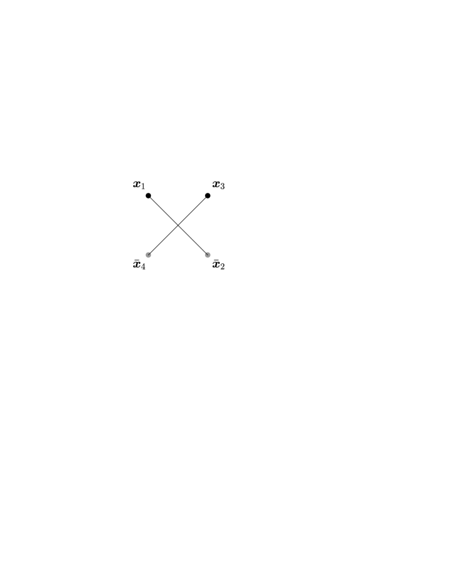
(a)

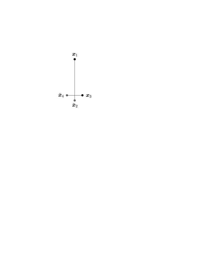
(b)

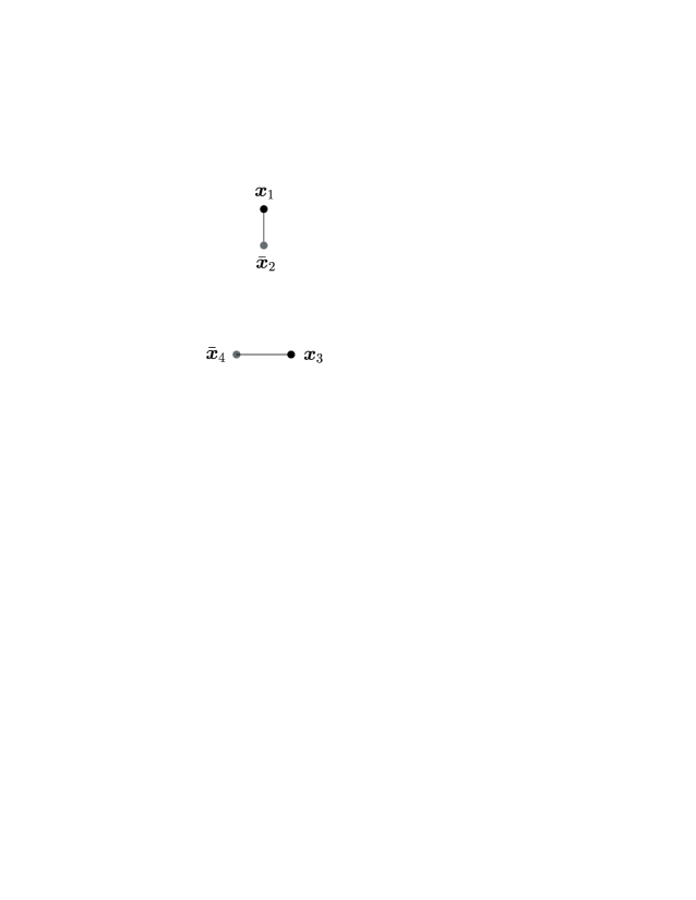
(c)

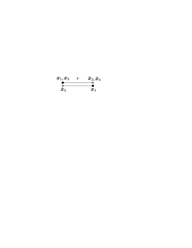
(d)

Figure 3: (a), (b) and (c) correspond to special configurations of the quadrupole for which $r_{13}=r_{14}$ and $r_{23}=r_{24}$. In (a) $r_{12}=r_{34}$ and all $r_{ij}$ of the same order, in (b) $r_{34}\ll r_{12}\sim r_{14}$ and in (c) $r_{12}\sim r_{34}\ll r_{14}$. The average values of $\hat{Q}$ and $\hat{S}_{6}$ depend only on the distances depicted by straight lines. Figure (d) corresponds to the line configuration for the operator $\hat{S}_{6}$.

Now let us proceed to our second example and consider the operator

$$\hat{Q}_{\bm{x}_{1}\bm{x}_{2}\bm{x}_{3}\bm{x}_{4}}\hat{S}_{\bm{x}_{4}\bm{x}_{3}}=\frac{1}{N_{c}}\,{\rm tr}({V}^{\dagger}_{\bm{x}_{1}}{V}_{\bm{x}_{2}}{V}^{\dagger}_{\bm{x}_{3}}{V}_{\bm{x}_{4}})\,\frac{1}{N_{c}}\,{\rm tr}({V}^{\dagger}_{\bm{x}_{4}}{V}_{\bm{x}_{3}}).$$ (4.37)

The choice is of direct phenomenological interest, since the operator above is the most complicated quantity appearing in the calculation of di–hadron production in proton–nucleus collisions JalilianMarian:2004da ; Nikolaev:2005dd ; Baier:2005dv ; Marquet:2007vb . Considering the same configuration as before, that is, taking $r_{13}=r_{14}$ and $r_{23}=r_{24}$, we see that the evolution couples the operator in Eq. (4.37) to $\hat{S}_{\bm{x}_{1}\bm{x}_{2}}\hat{S}_{\bm{x}_{1}\bm{x}_{2}}\hat{S}_{\bm{x}_{2}\bm{x}_{1}}$. After a straightforward calculation, similar to the one leading at Eq. (4.36), we arrive at

$$\langle\hat{Q}_{\bm{x}_{1}\bm{x}_{2}\bm{x}_{3}\bm{x}_{4}}\hat{S}_{\bm{x}_{4}\bm{x}_{3}}\rangle_{Y}=\langle\hat{S}_{\bm{x}_{1}\bm{x}_{2}}\hat{S}_{\bm{x}_{3}\bm{x}_{4}}\hat{S}_{\bm{x}_{4}\bm{x}_{3}}\rangle_{Y}=\frac{N_{c}^{2}-1}{N_{c}^{2}}\,\langle\hat{S}_{\bm{x}_{1}\bm{x}_{2}}\rangle_{Y}\langle\hat{S}_{\bm{x}_{3}\bm{x}_{4}}\rangle_{Y}^{\textstyle\frac{2N_{c}^{2}}{N_{c}^{2}-1}}+\frac{1}{N_{c}^{2}}\,\langle\hat{S}_{\bm{x}_{1}\bm{x}_{2}}\rangle_{Y}.$$ (4.38)

(Once again, we have assumed this equation to hold already in the initial condition at $Y_{0}$, which is in particular true within the MV model, as one can check.) It is interesting that for this configuration, and similar to Eq. (4.36), the result depends only on $r_{12}$ and $r_{34}$, but not on $r_{14}$ and $r_{23}$. Also, by keeping $N_{c}$ finite, we notice that the last term in the r.h.s. (the single dipole $S$–matrix) dominates deeply at saturation. This is in agreement with our earlier discussion in 3.4, since the linear combination

$$\hat{Q}_{\bm{x}_{1}\bm{x}_{2}\bm{x}_{3}\bm{x}_{4}}\hat{S}_{\bm{x}_{4}\bm{x}_{3}}-\frac{1}{N_{c}^{2}}\,\hat{S}_{\bm{x}_{1}\bm{x}_{2}}$$ (4.39)

is a special case of the operator in Eq. (3.37) for this particular configuration. In fact, the operator that appears in the di–hadron cross section is the combination

$$\hat{S}_{6\,\bm{x}_{1}\bm{x}_{2}\bm{x}_{3}\bm{x}_{4}}=\frac{N_{c}^{2}}{N_{c}^{2}-1}\,\hat{Q}_{\bm{x}_{1}\bm{x}_{2}\bm{x}_{3}\bm{x}_{4}}\hat{S}_{\bm{x}_{4}\bm{x}_{3}}-\frac{1}{N_{c}^{2}-1}\,\hat{S}_{\bm{x}_{1}\bm{x}_{2}},$$ (4.40)

which is also the quantity studied numerically in Dumitru:2011vk . Using the previous results one finds that, for our special configuration, the expectation value of $\hat{S}_{6}$ is given by the relatively simple expression

$$\langle\hat{S}_{6\,\bm{x}_{1}\bm{x}_{2}\bm{x}_{3}\bm{x}_{4}}\rangle_{Y}=\langle\hat{S}_{\bm{x}_{1}\bm{x}_{2}}\rangle_{Y}\Big{[}\langle\hat{S}_{\bm{x}_{3}\bm{x}_{4}}\rangle_{Y}\Big{]}^{\textstyle\frac{2N_{c}^{2}}{N_{c}^{2}-1}}.$$ (4.41)

It is amusing to note that for this particular configuration and for large $N_{c}$, the 4–point function relevant for di–hadron production factorizes as $\langle\hat{S}_{6\,\bm{x}_{1}\bm{x}_{2}\bm{x}_{3}\bm{x}_{4}}\rangle_{Y}=\langle\hat{S}_{\bm{x}_{1}\bm{x}_{2}}\rangle_{Y}\hat{S}_{\bm{x}_{3}\bm{x}_{4}}\rangle_{Y}^{2}$. This is precisely the factorization formula used (for a generic configuration) in the phenomenological study in Albacete:2010pg — at that time, by lack of a better formula. Such a factorization however has no deep justification and is merely a property of the configuration at hand. As our next example will show, this ‘factorization’ can badly fail for other, equally simple, configurations.

Specifically, let us consider the expectation value of the operator (4.37) for the ‘line’ configuration studied in Dumitru:2011vk ; Iancu:2011ns and shown in Fig. 3.d. Note that the two quarks of the quadrupole and the antiquark of the dipole are put in a same point ($\bm{x}_{1}=\bm{x}_{3}$), and similarly for the two antiquarks of the quadrupole and the quark in the dipole ($\bm{x}_{2}=\bm{x}_{4}$). Thus, only one non–trivial distance $r\equiv r_{12}=r_{23}=r_{34}=r_{14}$ characterizes the configuration. Then one can easily check that the evolution of $\hat{Q}_{\bm{x}_{1}\bm{x}_{2}\bm{x}_{1}\bm{x}_{2}}\hat{S}_{\bm{x}_{2}\bm{x}_{1}}$ couples again to $\hat{S}_{\bm{x}_{1}\bm{x}_{2}}\hat{S}_{\bm{x}_{1}\bm{x}_{2}}\hat{S}_{\bm{x}_{2}\bm{x}_{1}}$, leading to a $2\mspace{-2.0mu}\times\mspace{-2.0mu}2$ inhomogeneous system of equations. Expressing $\gamma_{Y}(r)$ in terms of the dipole $\langle\hat{S}(r)\rangle_{Y}$ and using an obvious shorthand notation we have

$$\frac{\partial\langle\hat{Q}\hat{S}\rangle_{Y}}{\partial\ln\langle\hat{S}\rangle_{Y}}=\frac{3N_{c}^{2}-1}{N_{c}^{2}-1}\,\langle\hat{Q}\hat{S}\rangle_{Y}+\frac{2N_{c}^{2}}{N_{c}^{2}-1}\,\langle\hat{S}^{3}\rangle_{Y}-\frac{4}{N_{c}^{2}-1}\,\langle\hat{S}\rangle_{Y},$$ (4.42)

$$\frac{\partial\langle\hat{S}^{3}\rangle_{Y}}{\partial\ln\langle\hat{S}\rangle_{Y}}=\frac{2}{N_{c}^{2}-1}\,\langle\hat{Q}\hat{S}\rangle_{Y}+\frac{3N_{c}^{2}-1}{N_{c}^{2}-1}\,\langle\hat{S}^{3}\rangle_{Y}-\frac{4}{N_{c}^{2}-1}\,\langle\hat{S}\rangle_{Y}.$$ (4.43)

The solution to this system is straightforward to obtain; so long as $\langle\hat{Q}\hat{S}\rangle_{Y}$ is concerned, one finds

$$\langle\hat{Q}\hat{S}\rangle_{Y}=\frac{(N_{c}+2)(N_{c}-1)}{2N_{c}}\,\langle\hat{S}\rangle_{Y}^{\textstyle{\frac{3N_{c}-1}{N_{c}-1}}}-\frac{(N_{c}+1)(N_{c}-2)}{2N_{c}}\,\langle\hat{S}\rangle_{Y}^{\textstyle{\frac{3N_{c}+1}{N_{c}+1}}},$$ (4.44)

where we assumed that the above is already valid at $Y_{0}$, as is the case in the MV model. Using this result together with Eq. (4.40), it is straightforward to evaluate $\langle\hat{S}_{6}\rangle_{Y}$ for this particular configuration and compare with the numerical results in Ref. Dumitru:2011vk . We shall find it rewarding to plot $\langle\hat{S}_{6}\rangle_{Y}$ in two different ways; first as a function of $rQ_{s}$ and then as a function of $1-\langle\hat{S}\rangle_{Y}$. To be in accordance with Dumitru:2011vk , the saturation momentum is defined by the condition $\langle\hat{S}\rangle_{Y}=1/\sqrt{e}$ for $rQ_{s}=\sqrt{2}$.

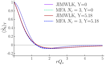
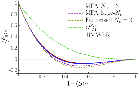
Figure 4: The expectation value of $\hat{S}_{6}$, as defined in Eq. (4.40), for the ‘line’ configuration. Left: as a function of the scaling variable $rQ_{s}$. Continuous magenta: JIMWLK at Y=0. Dashed cyan: MFA for $N_{c}$=3 at Y=0. Continuous red: JIMWLK at Y=5.18. Dashed blue: MFA for $N_{c}$=3 at Y=5.18. Right: as a function of $1\!-\!\langle\hat{S}\rangle_{Y}$. Continuous red: JIMWLK at six different values of rapidity Y=0, 1.04, 2.07, 3.11, 4.14 and 5.18. Continuous blue: complete result in the MFA for $N_{c}=3$. Dashed magenta: large–$N_{c}$ result in the MFA. Dotted gold: assuming factorization for the expectation value of $\hat{Q}\hat{S}$ and using the MFA for $N_{c}=3$ for the expectation value of the quadrupole $\hat{Q}$. Dotted dashed green: for illustrative purposes we also show $\langle\hat{S}\rangle_{Y}^{3}$. JIMWLK curves are constructed from the numerical solution given in Dumitru:2011vk . MFA curves are analytical expressions in terms of $\langle\hat{S}\rangle$, which is again provided by the numerical solution in Dumitru:2011vk for the purposes of the left figure.

We show this comparison in Fig. 4, where for some of the curves we have used the numerical data of Dumitru:2011vk . On the left we show the correlator of interest as a function of $rQ_{s}$ and for two values of the rapidity: $Y=0$, which is where one starts the evolution (with initial conditions of the MV type), and $Y=5.18$, which is large enough for the effects of the evolution to be fully developed. The curves denoted as ‘MFA’ represent our present results, cf. Eq. (4.44) and (4.40), whereas the ‘JIMWLK’ curves follow from the numerical solution to the JIMWLK equation. For $Y=0$, the two types of curves overlap with each by construction, as they both reduce to the respective prediction of the MV model. What is remarkable though, is that a very good agreement between the numerical solution and the MFA persists for $Y=5.18$. In the limiting regimes of weak and respectively strong scattering, the respectives curves are practically indistinguishable. In the transition region around $rQ_{s}\sim 1$, the agreement is not that perfect anymore, but the two curves are still very close to each other, confirming that the MFA is also an excellent global approximation.

From Fig. 4 (left) we also notice that the shape of the curve changes as we evolve from $Y=0$ to higher values of rapidity ($Y=5.18$ in the figure). However, this change is mostly attributed to the evolution of $\langle\hat{S}\rangle_{Y}$ as a function of $rQ_{s}$ as the rapidity grows. Indeed, in the right panel of Fig. 4 we show the correlator of interest as a function of $1-\langle\hat{S}\rangle_{Y}$. One can see that the curves obtained from the numerical solution to JIMWLK for various values of $Y$ form a very thin “band” whose borderline on the “lower” side is the MFA. This “band” is practically a line perfectly overlapping with the MFA when the scattering is either weak or strong, and becomes just a bit wider in the transition region. Thus, as we evolve in rapidity, the shape of the curve is barely changing. In fact, if one expands out the plot in order to better disentangle the various steps in the evolution, one can see that the high–$Y$ curve stabilizes very close to the $Y=0$ curve after just a few units in rapidity.

Still in the right plot we also show two different approximations for $\langle\hat{S}_{6}\rangle_{Y}$, the one is the large-$N_{c}$ result, while the other consists of factorizing $\langle\hat{Q}\hat{S}\rangle_{Y}$ into $\langle\hat{Q}\rangle_{Y}\langle\hat{S}\rangle_{Y}$, as it would be justified at large $N_{c}$, but then using the finite–$N_{c}$ Gaussian approximation for $\langle\hat{Q}\rangle_{Y}$. This latter approximation takes into account some $1/N_{c}^{2}$ corrections, but not in a systematic way, and was used in Dumitru:2011vk since the (MV–like) expression (4.44) was not available at the time. Comparing with the numerical findings in Dumitru:2011vk , we already saw that the complete result Eq. (4.44) at finite–$N_{c}$ is the one which shows the best agreement. Even though it is not very significant, we note that the large–$N_{c}$ expression is the next one closer to the numerical data, perhaps because it is at least a systematic approximation. For illustrative purposes we also show $\langle\hat{S}\rangle_{Y}^{3}$, which is based neither on a large–$N_{c}$ approximation nor on a mean field one, but simply corresponds to a ‘naive’ counting of Wilson lines. It fails badly even in the BFKL regime and clearly it has no chance to describe properly the correlator of interest.

References

- (1) E. Braidot, “Two-particle azimuthal correlations at forward rapidity in STAR,” 1102.0931.
- (2) C. Marquet, “Forward inclusive dijet production and azimuthal correlations in pA collisions,” Nucl. Phys. A796 (2007) 41–60, 0708.0231.
- (3) J. Jalilian-Marian and Y. V. Kovchegov, “Inclusive two-gluon and valence quark-gluon production in DIS and p A,” Phys. Rev. D70 (2004) 114017, hep-ph/0405266.
- (4) R. Baier, A. Kovner, M. Nardi, and U. A. Wiedemann, “Particle correlations in saturated QCD matter,” Phys. Rev. D72 (2005) 094013, hep-ph/0506126.
- (5) N. N. Nikolaev, W. Schafer, B. G. Zakharov, and V. R. Zoller, “Nonlinear k(T)-factorization for quark-gluon dijet production off nuclei,” Phys. Rev. D72 (2005) 034033, hep-ph/0504057.
- (6) J. L. Albacete and C. Marquet, “Azimuthal correlations of forward di-hadrons in d+Au collisions at RHIC in the Color Glass Condensate,” Phys. Rev. Lett. 105 (2010) 162301, 1005.4065.
- (7) A. Stasto, B.-W. Xiao, and F. Yuan, “Back-to-Back Correlations of Di-hadrons in dAu Collisions at RHIC,” 1109.1817.
- (8) F. Dominguez, C. Marquet, B.-W. Xiao, and F. Yuan, “Universality of Unintegrated Gluon Distributions at small x,” Phys. Rev. D83 (2011) 105005, 1101.0715.
- (9) A. Dumitru and J. Jalilian-Marian, “Forward dijets in high-energy collisions: evolution of QCD n-point functions beyond the dipole approximation,” Phys. Rev. D82 (2010) 074023, 1008.0480.
- (10) F. Dominguez, A. H. Mueller, S. Munier, and B.-W. Xiao, “On the small-x evolution of the color quadrupole and the Weizsácker-Williams gluon distribution,” Phys. Lett. B705 (2011) 106–111, 1108.1752.
- (11) A. Dumitru, J. Jalilian-Marian, T. Lappi, B. Schenke, and R. Venugopalan, “Renormalization group evolution of multi-gluon correlators in high energy QCD,” Phys. Lett. B706 (2011) 219–224, 1108.4764.
- (12) E. Iancu and D. N. Triantafyllopoulos, “Higher-point correlations from the JIMWLK evolution,” JHEP 11 (2011) 105, 1109.0302.
- (13) J. Jalilian-Marian, A. Kovner, A. Leonidov, and H. Weigert, “The BFKL equation from the Wilson renormalization group,” Nucl. Phys. B504 (1997) 415–431, hep-ph/9701284.
- (14) J. Jalilian-Marian, A. Kovner, A. Leonidov, and H. Weigert, “The Wilson renormalization group for low x physics: Towards the high density regime,” Phys. Rev. D59 (1999) 014014, hep-ph/9706377.
- (15) J. Jalilian-Marian, A. Kovner, and H. Weigert, “The Wilson renormalization group for low x physics: Gluon evolution at finite parton density,” Phys. Rev. D59 (1999) 014015, hep-ph/9709432.
- (16) A. Kovner, J. G. Milhano, and H. Weigert, “Relating different approaches to nonlinear QCD evolution at finite gluon density,” Phys. Rev. D62 (2000) 114005, hep-ph/0004014.
- (17) H. Weigert, “Unitarity at small Bjorken x,” Nucl. Phys. A703 (2002) 823–860, hep-ph/0004044.
- (18) E. Iancu, A. Leonidov, and L. D. McLerran, “Nonlinear gluon evolution in the color glass condensate. I,” Nucl. Phys. A692 (2001) 583–645, hep-ph/0011241.
- (19) E. Iancu, A. Leonidov, and L. D. McLerran, “The renormalization group equation for the color glass condensate,” Phys. Lett. B510 (2001) 133–144, hep-ph/0102009.
- (20) E. Ferreiro, E. Iancu, A. Leonidov, and L. McLerran, “Nonlinear gluon evolution in the color glass condensate. II,” Nucl. Phys. A703 (2002) 489–538, hep-ph/0109115.
- (21) I. Balitsky, “Operator expansion for high-energy scattering,” Nucl. Phys. B463 (1996) 99–160, hep-ph/9509348.
- (22) A. Dumitru, E. Iancu, L. Portugal, G. Soyez, and D. N. Triantafyllopoulos, “Pomeron loop and running coupling effects in high energy QCD evolution,” JHEP 08 (2007) 062, 0706.2540.
- (23) E. Iancu and D. N. Triantafyllopoulos, “A Langevin equation for high energy evolution with pomeron loops,” Nucl. Phys. A756 (2005) 419–467, hep-ph/0411405.
- (24) A. H. Mueller, A. I. Shoshi, and S. M. H. Wong, “Extension of the JIMWLK equation in the low gluon density region,” Nucl. Phys. B715 (2005) 440–460, hep-ph/0501088.
- (25) E. Iancu and D. N. Triantafyllopoulos, “Non-linear QCD evolution with improved triple-pomeron vertices,” Phys. Lett. B610 (2005) 253–261, hep-ph/0501193.
- (26) A. Kovner and M. Lublinsky, “In pursuit of pomeron loops: The JIMWLK equation and the Wess-Zumino term,” Phys. Rev. D71 (2005) 085004, hep-ph/0501198.
- (27) E. Iancu, A. H. Mueller, and S. Munier, “Universal behavior of QCD amplitudes at high energy from general tools of statistical physics,” Phys. Lett. B606 (2005) 342–350, hep-ph/0410018.
- (28) J.-P. Blaizot, E. Iancu, and H. Weigert, “Non linear gluon evolution in path-integral form,” Nucl. Phys. A713 (2003) 441–469, hep-ph/0206279.
- (29) L. D. McLerran and R. Venugopalan, “Computing quark and gluon distribution functions for very large nuclei,” Phys. Rev. D49 (1994) 2233–2241, hep-ph/9309289.
- (30) L. D. McLerran and R. Venugopalan, “Gluon distribution functions for very large nuclei at small transverse momentum,” Phys. Rev. D49 (1994) 3352–3355, hep-ph/9311205.
- (31) J. P. Blaizot, F. Gelis, and R. Venugopalan, “High energy p A collisions in the color glass condensate approach. II: Quark production,” Nucl. Phys. A743 (2004) 57–91, hep-ph/0402257.
- (32) A. Kovner and U. A. Wiedemann, “Eikonal evolution and gluon radiation,” Phys. Rev. D64 (2001) 114002, hep-ph/0106240.
- (33) J. Kuokkanen, K. Rummukainen, and H. Weigert, “HERA-data in the light of small x evolution with state of the art NLO input,” 1108.1867.
- (34) B. Muller and A. Schafer, “Transverse energy density fluctuations in the Color Glass Condensate Model,” 1111.3347.
- (35) C. Marquet and H. Weigert, “New observables to test the Color Glass Condensate beyond the large– limit,” Nucl. Phys. A843 (2010) 68–97, 1003.0813.
- (36) E. Iancu, A. Leonidov, and L. McLerran, “The colour glass condensate: An introduction,” hep-ph/0202270.
- (37) Y. V. Kovchegov, J. Kuokkanen, K. Rummukainen, and H. Weigert, “Subleading– corrections in non-linear small-x evolution,” Nucl. Phys. A823 (2009) 47–82, 0812.3238.
- (38) E. Iancu, K. Itakura, and L. McLerran, “A Gaussian effective theory for gluon saturation,” Nucl. Phys. A724 (2003) 181–222, hep-ph/0212123.
- (39) E. Iancu and L. D. McLerran, “Saturation and universality in QCD at small x,” Phys. Lett. B510 (2001) 145–154, hep-ph/0103032.
- (40) E. Iancu and R. Venugopalan, “The color glass condensate and high energy scattering in QCD,” hep-ph/0303204.
- (41) Y. V. Kovchegov, “Small-x F2 structure function of a nucleus including multiple pomeron exchanges,” Phys. Rev. D60 (1999) 034008, hep-ph/9901281.
- (42) Y. Hatta, E. Iancu, K. Itakura, and L. McLerran, “Odderon in the color glass condensate,” Nucl. Phys. A760 (2005) 172–207, hep-ph/0501171.
- (43) D. N. Triantafyllopoulos, “Pomeron loops in high energy QCD,” Acta Phys. Polon. B36 (2005) 3593–3664, hep-ph/0511226.
- (44) A. Kovner and M. Lublinsky, “Remarks on high energy evolution,” JHEP 03 (2005) 001, hep-ph/0502071.
- (45) A. Kovner and M. Lublinsky, “From target to projectile and back again: selfduality of high energy evolution,” Phys. Rev. Lett. 94 (2005) 181603, hep-ph/0502119.
- (46) L. Lipatov, “Reggeization of the Vector Meson and the Vacuum Singularity in Nonabelian Gauge Theories,” Sov.J.Nucl.Phys. 23 (1976) 338–345.
- (47) E. Kuraev, L. Lipatov, and V. S. Fadin, “The Pomeranchuk Singularity in Nonabelian Gauge Theories,” Sov.Phys.JETP 45 (1977) 199–204.
- (48) I. Balitsky and L. Lipatov, “The Pomeranchuk Singularity in Quantum Chromodynamics,” Sov.J.Nucl.Phys. 28 (1978) 822–829.
- (49) E. Iancu, K. Itakura, and L. McLerran, “Geometric scaling above the saturation scale,” Nucl. Phys. A708 (2002) 327–352, hep-ph/0203137.
- (50) A. H. Mueller and D. N. Triantafyllopoulos, “The energy dependence of the saturation momentum,” Nucl. Phys. B640 (2002) 331–350, hep-ph/0205167.
- (51) S. Munier and R. B. Peschanski, “Geometric scaling as traveling waves,” Phys. Rev. Lett. 91 (2003) 232001, hep-ph/0309177.
- (52) J. Bartels, “High-Energy Behavior in a Nonabelian Gauge Theory. 2. First Corrections to Beyond the Leading LNS Approximation,” Nucl.Phys. B175 (1980) 365.
- (53) J. Kwiecinski and M. Praszalowicz, “Three Gluon Integral Equation and Odd c Singlet Regge Singularities in QCD,” Phys.Lett. B94 (1980) 413.
- (54) T. Jaroszewicz, “Infrared Divergences and Regge Behavior in QCD,” Acta Phys.Polon. B11 (1980) 965.
- (55) S. Jeon and R. Venugopalan, “A classical odderon in QCD at high energies,” Phys. Rev. D71 (2005) 125003, hep-ph/0503219.
- (56) E. Levin and K. Tuchin, “Solution to the evolution equation for high parton density QCD,” Nucl. Phys. B573 (2000) 833–852, hep-ph/9908317.
- (57) E. Iancu and A. H. Mueller, “Rare fluctuations and the high-energy limit of the S- matrix in QCD,” Nucl. Phys. A730 (2004) 494–513, hep-ph/0309276.
- (58) A. H. Mueller, “Gluon distributions and color charge correlations in a saturated light-cone wavefunction,” Nucl. Phys. B643 (2002) 501–513, hep-ph/0206216.
- (59) K. Rummukainen and H. Weigert, “Universal features of JIMWLK and BK evolution at small x,” Nucl. Phys. A739 (2004) 183–226, hep-ph/0309306.
- (60) T. Lappi, “Gluon spectrum in the glasma from JIMWLK evolution,” 1105.5511.
- (61) K. J. Golec-Biernat and M. Wusthoff, “Saturation effects in deep inelastic scattering at low and its implications on diffraction,” Phys. Rev. D59 (1998) 014017, hep-ph/9807513.
- (62) K. J. Golec-Biernat and M. Wusthoff, “Saturation in diffractive deep inelastic scattering,” Phys. Rev. D60 (1999) 114023, hep-ph/9903358.
- (63) D. Binosi and L. Theussl, “JaxoDraw: A graphical user interface for drawing Feynman diagrams,” Comput. Phys. Commun. 161 (2004) 76–86, hep-ph/0309015.
- (64) D. Binosi, J. Collins, C. Kaufhold, and L. Theussl, “JaxoDraw: A graphical user interface for drawing Feynman diagrams. Version 2.0 release notes,” Comput. Phys. Commun. 180 (2009) 1709–1715, 0811.4113.